Edelstein-Keshet L. Mathematical Models in Biology
Подождите немного. Документ загружается.

76
Discrete Processes
in
Biology
We
observe
that when
N < K the
reproductive rate
A > 1,
whereas when
N > K,
A
< 1
(see
problem
3).
This property
is
shared with equation (11)
of
Chapter
2
where
K = 1. K is
said
to be the
carrying
capacity
of the
environment
for the
popu-
lation.
In the
next chapter
we
shall
see
examples
of
similar density-dependent rela-
tionships
within
the
framework
of
continuous populations.
3. Yet a
third
model,
proposed
by
Hassell (1975),
is
given
by the
equation
for
A, a, b
positive
constants. Analysis
of
this equation
is
left
as a
pr lem
for the
reader.
One
generally observes with models such
as
1,2,
and 3
(and with other dis-
crete equations such
as the
prototype given
in
Chapter
2)
that
the
dynamical behav-
ior
depends
in a
sensitive
way on
parameter settings. Typically such equations have
stable cycles
of
arbitrary periods
as
well
as
chaotic behavior. Each model thus
de-
scribes
a
highly complex range
of
dynamic behavior
if
parameter values
are
pushed
to
high
values.
For
example,
equation (13)
has the
behavioral
regimes
mapped
out
on
the
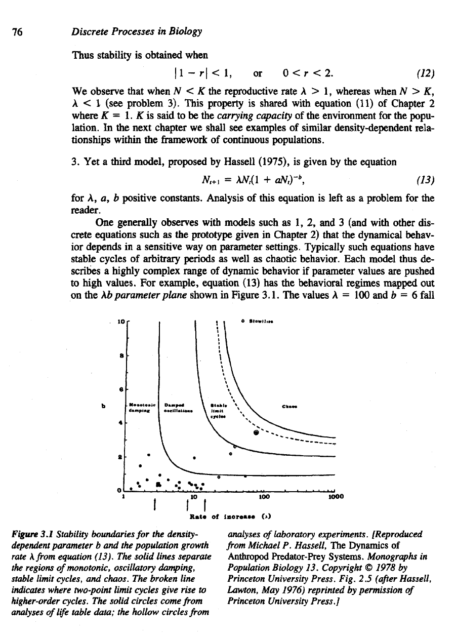
Xb
parameter plane shown
in
Figure 3.1.
The
values
A = 100 and b = 6
fall
Figure
3.1
Stability
boundaries
for the
density-
dependent
parameter
b and the
population growth
rate
\from
equation (13).
The
solid lines separate
the
regions ofmonotonic, oscillatory damping,
stable
limit cycles,
and
chaos.
The
broken line
indicates
where two-point limit cycles give rise
to
higher-order
cycles.
The
solid circles come
from
analyses
of
life
table data;
the
hollow circles
from
analyses
of
laboratory
experiments.
[Reproduced
from
Michael
P.
Hassell,
The
Dynamics
of
Anthropod
Predator-Prey
Systems.
Monographs
in
Population
Biology
13.
Copyright
©
1978
by
Princeton
University
Press.
Fig.
2.5
(after
Hassell,
Lawton,
May
1976) reprinted
by
permission
of
Princeton
University
Press.]
Thus
stability
is
obtained
when
Applications
of
Nonlinear
Difference
Equations
to
Population
Biology
77
in
the
chaotic
domain,
so
that populations
fluctuate
wildly.
The
values
A = 100 and
b =
0.5, correspond
to a
stable steady state,
so
that
a
perturbed population under-
goes monotonic damping back
to its
steady-state level.
For a
given
single-species
population, density
fluctuations may or may not be
described well
by a
model such
as
equation (13),
If so,
parameters
such
as b and A
can be
estimated
by
following
the
observed levels
of the
population over successive
generations. Such observations
are
called
life
table
data. Studies
of
this sort have
been carried
out
under
a
variety
of
conditions, both
in the field and in
laboratory set-
tings (see Hassell
et
al., 1976). Typical species observed
in the field
have included
insects such
as the
moth
Zeiraphera
diniana
and the
parasitoid
fly
Cyzenis
albicans.
Laboratory data
on
beetles
and on the
blowfly
Lucilia
cuprina
(Nicholson, 1954)
have also been
collected.
Pooling results
of
many
observations
in the
literature
and in
their
own
experi-
ments,
Hassell
et al.
(1976)
plotted
the
parameter values
b and A of
some
two
dozen
species
on the b\
parameter plane.
In all but two of
these cases,
the
values
of b and
A
obtained were well within
the
region
of
stability; that
is,
they
reflected either
monotonic
or
oscillatory
return
to the
steady states.
Hassell
et al.
(1976)
found
two
examples
of
unstable populations.
The
only
one
occurring
in a
natural system
was
that
of the
Colorado
potato beetle (shown
as a
circled
dot in
Figure 3.1), which
is
known
to fluctuate
periodically
in
certain situa-
tions.
A
single
laboratory population, that
of the
blowfly
(Nicholson,
1954),
was
found
to
have
(A, b)
values corresponding
to the
chaotic regime
in
Figure 3.1. Some
controversy surrounds
the
acceptance
of
this single example
as a
true case
of
chaotic
population dynamics.
From
their particular
set of
examples, Hassel
et al.
(1976) concluded that com-
plex behavioral
regimes
typical
of
discrete
difference
equations
are not
frequently
observed
in
reality.
Of
course,
to
place this deduction
in its
proper context,
we
should
remember that only
a relatively
small sample
of
species
has
been
sufficiently
well studied
to be represented, and
that Figure
3.1
describes
the fit to one
particular
model,
chosen
somewhat arbitrarily
from
many
equally plausible ones.
One of the
contributions
of
mathematical modeling
and
analysis
to the
study
of
population behavior
has
been
in
bringing
forward
questions that might otherwise
have
been
of
lesser
interest. Comparison between observations
and
model predic-
tions
indicate that many dynamical behavior patterns, which
are
theoretically possi-
ble,
are not
observed
in
nature.
We are
thereby
led to
inquire which
effects
in
natu-
ral
systems have stabilizing
influences
on
populations that might otherwise behave
chaotically.
Hassell
et al.
(1976) comment
on
some
of the key
elements
of
studies based
on
data
collected
in the field
versus those collected under controlled laboratory condi-
tions.
In the
former,
the
survival
of a
population
may
depend
on
multiple factors
in-
cluding
predation, parasitism, competition,
and
environmental conditions (see Sec-
tions
3.2–3.4).
Thus
a
description
of the
population
by a
single-species model
is, at
best,
a
crude approximation.
Laboratory experiments
on the
other hand,
can
provide conditions
in
which
a
population
is
truly
isolated
from
other species.
In
this sense, such data
is
more suit-
able
for
interpretation
by
single-species models. However,
the
influence
of a
some-
what
artificial setting
may
result
in
effects
(such
as
competitio
close
78
Discrete Processes
in
Biology
confinement) that
are not
significant
in the
natural setting. Thus, data
for
laboratory
studies such
as
those
of
Nicholson's blowflies,
in
which erratic chaotic behavior
is
observed,
may
reflect
not a
realistic
trend
but
rather
an
artifact observed only
in
the
laboratory.
3.2
TWO-SPECIES
INTERACTIONS:
HOST-PARASITOID SYSTEMS
Discrete difference-equation models apply most readily
to
groups
such
as
insect pop-
ulations where there
is a
rather natural division
of
time into discrete generations.
In
this
section
we
examine
a
particular two-species model that
has
received consider-
able attention
from
experimental
and
theoretical population biologists, that
of the
host-parasitoid
system.
Found almost entirely
in the
world
of
insects, such two-species systems have
several distinguishing features. Typical
of
insect species, both species have
a
num-
ber of
life-cycle stages that include eggs, larvae, pupae
and
adults.
One of the
spe-
cies,
called
fas
parasitoid, exploits
the
second
in the
following way:
An
adult female
parasitoid searches
for a
host
on
which
to
oviposit
(deposit
its
eggs).
In
some cases
eggs
are
attached
to the
outer surface
of the
host during
its
larval
or
pupal stage.
In
other
cases
the
eggs
are
injected into
the
host's
flesh. The
larval parasitoids develop
and
grow
at the
expense
of
their host, consuming
it and
eventually killing
it
before
they
pupate.
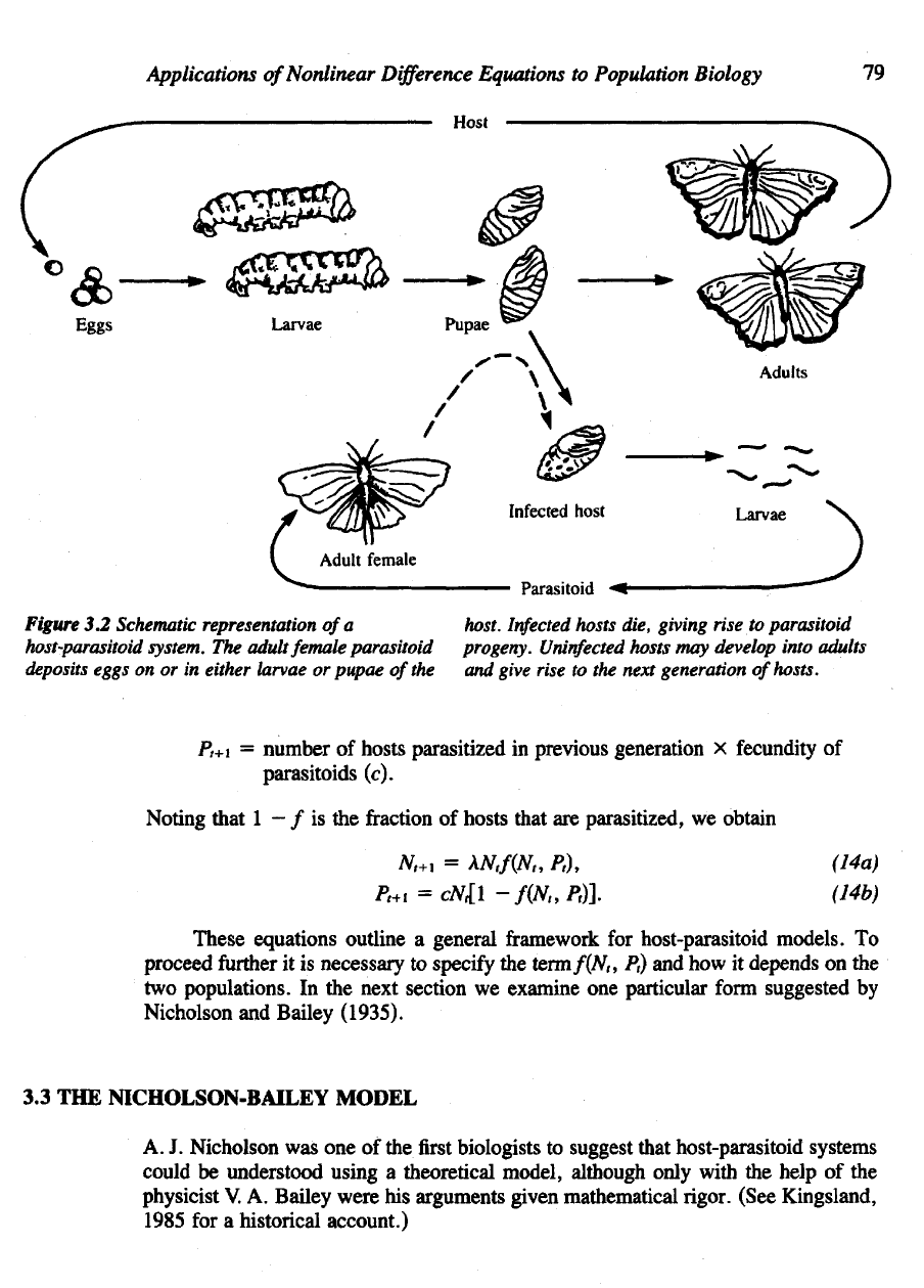
The
life
cycles
of the two
species, shown
in
Figure 3.2,
are
thus closely
intertwined.
A
simple model
for
this system
has the
following common
set of
assumptions:
1.
Hosts
that
have been parasitized will give rise
to the
next generation
of
parasitoids.
2.
Hosts that have
not
been parasitized will give rise
to
their
own
progeny.
3. The
fraction
of
hosts that
are
parasitized depends
on the
rate
of
encounter
of
the two
species;
in
general, this fraction
may
depend
on the
densities
of one or
both
species.
While other
effects
causing mortality abound
in any
natural system,
it is in-
structive
to
consider only this minimal
set of
interactions
first and
examine their con-
sequences.
We
therefore
define
the
following:
N
t
=
density
of
host species
in
generation
t,
P
t
=
density
of
parasitoid
in
generation
t,
/ =
f(N,,
P
t
)
=
fraction
of
hosts
not
parasitized,
A
=
host reproductive
rate,
c =
average number
of
viable eggs laid
by a
parasitoid
on a
single host.
Then
our
three assumptions lead
to:
N
t
+i
=
number
of
hosts
in
previous generation
X
fraction
not
parasitized
x
reproductive rate (A),
Applications
of
Nonlinear
Difference
Equations
to
Population
Biology
79
Figure
3.2
Schematic
representation
of
a
host.
Infected
hosts
die,
giving
rise
to
parasitoid
host-parasitoid
system.
The
adult
female
parasitoid progeny.
Uninfected
hosts
may
develop
into
adults
deposits
eggs
on or in
either
larvae
or
pupae
of
the and
give
rise
to the
next
generation
of
hosts.
P
t
+i
=
number
of
hosts parasitized
in
previous generation
x
fecundity
of
parasitoids (c).
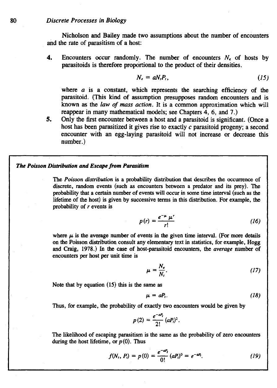
Noting that
1
—
/ is the
fraction
of
hosts that
are
parasitized,
we
obtain
3.3 THE
NICHOLSON-BAILEY MODEL
A.
J.
Nicholson
was one of the first
biologists
to
suggest that host-parasitoid systems
could
be
understood using
a
theoretical
model, although only with
the
help
of the
physicist
V. A.
Bailey were
his
arguments given mathematical
rigor.
(See Kingsland,
1985
for a
historical account.)
These equations outline
a
general
framework
for
host-parasitoid models.
To
proceed
further
it is
necessary
to
specify
the
term/(M,
Pt)
and how it
depends
on the
two
populations.
In the
next section
we
examine
one
particular
form
suggested
by
Nicholson
and
Bailey (1935).
80
Discrete Processes
in
Biology
Nicholson
and
Bailey made
two
assumptions about
the
number
of
encounters
and
the
rate
of
parasitism
of a
host:
4.
Encounters occur randomly.
The
number
of
encounters
N
e
of
hosts
by
parasitoids
is
therefore proportional
to the
product
of
their densities.
The
Poisson Distribution
and
Escape from Parasitism
The
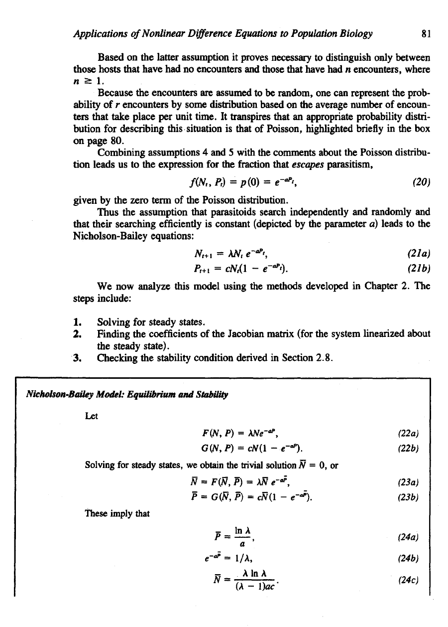
Poisson distribution
is a
probability distribution that
describes
the
occurrence
of
discrete,
random events (such
as
encounters between
a
predator
and its
prey).
The
probability that
a
certain number
of
events will occur
in
some time interval (such
as the
lifetime
of the
host)
is
given
by
successive
terms
in
this distribution.
For
example,
the
probability
of r
events
is
where
a is a
constant, which represents
the
searching
efficiency
of the
parasitoid. (This kind
of
assumption presupposes random encounters
and is
known
as the law of
mass action.
It is a
common approximation which will
reappear
in
many mathematical models;
see
Chapters
4, 6, and 7.)
5.
Only
the first
encounter between
a
host
and a
parasitoid
is
significant.
(Once
a
host
has
been parasitized
it
gives
rise to
exactly
c
parasitoid progeny;
a
second
encounter with
an
egg-laying parasitoid
will
not
increase
or
decrease this
number.)
where
/x, is the
average number
of
events
in the
given time interval. (For more details
on
the
Poisson distribution consult
any
elementary text
in
statistics,
for
example, Hogg
and
Craig,
1978.)
In the
case
of
host-parasitoid encounters,
the
average number
of
encounters
per
host
per
unit
time is
Note that
by
equation (15) this
is the
same
as
Thus,
for
example,
the
probability
of
exactly
two
encounters would
be
given
by
The
likelihood
of
escaping
parasitism
is the
same
as the
probability
of
zero encounters
during
the
host lifetime, orp(O). Thus
Applications
of
Nonlinear
Difference
Equations
to
Population
Biology
81
Based
on the
latter assumption
it
proves necessary
to
distinguish only between
those hosts that have
had no
encounters
and
those that have
had n
encounters, where
n
> 1.
Because
the
encounters
are
assumed
to be
random,
one can
represent
the
prob-
ability
of r
encounters
by
some distribution based
on the
average number
of
encoun-
ters
that take place
per
unit
time.
It
transpires that
an
appropriate probability distri-
bution
for
describing
this situation
is
that
of
Poisson,
highlighted
briefly
in the box
on
page
80.
Combining assumptions
4 and 5
with
the
comments about
the
Poisson distribu-
tion leads
us to the
expression
for the
fraction
that
escapes
parasitism,
Nicholson-Bailey
Model:
Equilibrium
and
Stability
Let
given
by the
zero term
of the
Poisson distribution.
Thus
the
assumption that parasitoids search independently
and
randomly
and
that
their searching
efficiently
is
constant (depicted
by the
parameter
a)
leads
to the
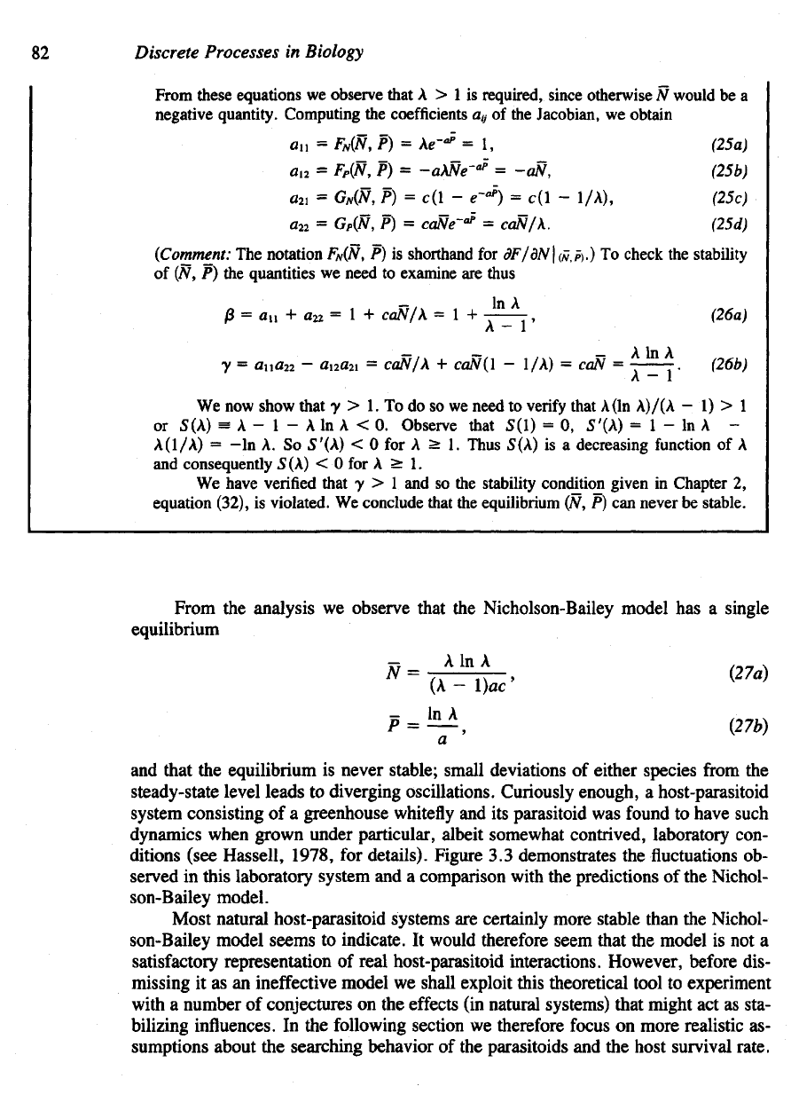
Nicholson-Bailey equations:
We now
analyze this model using
the
methods developed
in
Chapter
2. The
steps
include:
1.
Solving
for
steady states.
2.
Finding
the
coefficients
of the
Jacobian matrix (for
the
system linearized about
the
steady
state).
3.
Checking
the
stability condition derived
in
Section 2.8.
Solving
for
steady
states,
we
obtain
the
trivial
solution
N = 0, or
These
imply
that
82
Discrete Processes
in
Biology
From these equations
we
observe that
A > 1 is
required, since otherwise
N
would
be a
negative quantity. Computing
the
coefficients
a
ti
of the
Jacobian,
we
obtain
From
the
analysis
we
observe that
the
Nicholson-Bailey model
has a
single
equilibrium
(Comment:
The
notation
F
N
(N,
P) is
shorthand
for
#F/dN\
&,?).)
To
check
the
stability
of
(N, P) the
quantities
we
need
to
examine
are
thus
We
now
show that
y > 1. To do so we
need
to
verify
that
A
(In
A)/(A
- 1) > 1
or
5(A)
=
A-l-AlnA<0.
Observe that
S(l)
= 0,
S'(\)
= 1 - In
A
-
A
(I/A)
= -In A. So
5'(A)
< 0 for A > 1.
Thus
5(A)
is a
decreasing
function
of A
and
consequently
5
(A)
< 0 for A ^ 1.
We
have verified that
y > 1 and so the
stability condition given
in
Chapter
2,
equation
(32),
is
violated.
We
conclude that
the
equilibrium
(N, P) can
never
be
stable.
and
that
the
equilibrium
is
never
stable;
small deviations
of
either species
from
the
steady-state level
leads
to
diverging oscillations. Curiously enough,
a
host-parasitoid
system consisting
of a
greenhouse
whitefly
and its
parasitoid
was
found
to
have such
dynamics when grown under particular, albeit somewhat contrived, laboratory con-
ditions (see Hassell, 1978,
for
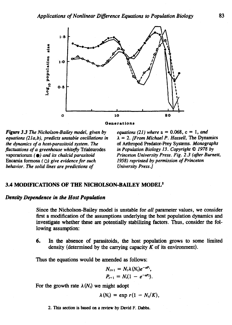
details). Figure
3.3
demonstrates
the fluctuations ob-
served
in
this laboratory system
and a
comparison
with
the
predictions
of the
Nichol-
son-Bailey model.
Most natural host-parasitoid systems
are
certainly more stable than
the
Nichol-
son-Bailey model seems
to
indicate.
It
would therefore seem that
the
model
is not a
satisfactory
representation
of
real
host-parasitoid interactions. However, before dis-
missing
it as an
ineffective model
we
shall exploit this theoretical tool
to
experiment
with
a
number
of
conjectures
on the
effects
(in
natural systems) that might
act as
sta-
bilizing influences.
In the
following section
we
therefore
focus
on
more realistic
as-
sumptions
about
the
searching behavior
of the
parasitoids
and the
host survival rate.
Applications
of
Nonlinear
Difference
Equations
to
Population
Biology
83
Figure
3.3 The
Nicholson-Bailey model, given
by
equations (21a,b), predicts unstable oscillations
in
the
dynamics
of a
host-parasitoid system.
The
fluctuations
of
a
greenhouse
whitefly
Trialeurodes
vaporariorum
(o ) and its
chalcid parasitoid
Encarsia
formosa
(o)
give evidence
for
such
behavior.
The
solid lines
are
predictions
of
equations
(21) where
a =
0.068,
c = 1, and
A
= 2.
[From Michael
P.
Hassell,
The
Dynamics
of
Arthropod
Predator-Prey
Systems.
Monographs
in
Population Biology
13.
Copyright
©
7975
by
Princeton University
Press.
Fig.
2.3
(after
Burnett,
1958)
reprinted
by
permission
of
Princeton
University
Press.]
3.4
MODIFICATIONS
OF THE
NICHOLSON-BAILEY MODEL
2
Density
Dependence
in the
Host
Population
Since
the
Nicholson-Bailey model
is
unstable
for all
parameter values,
we
consider
first a
modification
of the
assumptions underlying
the
host population dynamics
and
investigate whether these
are
potentially stabilizing factors. Thus, consider
the
fol-
lowing assumption:
6. In the
absence
of
parasitoids,
the
host population grows
to
some limited
density (determined
by the
carrying capacity
K of its
environment).
Thus
the
equations would
be
amended
as
follows:
2.
This section
is
based
on a
review
by
David
F.
Dabbs.
For the
growth rate
A(/V,)
we
might adopt
84
Discrete
Processes
in
Biology
as
in
equation (8). Thus
if P = 0, the
host population grows
up to
density
M = K
and
declines
if N, > K. The
revised model
is
This
model
was
studied
in
some detail
by
Beddington
et al.
(1975). They
found
it
convenient
to
discuss
its
behavior
in
terms
of the
quantity
q
where
q = N/K = the
ratio
of
steady-state host density with
and
without parasitoids
present.
The
value
of q
indicates
to
what extent
the
steady-state population
is
depressed
by
the
presence
of
parasitoids.
Equations (28a,b)
are
sufficiently
Complicated that
it is
impossible
to
derive
explicit expressions
for the
states
N and P.
However, these
can be
expressed
in
terms
of
q and P as
follows:
It
transpires that
the
resulting model
is
stable
for a
fairly
wide range
of
realistic
parameter values,
as
desired.
Even
so, the
return
to
equilibrium
in
these ranges
is
typically rather complex.
As
parameters
are
changed,
the
equilibrium does lose
its
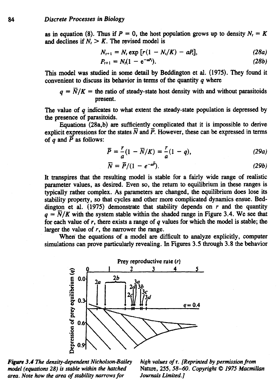
stability property,
so
that cycles
and
other more complicated dynamics ensue. Bed-
dington
et al.
(1975)
demonstrate that stability depends
on r and the
quantity
q = N/K
with
the
system stable within
the
shaded range
in
Figure 3.4.
We see
that
for
each value
of r,
there exists
a
range
of q
values
for
which
the
model
is
stable;
the
larger
the
value
of r, the
narrower
the
range.
When
the
equations
of a
model
are
difficult
to
analyze explicitly, computer
simulations
can
prove particularly revealing.
In
Figures
3.5
through
3.8 the
behavior
Figure
3.4 The
density-dependent
Nicholson-Bailey
model
(equations
28) is
stable within
the
hatched
area.
Note
how the
area
of
stability
narrows
for
high
values ofr.
[Reprinted
by
permission
from
Nature, 255,
58-60.
Copyright
©
1975 Macmillan
Journals
Limited.]
Applications
of
Nonlinear
Difference
Equations
to
Population
Biology
85
of
solutions
to
equations (28a,b) obtained
with
a
simple computer simulation
are
dis-
played
for a
variety
of
parameter
choices.
A
TURBO
-
PASCAL program, written
by
David
F.
Dabbs
and run on a
personal computer,
was
used
to
generate successive
values
of N, and P, and to
plot these simultaneously. What
is
somewhat novel about
these
plots
is
that
in
this two-variable system, time
is
suppressed
and
(N,,
Pt)
values
are
plotted
in the
plane sometimes referred
to as the NP
phase plane.
(In a
later
chapter
a
similar technique will
be
applied
to
systems
of two
differential
equations
in
two
variables.)
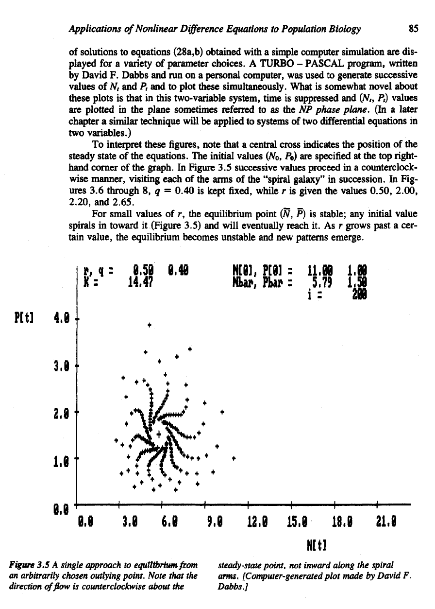
To
interpret these
figures,
note that
a
central cross indicates
the
position
of the
steady state
of the
equations.
The
initial values (No,
Po) are
specified
at the top right-
hand
corner
of the
graph.
In
Figure
3.5
successive values proceed
in a
counterclock-
wise manner, visiting each
of the
arms
of the
"spiral
galaxy"
in
succession.
In
Fig-
ures
3.6
through
8, q =
0.40
is
kept
fixed,
while
r is
given
the
values 0.50, 2.00,
2.20,
and
2.65.
For
small values
of r, the
equilibrium point
(N, P) is
stable;
any
initial value
spirals
in
toward
it
(Figure 3.5)
and
will eventually reach
it. As r
grows past
a
cer-
tain
value,
the
equilibrium becomes unstable
and new
patterns emerge.
Figure
3.5 A
single approach
to
equilibrium/com
steady-state
point,
not
inward along
the
spiral
an
arbitrarily chosen outlying
point.
Note that
the
arms.
(Computer-generated
plot
made
by
David
F.
direction
of flow is
counterclockwise about
the
Dabbs
]
