Edelstein-Keshet L. Mathematical Models in Biology
Подождите немного. Документ загружается.

46
Discrete
Processes
in
Biology
In
example
2 of
Section
2.2 we
showed that equation (11)
has two
possible
steady
states,
only
one of
which
is
nontrivial (nonzero):
x
2
= 1 -
1/r.
The
steady
state
is
stable only when
the
parameter
r
satisfies
1 < r < 3.
(Notice that
the
parameter
d in
equation (12) only influences scaling
of the
qualitative behavior.)
What
happens beyond
the
value
of r = 3 and up to the
permitted maximal
value
of r? Let us
cautiously turn
the
knob
on our
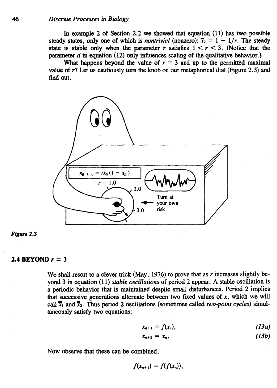
metaphorical dial (Figure 2.3)
and
find
out.
Figure
2.3
2.4
BEYOND
r = 3
We
shall resort
to a
clever trick (May, 1976)
to
prove that
as r
increases slightly
be-
yond
3 in
equation (11) stable oscillations
of
period
2
appear.
A
stable oscillation
is
a
periodic behavior that
is
maintained despite small disturbances. Period
2
implies
that
successive generations alternate between
two fixed
values
of x,
which
we
will
call
xi and
X2.
Thus period
2
oscillations (sometimes called
two-point
cycles)
simul-
taneously
satisfy
two
equations:
Now
observe that these
can be
combined,
Nonlinear
Difference
Equations
47
and
a
steady state
of
equation (15),
x (or a fixed
point
of g), is
really
a
period
2
solu-
tion
of
(13a). Note that there must
be two
such values,
*i and *2
since
by
assumption
*
oscillates
between
two fixed
values.
By
this trick
we
have reduced
the new
problem
to one
with which
we are fa-
miliar. That
is,
stability
of a
period
2
oscillation
can be
determined
by
using
the
methods
of
Section
2.2 on
equation (15).
Briefly,
suppose
an
initial situation
is
cre-
ated whereby
XQ
= x\ + eo,
where
€o is a
small quantity. Stability
of *i
implies that
periodic behavior will
be
reestablished, i.e., that
the
deviation
€Q
from
this behavior
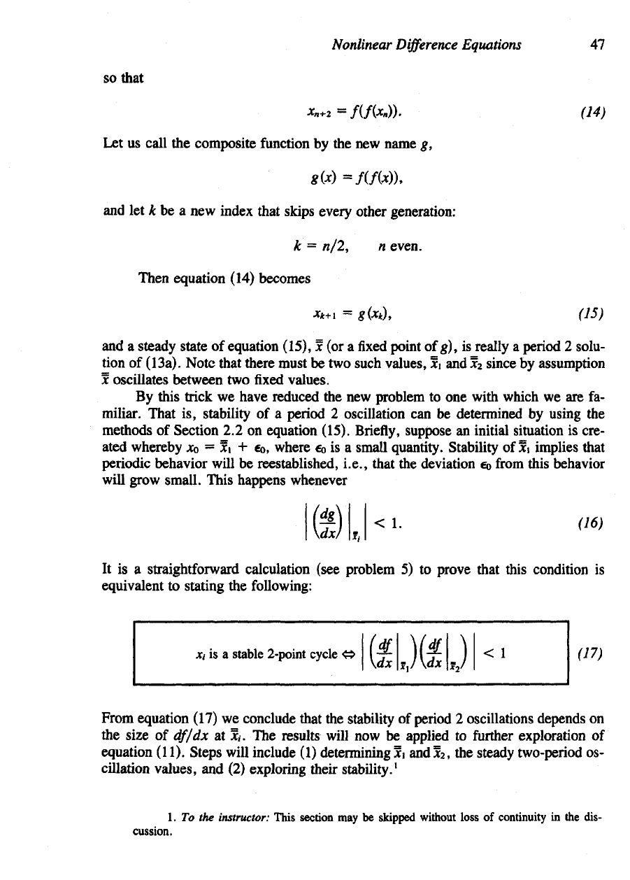
will grow small. This happens whenever
It
is a
straightforward calculation (see problem
5) to
prove that this condition
is
equivalent
to
stating
the
following:
From equation (17)
we
conclude that
the
stability
of
period
2
oscillations depends
on
the
size
of
df/dx
at *,. The
results will
now be
applied
to
further
exploration
of
equation (11). Steps will include
(1)
determining
x\ and *2, the
steady two-period
os-
cillation
values,
and (2)
exploring their stability.
1
so
that
Let us
call
the
composite
function
by the new
name
g,
and
let k be a new
index that skips every other generation:
Then equation (14)
becomes
1. To the
instructor: This section
may be
skipped without loss
of
continuity
in the
dis-
cussion.
xi
is a
stable 2-point cycle
48
Discrete Processes
in
Biology
Ctxumjfiv
j _
Find
jci
and x
2
for the
two-point cycles
of
equation (11).
Solution
To do so, first
determine
the
composite
map
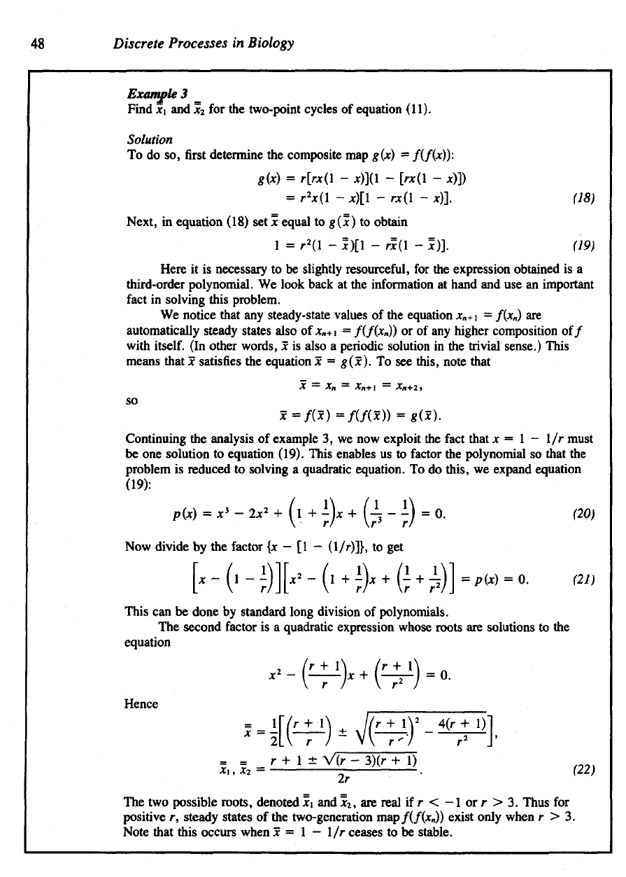
g(x)
=
/(/(*)):
Next,
in
equation (18)
set x
equal
to
g(x)
to
obtain
Here
it is
necessary
to be
slightly resourceful,
for the
expression obtained
is a
third-order polynomial.
We
look back
at the
information
at
hand
and use an
important
fact
in
solving this problem.
We
notice that
any
steady-state values
of the
equation x
n
+\
=
/(*„)
are
automatically steady states also
of
x
n
+
1
=
/(/(*„))
or of any
higher composition
of/
with
itself.
(In
other words,
x is
also
a
periodic solution
in the
trivial sense.) This
means that
x
satisfies
the
equation
x =
g(x).
To see
this,
note that
so
Continuing
the
analysis
of
example
3, we now
exploit
the
fact
that
x = 1 - 1/r
must
be one
solution
to
equation (19). This enables
us to
factor
the
polynomial
so
that
the
problem
is
reduced
to
solving
a
quadratic equation.
To do
this,
we
expand equation
(19):
Now
divide
by the
factor
{x
—
[1 -
(1/r)]},
to get
This
can be
done
by
standard long division
of
polynomials.
The
second
factor
is a
quadratic
expression
whose
roots
are
solutions
to the
equation
Hence
The
two
possible
roots,
denoted
x\ and *
2
, are
real
if r <
—
1 or r > 3.
Thus
for
positive
r,
steady
states
of the
two-generation
map f
f(f(xn))
exist only when
r > 3.
Note that this occurs when
x = I — 1/r
ceases
to be
stable.
Nonlinear
Difference
Equations
49
With
xi and x
2
computed,
it is a
straightforward (albeit algebraically messy)
task
to
test their stability.
To do so, it is
necessary
to
compute
(df/dx)
and
evaluate
at
the
values
x\ and x
2
.
When this
is
done,
we
obtain
a
second range
of
behavior: sta-
bility
of the
two-point cycles
for 3 < r < r
2
with
r
2
=
3.3. Again
we
could pose
the
question, What happens beyond
r = r
2
?
It
should
be
emphasized that
the
trick used
in
exploring period
2
oscillations
could
be
used
for any
higher period
n: n = 3, 4
Because
the
analysis
be-
comes increasingly cumbersome, this method will
not be
further
applied. Instead,
we
will explore some underlying geometric ideas that make
the
process
of
"tuning"
a
parameter more immediately significant.
2.5
GRAPHICAL METHODS
FOR
FIRST-ORDER EQUATIONS
In
this section
we
examine
a
simple technique
for
visualizing
the
solutions
of first-
order
difference equations that
can be
used
for
gaining insight into
the
stability
of
steady states
and the
effects
of
parameter variations.
As an
example, consider equa-
tion (11).
Let us
draw
a
graph
of f
(x),
the
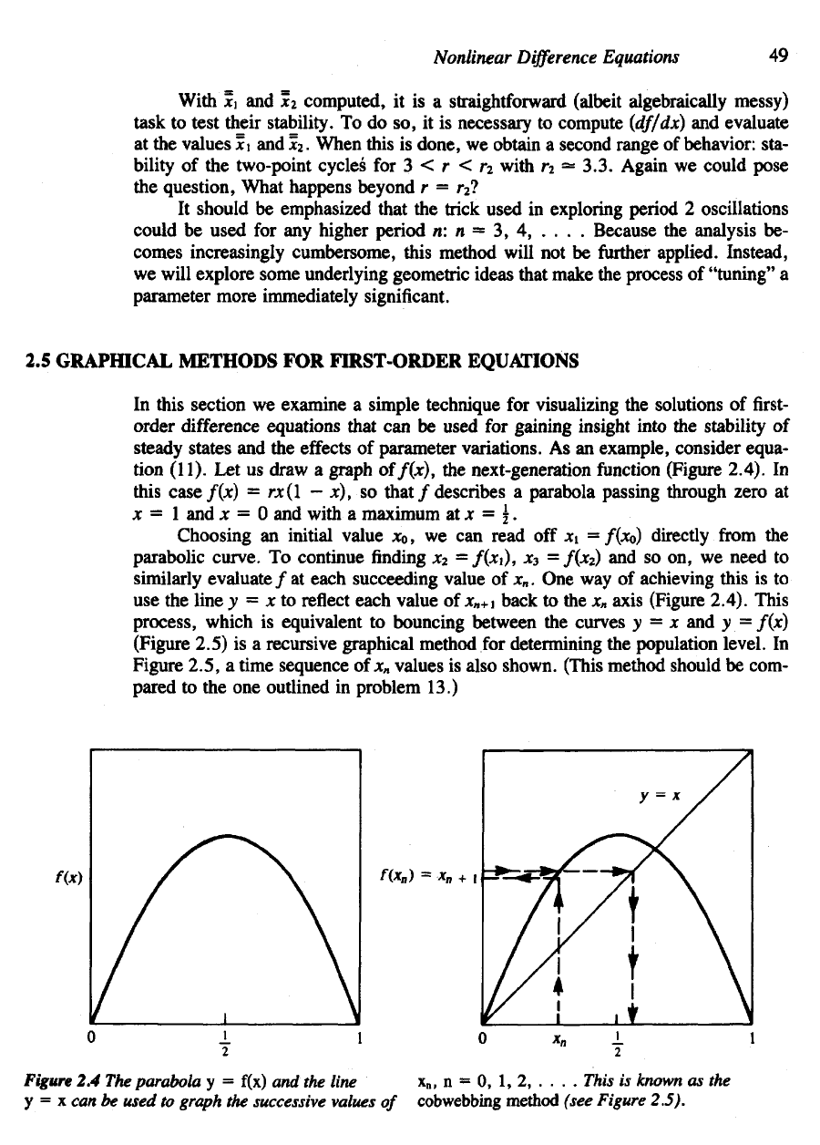
next-generation function (Figure 2.4).
In
this
case f(x)
=
rjc(l
- x), so
that
/
describes
a
parabola passing through zero
at
x
= 1 and x = 0 and
with
a
maximum
at x = J.
Choosing
an
initial value
XQ, we can
read
off
JCi
=
/(xo) directly
from
the
parabolic
curve.
To
continue finding
*
2
=
/(*i),
jc
3
=
/(*
2
)
and so on, we
need
to
similarly
evaluate
/ at
each succeeding value
of
jc
n
.
One way of
achieving this
is to
use the
line
y = x to
reflect
each value
of
x
n
+\
back
to the x*
axis (Figure 2.4). This
process,
which
is
equivalent
to
bouncing between
the
curves
y = x and y
=/(*)
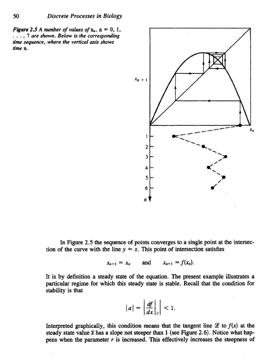
(Figure 2.5)
is a
recursive graphical method
for
determining
the
population level.
In
Figure 2.5,
a
time sequence
of
x»
values
is
also shown. (This method should
be
com-
pared
to the one
outlined
in
problem 13.)
Figure
2.4 The
parabola
y =
f(x)
and the
line
x
n
, n = 0, 1, 2, . . . .
This
is
known
as the
y
= x can be
used
to
graph
the
successive values
of
cobwebbing method (see Figure 2.5).
50
Discrete Processes
in
Biology
Figure
2.5 A
number
of
values ofx
a
,
n = 0, 1,
. . . , 7 are
shown. Below
is the
corresponding
time
sequence, where
the
vertical axis shows
time n.
In
Figure
2.5 the
sequence
of
points
converges
to a
single
point
at the
intersec-
tion
of the
curve with
the
line
y = x.
This point
of
intersection satisfies
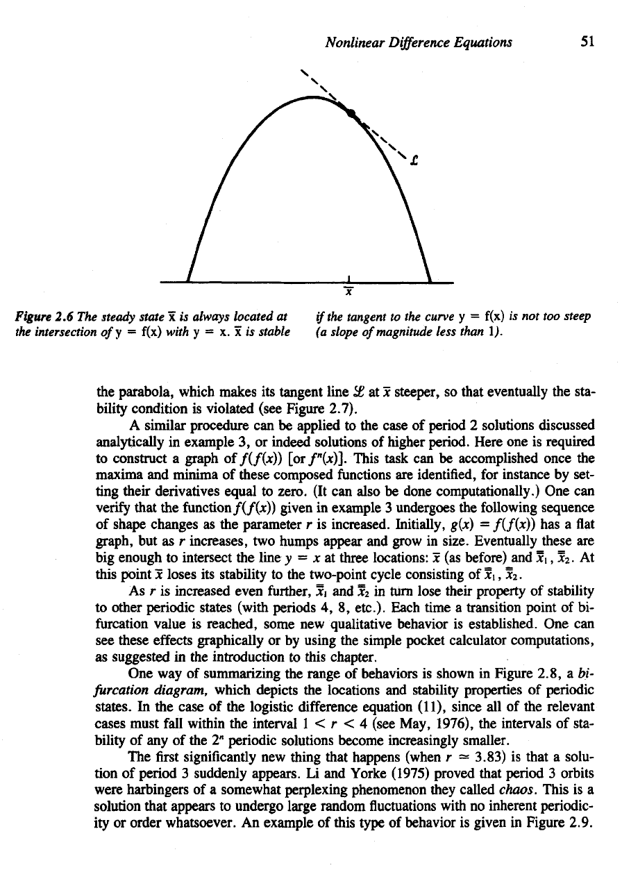
Interpreted graphically, this condition means that
the
tangent line
££ to
f(x)
at the
steady state value
x has a
slope
not
steeper
than
1
(see Figure 2.6). Notice what hap-
pens when
the
parameter
r is
increased. his effectively increases
the
steepness
of
It
is by
definition
a
steady state
of the
equation.
The
present example illustrates
a
particular regime
for
which this steady state
is
stable. Recall that
the
condition
for
stability
is
that
Nonlinear
Difference
Equations
51
Figure
2.6 The
steady
state
x is
always
located
at
if
the
tangent
to the
curve
y =
f(x)
is not too
steep
the
intersection
ofy =
f(x) with
y = x. x is
stable
(a
slope
of
magnitude
less than
I).
the
parabola, which makes
its
tangent line
X at x
steeper,
so
that eventually
the
sta-
bility
condition
is
violated
(see Figure 2.7).
A
similar procedure
can be
applied
to the
case
of
period
2
solutions discussed
analytically
in
example
3, or
indeed solutions
of
higher period. Here
one is
required
to
construct
a
graph
of
/(/(*))
[or/"(*)].
This task
can be
accomplished once
the
maxima
and
minima
of
these composed
functions
are
identified,
for
instance
by
set-
ting
their derivatives equal
to
zero.
(It can
also
be
done computationally.)
One can
verify
that
the
function
/(/(*))
given
in
example
3
undergoes
the
following sequence
of
shape changes
as the
parameter
r is
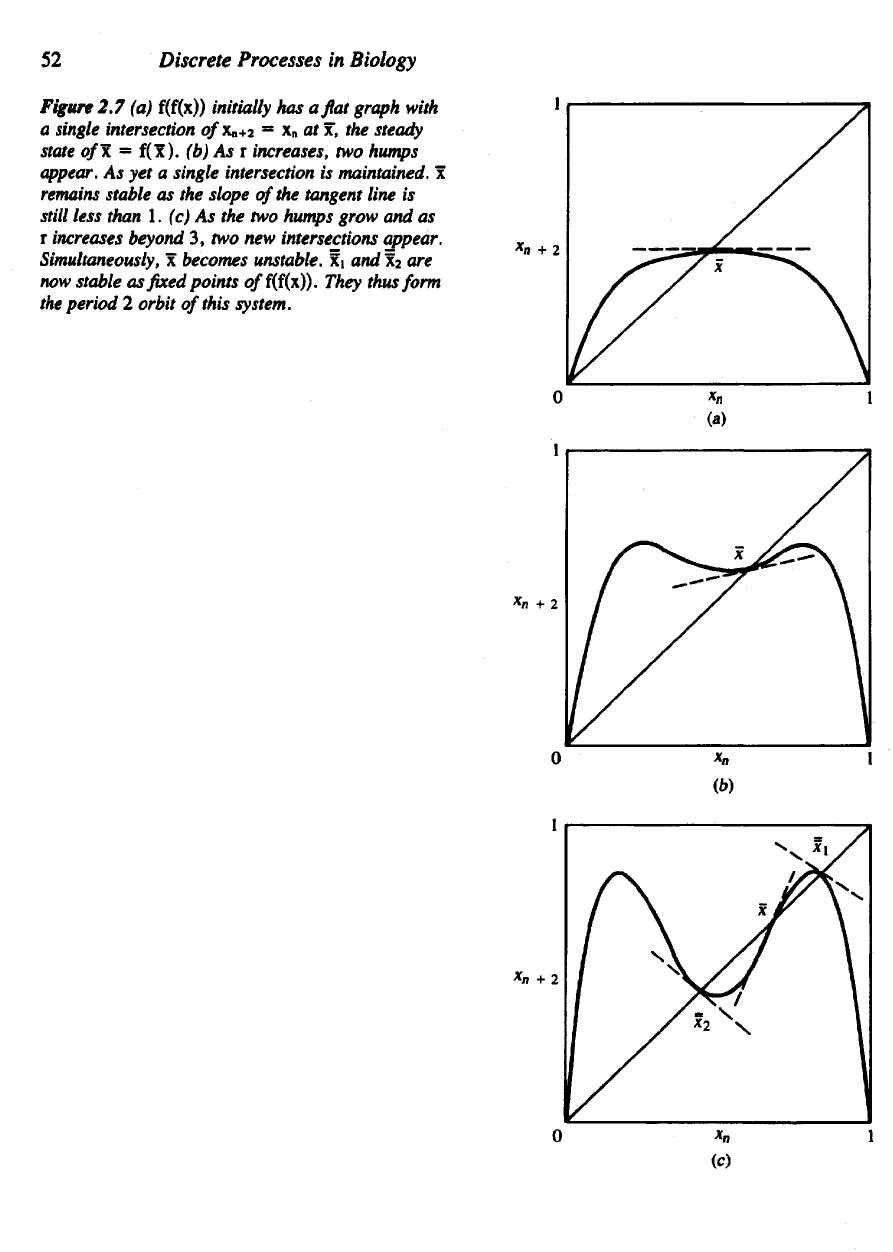
increased. Initially, g(x)
=
f(f(x})
has a flat
graph,
but as r
increases,
two
humps appear
and
grow
in
size. Eventually these
are
big
enough
to
intersect
the
line
y = x at
three locations:
x (as
beforehand
*i,
jc
2
.
At
this point
x
loses
its
stability
to the
two-point cycle consisting
of *
i,
xi.
As r is
increased even further,
x\ and
jc2
in
turn
lose
their property
of
stability
to
other
periodic
states (with periods
4, 8,
etc.).
Each time
a
transition point
of bi-
furcation
value
is
reached, some
new
qualitative behavior
is
established.
One can
see
these effects graphically
or by
using
the
simple pocket calculator computations,
as
suggested
in the
introduction
to
this chapter.
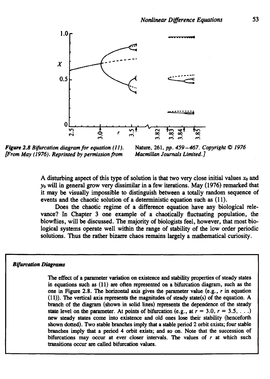
One way of
summarizing
the
range
of
behaviors
is
shown
in
Figure 2.8,
a bi-
furcation
diagram, which depicts
the
locations
and
stability properties
of
periodic
states.
In the
case
of the
logistic difference equation (11), since
all of the
relevant
cases
must
fall
within
the
interval
1 < r < 4
(see May,
1976),
the
intervals
of
sta-
bility
of any of the 2"
periodic solutions become increasingly smaller.
The first
significantly
new
thing that happens
(when
r —
3.83)
is
that
a
solu-
tion
of
period
3
suddenly appears.
Li and
Yorke (1975) proved that period
3
orbits
were harbingers
of a
somewhat perplexing phenomenon they called chaos. This
is a
solution that appears
to
undergo large random
fluctuations
with
no
inherent periodic-
ity
or
order whatsoever.
An
example
of
this type
of
behavior
is
given
in
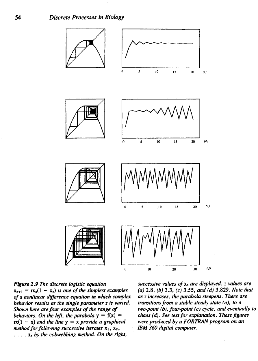
Figure 2.9.
52
Discrete
Processes
in
Biology
Figure
2.7 (a)
f(f(x)) initially
has
aflat graph with
a
single intersection
of
x
n
+
2
= x
n
at x, the
steady
state
of\ =
f(x).
(b) As r
increases,
two
humps
appear.
As yet a
single intersection
is
maintained,
x
remains
stable
as the
slope
of
the
tangent line
is
still
less than
1. (c) As the two
humps grow
and as
T
increases beyond
3, two new
intersections appear.
Simultaneously,
x
becomes unstable,
f
i
and x
2
are
now
stable
as fixed
points
off(f(\)).
They
thus form
the
period
2
orbit
of
this system.
Nonlinear
Difference
Equations
53
Figure
2.8
Bifurcation
diagram
for
equation
(11).
[From
May
(1976).
Reprinted
by
permission
from
Nature,
261,
pp.
459-467.
Copyright
©
7976
Macmillan
Journals
Limited.]
A
disturbing aspect
of
this type
of
solution
is
that
two
very close initial values
x
0
and
yo
will
in
general grow very dissimilar
in a few
iterations.
May
(1976) remarked
that
it may be
visually impossible
to
distinguish between
a
totally random sequence
of
events
and the
chaotic solution
of a
deterministic equation such
as
(11).
Does
the
chaotic regime
of a
difference
equation have
any
biological rele-
vance?
In
Chapter
3 one
example
of a
chaotically
fluctuating
population,
the
blowflies,
will
be
discussed.
The
majority
of
biologists feel, however,
mat
most bio-
logical
systems operate well within
the
range
of
stability
of the low
order
periodic
solutions. Thus
the
rather bizarre chaos remains largely
a
mathematical curiosity.
Bifurcation
Diagrams
The
effect
of a
parameter variation
on
existence
and
stability properties
of
steady states
in
equations such
as
(11)
are
often
represented on a
bifurcation
diagram, such
as the
one in
Figure
2.8.
The
horizontal axis gives
the
parameter value (e.g.,
r in
equation
(11)).
The
vertical axis
represents the
magnitudes
of
steady state(s)
of the
equation.
A
branch
of the
diagram (shown
in
solid lines)
represents the
dependence
of the
steady
state level
on the
parameter.
At
points
of
bifurcation
(e.g.,
at r —
3.0,
r =
3.5,
. . .)
new
steady states come into existence
and old
ones lose their stability (henceforth
shown
dotted).
Two
stable branches imply
that
a
stable period
2
orbit
exists;
four
stable
branches imply that
a
period
4
orbit exists;
and so on.
Note that
the
succession
of
bifurcations
may
occur
at
ever closer intervals.
The
values
of r at
which
such
transitions occur
are
called
bifurcation values.
54
Discrete
Processes
in
Biology
Figure
2.9 The
discrete logistic equation
x
n
+i
=
rx
n
(l
- x
n
)
is-one
of
the
simplest examples
of
a
nonlinear
difference
equation
in
which complex
behavior
results
as the
single parameter
r is
varied.
Shown
here
are
four examples
of
the
range
of
behaviors.
On the
left,
the
parabola
y =
f(x)
=
rx(l
- x)
and
the
line
y =
\provide
a
graphical
method
for
following successive iterates
\\,
X2,
. . . , x
n
by the
cobwebbing method.
On the
right.
su ive
values
of
x
n
are
displayed,
r
values
are
(a)
2.8,
(b)
3.3,
(c)
3.55,
and (d)
3.829.
Note that
as r
increases,
the
parabola steepens. There
are
transitions
from
a
stable steady state
(a),
to a
two-point
(b), four-point
(c)
cycle,
and
eventually
to
chaos
(d).
See
text
for
explanation. These
figures
were
produced
by a
FORTRAN
program
on an
IBM
360
digital computer.
Nonlinear
Difference
Equations
55
Summary
and
Applications
of the
Logistic
Difference
Equation
(11)
Equation
(11)
has
been used
as a
convenient example
for
illustrating
a
number
of key
ideas.
First,
we saw
that
the
number
of
parameters
affecting
the
qualitative
features
of a
model
may be
smaller
than
the
number
that
initially appear. Further,
we
observed
that
existence
and
stability
of
steady states
and
periodic solutions changed
as the
critical
parameter
was
varied
(or
"tuned"). Finally,
we had a
brief exposure
to the
fact
that
difference
equations
can
produce somewhat
unusual
solutions quite
unlike
their "fame"
continuous
counterparts.
Equation
(11)
is
seldom used
as an
honest-to-goodness biological model.
However,
it
serves
as a
useful
pedagogical example
of
calculations
and
results
that
also
hold
for
other, more realistic models, some
of
which
will
be
described
in
Chapter
3.
For a
more detailed
and
thorough analysis
of
this equation,
turn
to the
lucid
review
by
May
(1976).
2.6 A
WORD ABOUT
THE
COMPUTER
Perhaps
one of the
most pleasing
properties
of
difference equations
is
that they read-
ily
yield
to
numerical exploration, whether
by
calculator
or
with
a
digital computer.
This property
is not
shared with
the
continuous
differential
equations. Solutions
to
difference
equations
are
obtainable
by
sequential arithmetic operations,
a
task
for
which
the
computer
is
precisely suited. Indeed,
the key
strategy
in
tackling
the
more
problematic differential equations
by
numerical computations
is to
find
a
reliable
ap-
proximating difference equation
to
solve instead. This makes
it
particularly impor-
tant
to
appreciate
the
properties
and
eccentricities
of
these equations.
2.7
SYSTEMS
OF
NONLINEAR DIFFERENCE EQUATIONS
To
conclude this chapter,
we
will extend
the
methods developed
for
single equations
to
systems
of n
difference equations
for
arbitrary
n. For
simplicity
of
notation
we
will discuss here
the
case
where
n = 2.
Assume therefore that
two
independent vari-
ables
x and v are
related
by the
system
of
equations
where/and
g are
nonlinear functions. Steady-state values
x and y
satisfy
We now
explore
the
stability
of
these steady states
by
analyzing
the
fate
of
small deviations.
As
before, this will result
in a
linearized system
of
equations
for
