Edelstein-Keshet L. Mathematical Models in Biology
Подождите немного. Документ загружается.

126
Continuous Processes
and
Ordinary
Differential
Equations
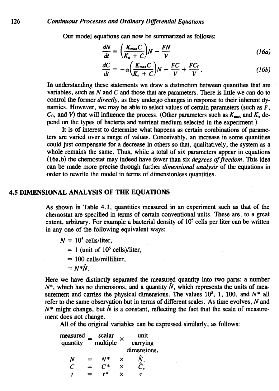
Our
model equations
can now be
summarized
as
follows:
In
understanding these statements
we
draw
a
distinction between quantities that
are
variables, such
as N and C and
those that
are
parameters. There
is
little
we can do to
control
the
former directly,
as
they undergo changes
in
response
to
their inherent
dy-
namics. However,
we may be
able
to
select values
of
certain parameters
(such
as F,
Co,
and V)
that will
influence
the
process. (Other parameters such
as
/ifmax
and K
n
de-
pend
on the
types
of
bacteria
and
nutrient medium selected
in the
experiment.)
It
is of
interest
to
determine what happens
as
certain combinations
of
parame-
ters
are
varied over
a
range
of
values. Conceivably,
an
increase
in
some quantities
could just compensate
for a
decrease
in
others
so
that, qualitatively,
the
system
as a
whole remains
the
same. Thus, while
a
total
of six
parameters appear
in
equations
(16a,b)
the
chemostat
may
indeed have
fewer
than
six
degrees
of
freedom.
This idea
can be
made more precise through
further
dimensional analysis
of the
equations
in
order
to
rewrite
the
model
in
terms
of
dimensionless quantities.
4.5
DIMENSIONAL ANALYSIS
OF THE
EQUATIONS
As
shown
in
Table 4.1, quantities measured
in an
experiment such
as
that
of the
chemostat
are
specified
in
terms
of
certain conventional units. These are,
to a
great
extent, arbitrary.
For
example
a
bacterial density
of 10
5
cells
per
liter
can be
written
in
any one of the
following equivalent ways:
Here
we
have distinctly separated
the
measured quantity into
two
parts:
a
number
'N*,
which
has no
dimensions,
and a
quantity
N,
which represents
the
units
of
mea-
surement
and
carries
the
physical dimensions.
The
values 10
5
,
1,
100,
and N* all
refer
to the
same observation
but in
terms
of
different
scales.
As
time evolves,
N and
A
N*
might change,
but N is a
constant, reflecting
the
fact
that
the
scale
of
measure-
ment
does
not
change.
All
of the
original
variables
can be
expressed
similarly,
as
follows:
An
Introduction
to
Continuous
Models
127
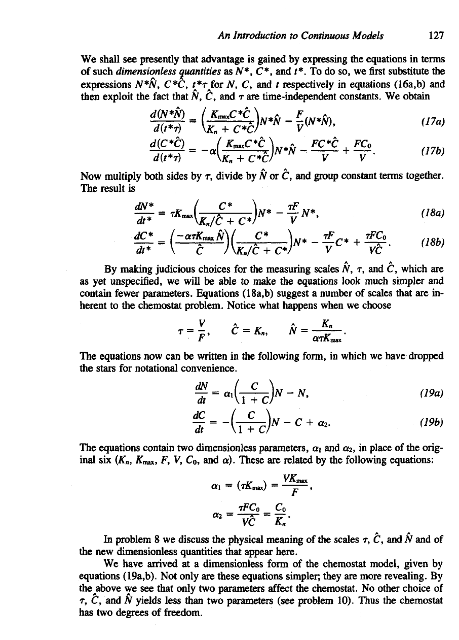
We
shall
see
presently that advantage
is
gained
by
expressing
the
equations
in
terms
of
such dimensionless quantities
asN*,C*,
and t*. To do so, we first
substitute
the
expressions
N*N, C*C,
f*T
A
for
N, C, and t
respectively
in
equations
(16a,b)
and
then exploit
the
fact that
N, C, and T are
time-independent constants.
We
obtain
Now
multiply both sides
by T,
divide
by
W
or C, and
group constant terms together.
The
result
is
/\
^
By
making judicious choices
for the
measuring scales
N, T, and C,
which
are
as yet
unspecified,
we
will
be
able
to
make
the
equations look
much
simpler
and
contain
fewer
parameters. Equations (18a,b) suggest
a
number
of
scales that
are in-
herent
to the
chemostat problem. Notice what happens when
we
choose
The
equations
now can be
written
in the
following
form,
in
which
we
have dropped
the
stars
for
notational convenience.
The
equations contain
two
dimensionless parameters,
a\ and a
2
, in
place
of the
orig-
inal
six
(K
n
,
£max,
F, V, Co, and a).
These
are
related
by the
following equations:
In
problem
8 we
discuss
the
physical meaning
of the
scales
T, C, and N and of
the new
dimensionless quantities
mat
appear here.
We
have arrived
at a
dimensionless
form
of the
chemostat model, given
by
equations (19a,b).
Not
only
are
these equations simpler; they
are
more revealing.
By
thejabove
we see
that only
two
parameters
affect
the
chemostat.
No
other
choice
of
T,
C, and N
yields
less
than
two
parameters (see problem 10). Thus
the
chemostat
has two
degrees
of
freedom.
128
Continuous Processes
and
Ordinary
Differential
Equations
Equations
(19a,b)
are
nonlinear because
of the
term NC/(l
+ C).
Generally
this means that there
is
little hope
of finding
explicit analytic solutions
for
N(t)
and
C(i).
However,
we can
still
explore
the
nature
of
special classes
of
solutions, just
as
we
did in the
nonlinear difference-equation models. Since
we are
interested
in
main-
taining
a
continuous culture
in
which bacteria
and
nutrients
are
present
at
some
fixed
densities,
we
will next determine whether equations (19a,b) admit
a
steady-state
so-
lution
of
this type.
4.6
STEADY-STATE SOLUTIONS
A
steady state
is a
situation
in
which
the
system does
not
appear
to
undergo
any
change.
To be
more
precise,
the
values
of
state variables, such
as
bacterial density
and
nutrient concentration
within
the
chemostat, would
be
constant
at
steady state
even though individual nutrient particles continue
to
enter, leave,
or be
consumed.
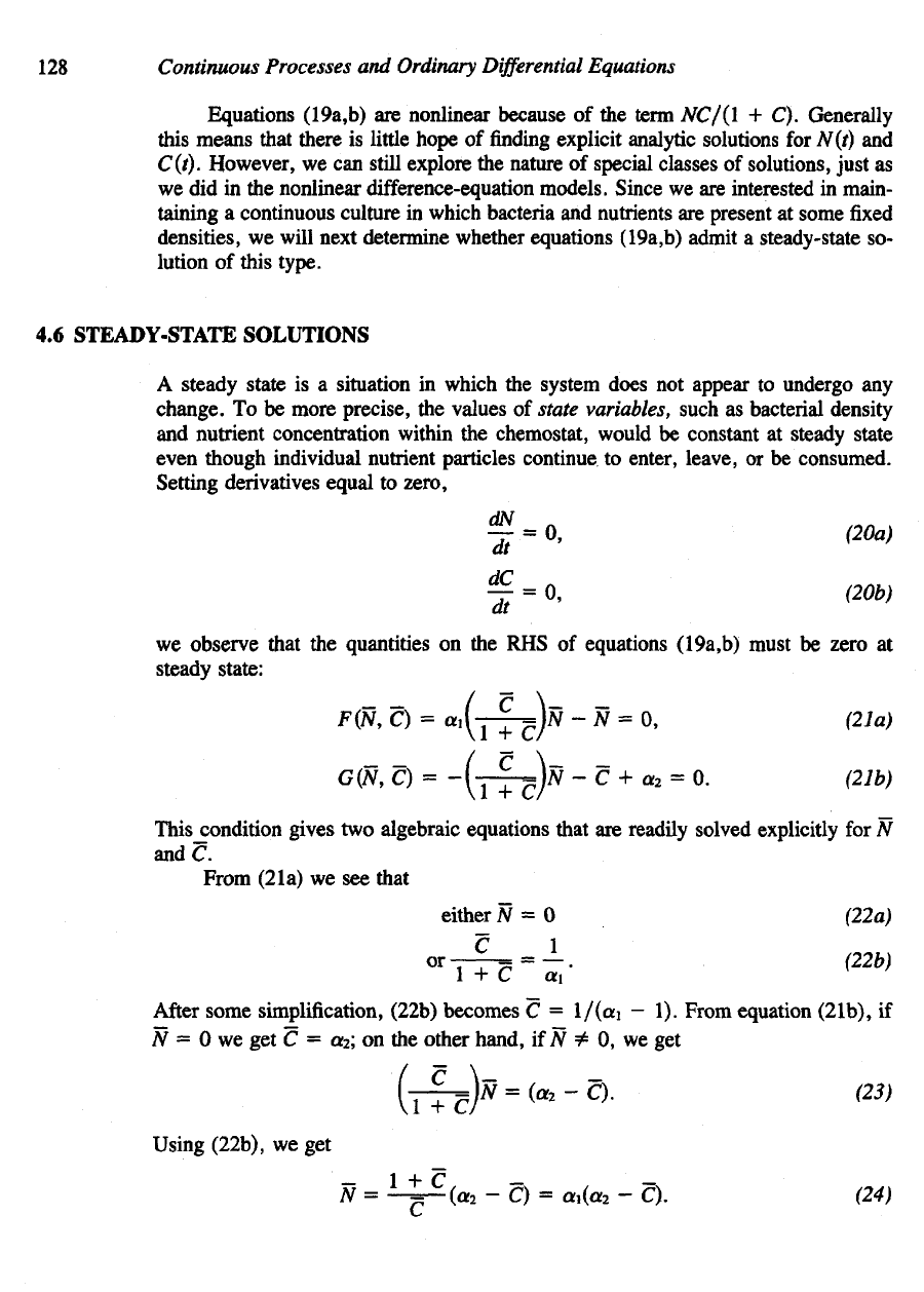
Setting derivatives equal
to
zero,
we
observe that
the
quantities
on the RHS of
equations (19a,b)
must
be
zero
at
steady
state:
This_condition
gives
two
algebraic equations that
are
readily solved explicitly
for N
andC.
From (2la)
we see
that
After
some simplification, (22b)
becomes
C =
\/(a\
— 1).
From equation
(21b),
if
N
= 0 we get C = a
2
; on the
other
hand,
if N
=£
0, we get
Using
(22b),
we get
An
Introduction
to
Continuous
Models
129
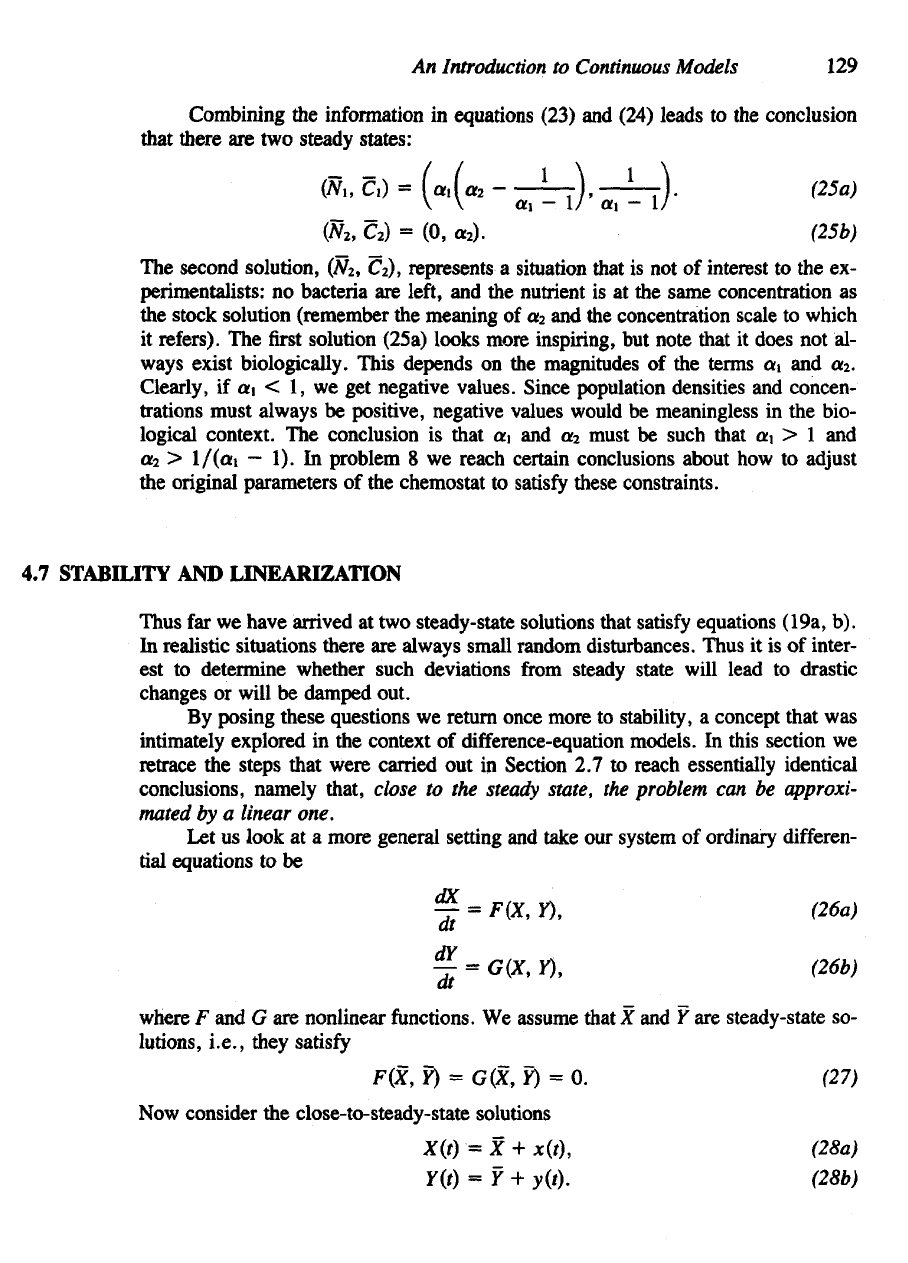
Combining
the
information
in
equations (23)
and
(24) leads
to the
conclusion
that there
are two
steady
states:
4.7
STABILITY
AND
LINEARIZATION
Thus
far we
have arrived
at two
steady-state solutions that
satisfy
equations (19a,
b).
In
realistic situations there
are
always small random disturbances. Thus
it is of
inter-
est to
determine whether such deviations
from
steady state will lead
to
drastic
changes
or
will
be
damped out.
By
posing these questions
we
return once more
to
stability,
a
concept that
was
intimately
explored
in the
context
of
difference-equation
models.
In
this section
we
retrace
the
steps that were carried
out in
Section
2.7 to
reach essentially identical
conclusions, namely that,
close
to the
steady
state,
the
problem
can be
approxi-
mated
by a
linear one.
Let us
look
at a
more general setting
and
take
our
system
of
ordinary differen-
tial equations
to be
The
second solution, (N2, C2), represents
a
situation that
is not of
interest
to the ex-
perimentalists:
no
bacteria
are
left,
and the
nutrient
is at the
same concentration
as
the
stock solution (remember
the
meaning
of a
2
and the
concentration scale
to
which
it
refers).
The first
solution (25a) looks more inspiring,
but
note that
it
does
not al-
ways
exist biologically. This depends
on the
magnitudes
of the
terms
a, and a
2
.
Clearly,
if a\ < 1, we get
negative values. Since population densities
and
concen-
trations
must always
be
positive, negative values
would
be
meaningless
in the
bio-
logical context.
The
conclusion
is
that
a\ and a
2
must
be
such that
a\ > 1 and
ot-i
>
\/(a\
— 1). In
problem
8 we
reach certain conclusions about
how to
adjust
the
original parameters
of the
chemostat
to
satisfy
these constraints.
where
F and G are
nonlinear functions.
We
assume that
X and Y are
steady-state
so-
lutions, i.e., they satisfy
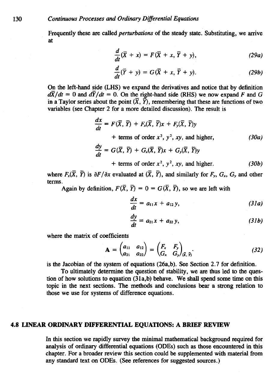
Now
consider
the
close-to-steady-state
solutions
130
Continuous Processes
and
Ordinary
Differential
Equations
Frequently these
are
called perturbations
of the
steady state. Substituting,
we
arrive
at
4.8
LINEAR ORDINARY DIFFERENTIAL EQUATIONS:
A
BRIEF REVIEW
In
this section
we
rapidly survey
the
minimal mathematical background required
for
analysis
of
ordinary differential equations (ODEs) such
as
those
encountered
in
this
chapter.
For a
broader review this section could
be
supplemented with material
from
any
standard text
on
ODEs. (See references
for
suggested sources.)
On the
left-hand side (LHS)
we
expand
the
derivatives
and
notice that
by
definition
dX/dt
= 0 and
dY/dt
= 0. On the right-hand
side (RHS)
we now
expand
F and G
in
a
Taylor
series
about
the
point
(X, Y),
remembering that these
are
functions
of two
variables (see Chapter
2 for a
more detailed discussion).
The
result
is
where
F
X
(X,
Y) is
dF/dx
evaluated
at (X, Y), and
similarly
for F
y
, G
x
, G
y
and
other
terms.
Again
by
definition, F(X,
Y) = 0 =
G(X,
Y), so we are
left
with
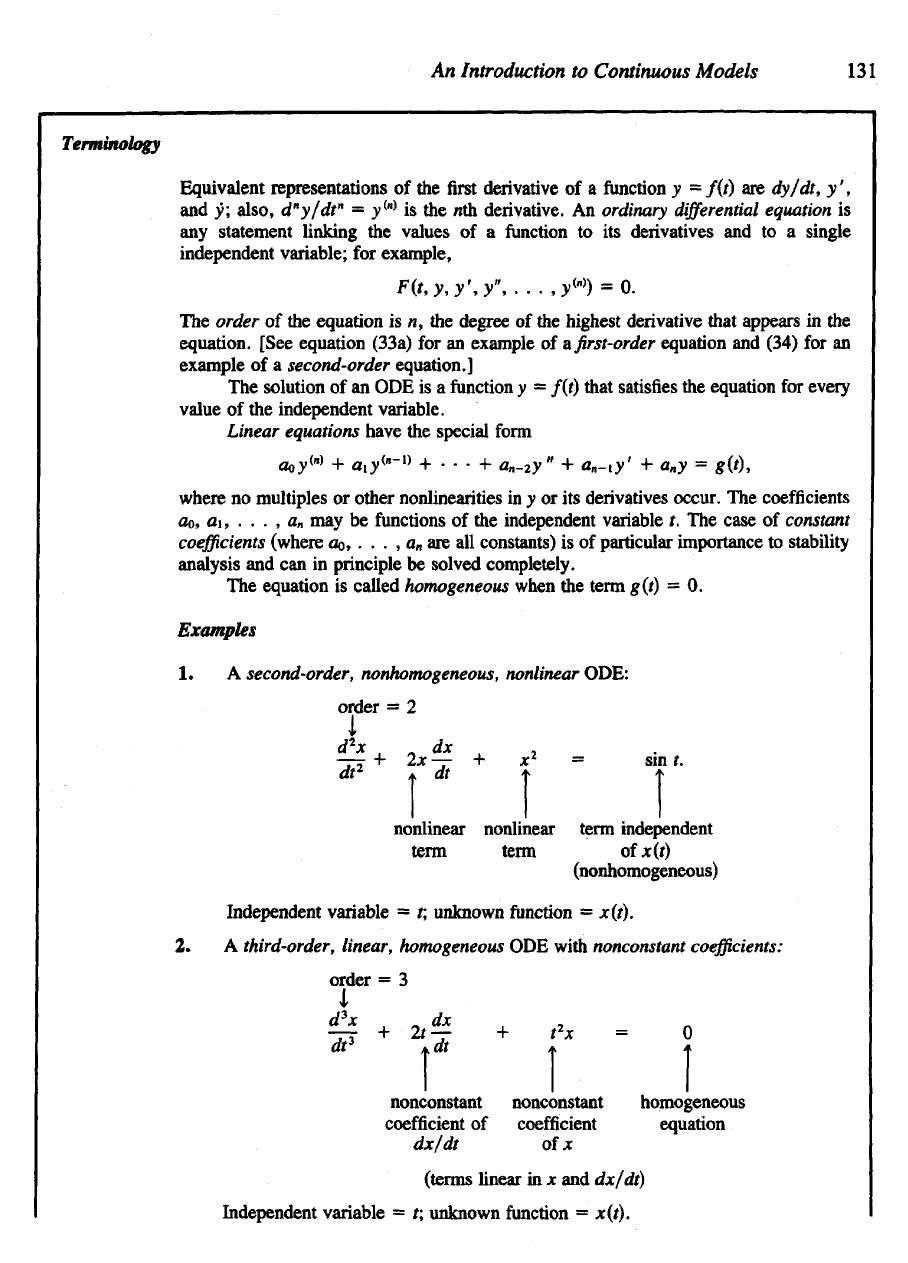
where
the
matrix
of
coefficients
is
the
Jacobian
of the
system
of
equations (26a,b).
See
Section
2.7 for
definition.
To
ultimately
determine
the
question
of
stability,
we are
thus
led to the
ques-
tion
of how
solutions
to
equation (31a,b) behave.
We
shall spend some time
on
this
topic
in the
next
sections.
The
methods
and
conclusions bear
a
strong
relation
to
those
we use for
systems
of
difference equations.
An
Introduction
to
Continuous
Models
131
Terminology
Equivalent
representations
of the first
derivative
of a
function
y =
f(i)
are
dy/dt,
y',
and
y;
also,
d
n
y/dt"
=
y
(n)
is the nth
derivative.
An
ordinary
differential
equation
is
any
statement linking
the
values
of a
function
to its
derivatives
and to a
single
independent variable;
for
example,
Independent variable
= t;
unknown function
=
*(/).
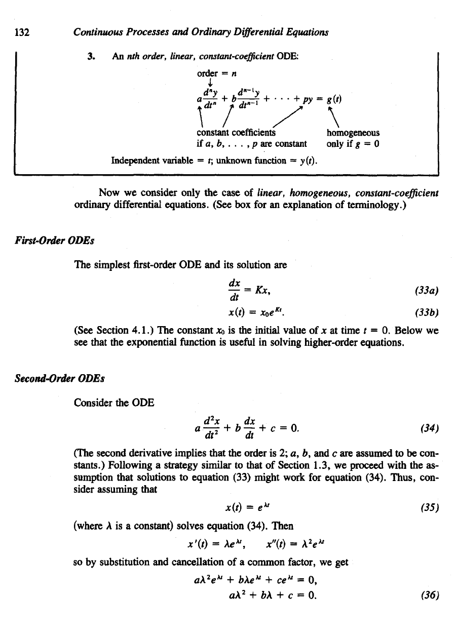
2. A
third-order, linear, homogeneous
ODE
with nonconstant
coefficients:
Independent variable
= t;
unknown
function
=
x(t).
The
order
of the
equation
is K, the
degree
of the
highest derivative that appears
in the
equation.
[See equation (33a)
for an
example
of a. first-order
equation
and
(34)
for an
example
of a
second-order equation.]
The
solution
of an ODE is a
function
y =
f(t) that satisfies
the
equation
for
every
value
of the
independent variable.
Linear
equations have
the
special
form
where
no
multiples
or
other nonlinearities
in y or its
derivatives
occur.
The
coefficients
OQ,
a\, . . . , a
n
may be
functions
of the
independent variable
t. The
case
of
constant
coefficients
(where
OQ,
. . . , a
n
are all
constants)
is of
particular importance
to
stability
analysis
and can in
principle
be
solved completely.
The
equation
is
called homogeneous
when
the
term g(t)
= 0.
Examples
1. A
second-order, nonhomogeneous,
nonlinear
ODE:
(See Section 4.1.)
The
constant
XQ
is the
initial value
of x at
time
t = 0.
Below
we
see
that
the
exponential function
is
useful
in
solving higher-order equations.
Second-Order
ODEs
Consider
the ODE
The
simplest first-order
ODE and its
solution
are
First-Order
ODEs
132
Continuous Processes
and
Ordinary
Differential
Equations
Now
we
consider only
the
case
of
linear, homogeneous,
constant-coefficient
ordinary
differential
equations. (See
box for an
explanation
of
terminology.)
(The
second
derivative
implies
that
the
order
is 2; a, b, and c are
assumed
to be
con-
stants.) Following
a
strategy similar
to
that
of
Section 1.3,
we
proceed with
the as-
sumption that
solutions
to
equation (33) might work
for
equation (34). Thus, con-
sider assuming that
so by
substitution
and
cancellation
of a
common factor,
we get
(where
A is a
constant) solves equation (34). Then
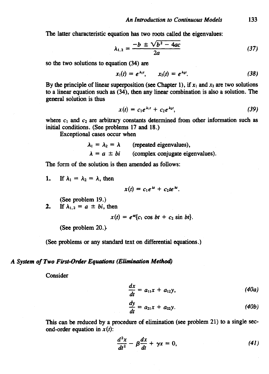
3. An nth
order, linear,
constant-coefficient
ODE:
An
Introduction
to
Continuous
Models
133
The
latter characteristic equation
has two
roots
called
the
eigenvalues:
so the two
solutions
to
equation (34)
are
By
the
principle
of
linear superposition (see Chapter
1), if x\ and x
2
are two
solutions
to a
linear equation such
as
(34), then
any
linear combination
is
also
a
solution.
The
general solution
is
thus
where
c\ and c
2
are
arbitrary constants determined
from
other information such
as
initial conditions. (See problems
17 and
18.)
Exceptional cases occur when
The
form
of the
solution
is
then amended
as
follows:
(See problems
or any
standard text
on
differential
equations.)
A
System
of Two
First-Order
Equations
(Elimination
Method)
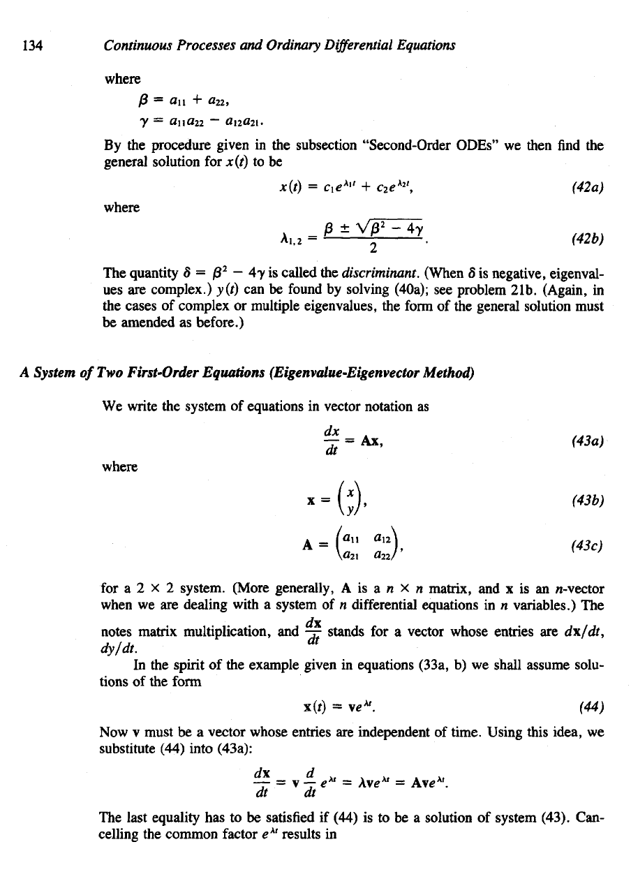
Consider
This
can be
reduced
by a
procedure
of
elimination (see problem
21) to a
single sec-
ond-order equation
in
x(i):
134
Continuous Processes
and
Ordinary
Differential
Equations
where
The
quantity
8 = /3
2
–
4-yis
called
the
discriminant. (When
8 is
negative, eigenval-
ues are
complex.) y(t)
can be
found
by
solving (40a);
see
problem 21b. (Again,
in
the
cases
of
complex
or
multiple eigenvalues,
the
form
of the
general solution must
be
amended
as
before.)
A
System
of Two
First-Order Equations (Eigenvalue-Eigenvector
Method)
We
write
the
system
of
equations
in
vector notation
as
for
a 2 x 2
system. (More generally,
A is a n x n
matrix,
and x is an
n-vector
when
we are
dealing with
a
system
of n
differential equations
in n
variables.)
The
notes matrix
multiplication,
and -r-
stands
for a
vector whose
entries
are
dx/dt,
dy/dt.
dt
In
the
spirit
of the
example given
in
equations (33a,
b) we
shall assume solu-
tions
of the
form
No
ust
be a
vector
whose entries
are
independent
of
time. Using this
idea,
we
substitute
(44) into
(43a):
The
last equality
has to be
satisfied
if
(44)
is to be a
solution
of
system (43). Can-
celling
the
common factor
e
xt
results
in
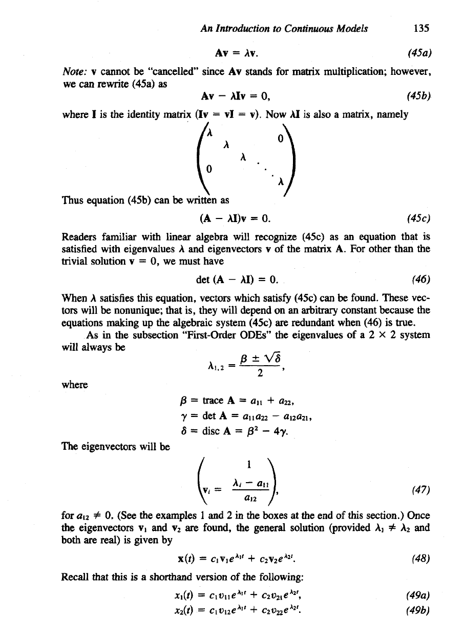
By
the
procedure given
in the
subsection "Second-Order ODEs"
we
then
find the
general solution
for
x(t)
to be
where
where
An
Introduction
to
Continuous
Models
135
Note:
v
cannot
be
"cancelled"
since
Av
stands
for
matrix multiplication; however,
we
can
rewrite (45a)
as
where
I is the
identity matrix
(Iv = vl = v). Now AI is
also
a
matrix, namely
Thus equation (45b)
can be
written
as
Readers familiar with linear algebra will recognize (45c)
as an
equation that
is
satisfied
with eigenvalues
A and
eigenvectors
v of the
matrix
A. For
other than
the
trivial
solution
v = 0, we
must have
When
A
satisfies this equation, vectors which
satisfy
(45c)
can be
found.
These vec-
tors will
be
nonunique; that
is,
they will depend
on an
arbitrary constant because
the
equations
making
up the
algebraic system (45c)
are
redundant
when
(46)
is
true.
As
in the
subsection
"First-Order
ODEs"
the
eigenvalues
of a 2 X 2
system
will always
be
where
The
eigenvectors will
be
for
a\2 =£ 0,
(See
the
examples
1 and 2 in the
boxes
at the end of
this
section.)
Once
the
eigenvectors
YI and v
2
are
found,
the
general solution (provided
Ai
i=-
Aa and
both
are
real)
is
given
by
Recall that this
is a
shorthand version
of the
following:
