Drake G.W.F. (editor) Handbook of Atomic, Molecular, and Optical Physics

Подождите немного. Документ загружается.

607

Infrared Spect

40. Infrared Spectroscopy

Infrared spectroscopy consists of the measurement

of interactions of waves of the infrared (IR)part

of the electromagnetic spectrum with matter.

The IR spectrum starts just beyond the red

part of the visible spectrum at a wavelength

λ = 700 nm and extends to the microwave region

at λ = 0.1 cm. Electromagnetic waves are generally

described in terms of their frequency ν in Hz. In

IR spectroscopy it is common practice however

to use the spatial frequency σ = ν/c.Theseare

called wavenumbers and have units of cm

−1

In this way the near, mid and far IR spectrum

spans the frequencies from 14 300 cm

−1

to 10 cm

−1

The interactions observed in the IR spectrum

involve principally the energies associated

with molecular structure change. Infrared

spectroscopy is therefore useful for molecular

structure elucidation and the identiﬁcation and

quantiﬁcation of different molecular species in

asample[40.1].

The most common IR analysis of a sample

is by IR absorption spectroscopy. This involves

transmitting a beam of intense IR radiation

through the sample and observing the

distribution of wavenumbers absorbed by the

molecules. Molecules in a sample may also be

studied by IR emission spectroscopy simply by

observing speciﬁc wavenumbers being emitted

40.1 Intensities of Infrared Radiation........... 607

40.2 Sources for IR Absorption Spectroscopy .. 608

40.3 Source, Spectrometer, Sample

and Detector Relationship .................... 608

40.4 Simpliﬁed Principle of FTIR

Spectroscopy ....................................... 608

40.4.1 Interferogram Generation:

The Michelson Interferometer ..... 609

40.4.2 Description of Wavefront

Interference with Time Delay ...... 609

40.4.3 The Operation of Spectrum

Determination .......................... 610

40.5 Optical Aspects of FTIR Technology ........ 611

40.6 The Scanning Michelson

Interferometer .................................... 612

40.7 Recent Developments........................... 613

40.8 Conclusion .......................................... 613

References .................................................. 613

by virtue of the nonzero absolute temperature

of the sample. Finally, radiation reﬂected from

a smooth surface of a solid sample also provides

information about the molecular structure of the

material by virtue of the anomalous dispersion

associated with absorption bands.

40.1 Intensities of Infrared Radiation

For strong interactions of electromagnetic waves with

matter, the emitted and absorbed intensities are governed

by Planck’s radiation law in addition to the emissiv-

ity and absorptivity of the material. Planck’s radiation

law for thermal radiation from an ideal black body

(σ) dσ =

dσ

exp(hσ/k

T ) + 1

(40.1)

where c

is a proportionality constant. Depending on

the deﬁnition of c

, P

(σ) may represent a radiation

density per unit spectral interval



−1



in a cavity

at temperature T in ergs/cm

, or an energy ﬂux emit-

ted from a surface in W/cm

steradians. At frequencies

low compared with h/k

T , the energy distribution in-

creases with σ

and is approximately proportional to

T at a given σ . At high frequency, the energy distri-

bution falls off exponentially. In the near IR, a high

temperature is required to emit radiation. Room tem-

perature objects emit strongest in the 300 to 600 cm

−1

region, and emit negligible energy above 3000 cm

−1

Materials cooled to liquid nitrogen temperature (77 K)

Part C 40

608 Part C Molecules

only emit below 100 cm

−1

, while materials cooled

to liquid helium temperature (4.2 K) only emit be-

low 20 cm

−1

. In contrast to visible spectroscopy, IR

absorption spectroscopyis complicated by emission of

IR radiation from the sample and the surrounding

environment.

40.2 Sources for IR Absorption Spectroscopy

A silicon carbide element electrically heated to 1400 K

provides a strong continuum of IR radiation over a ma-

jorpartoftheIR spectrum. It is commonly used as

a source of radiation for IR absorption spectroscopy.

For near IR spectroscopy, a tungsten ﬁlament lamp op-

erated at 2800 K provides a strong continuum all the

way up to the visible part of the spectrum; it is not

useful below 3000 cm

−1

because of absorption by the

glass or quartz envelope. Various electrically heated ce-

ramic elements, such as the Nernst glower and high

temperature carbon rods, have been devised to serve as

IR sources.

40.3 Source, Spectrometer, Sample and Detector Relationship

Since a sample at room temperature emits IR radiation

in the mid IR, it is important to distinguish between

transmitted radiation used in the determination of its

absorption spectrum and its emission spectrum. By em-

ploying an intense IR beam, the effect of emission is

minimized. Further distinction is achieved by encoding

the IR beam before it impinges on the sample.

With classical grating or prism spectrometers, the

source radiation is chopped by means of a mechani-

cal chopper before it passes through the sample. The

IR detector is provided with a means of synchronously

decoding the chopped signal, thereby eliminating the

emitted spectrum. Often the chopper is arranged such

that it alternately switches between an empty reference

beam and the sample. The logarithm of the ratio of the

demodulated sample and reference spectra provides the

absorption spectrum directly.

In Fourier Transform infrared (FTIR) Spectroscopy,

a scanning Michelson interferometer provides the en-

coding function directly and no chopper is required. The

interferometer is commonly placed before the sample so

that it does not encode the thermally emitted radiation

of the sample. Ratio recording of a sample against an

empty beam is not common in FTIR. Instead, the ab-

sorption spectrum is obtained by sequentially recording

the spectra of the sample and of the empty beam (sam-

ple removed), and computing the logarithm of the ratio

numerically.

If it is not convenient to place the sample after the

scanning Michelson interferometer, the absorption spec-

trum of a sample placed in front of the interferometer

can be deduced by subtracting the separately recorded

emission spectrum from the combined transmission plus

emission spectrum.

Infrared emission and reﬂection spectroscopy form

the basis for remote sensing. Solid and gaseous (cloud)

objects may be identiﬁed and quantiﬁed by direct obser-

vation of their IR spectra at a distance. Gaseous clouds

reﬂect poorly, providing only transmitted or emitted IR

radiation. Their emission spectrum is contrasted directly

with the spectrum of the scene or object beyond the

cloud. With a background at lower temperature than the

gas cloud, the gas spectrum appears in emission, while

with a warmer background the gas spectrum appears in

absorption.

Only a few solid materials transmit IR radiation

over a substantial thickness. Remote sensing of solid

objects relates therefore to surface emission and (dif-

fuse) reﬂection of IR radiation from the surrounding

environment.

40.4 Simpliﬁed Principle of FTIR Spectroscopy

In FTIR spectroscopy, the spectrum of a beam of in-

cident IR radiation is obtained by ﬁrst generating and

recording an interferogram with a scanning Michel-

son interferometer. Subsequently the interferogram is

inverted by means of a cosine Fourier transform into the

spectrum.

Part C 40.4

Infrared Spectroscopy 40.4 Simpliﬁed Principle of FTIR Spectroscopy 609

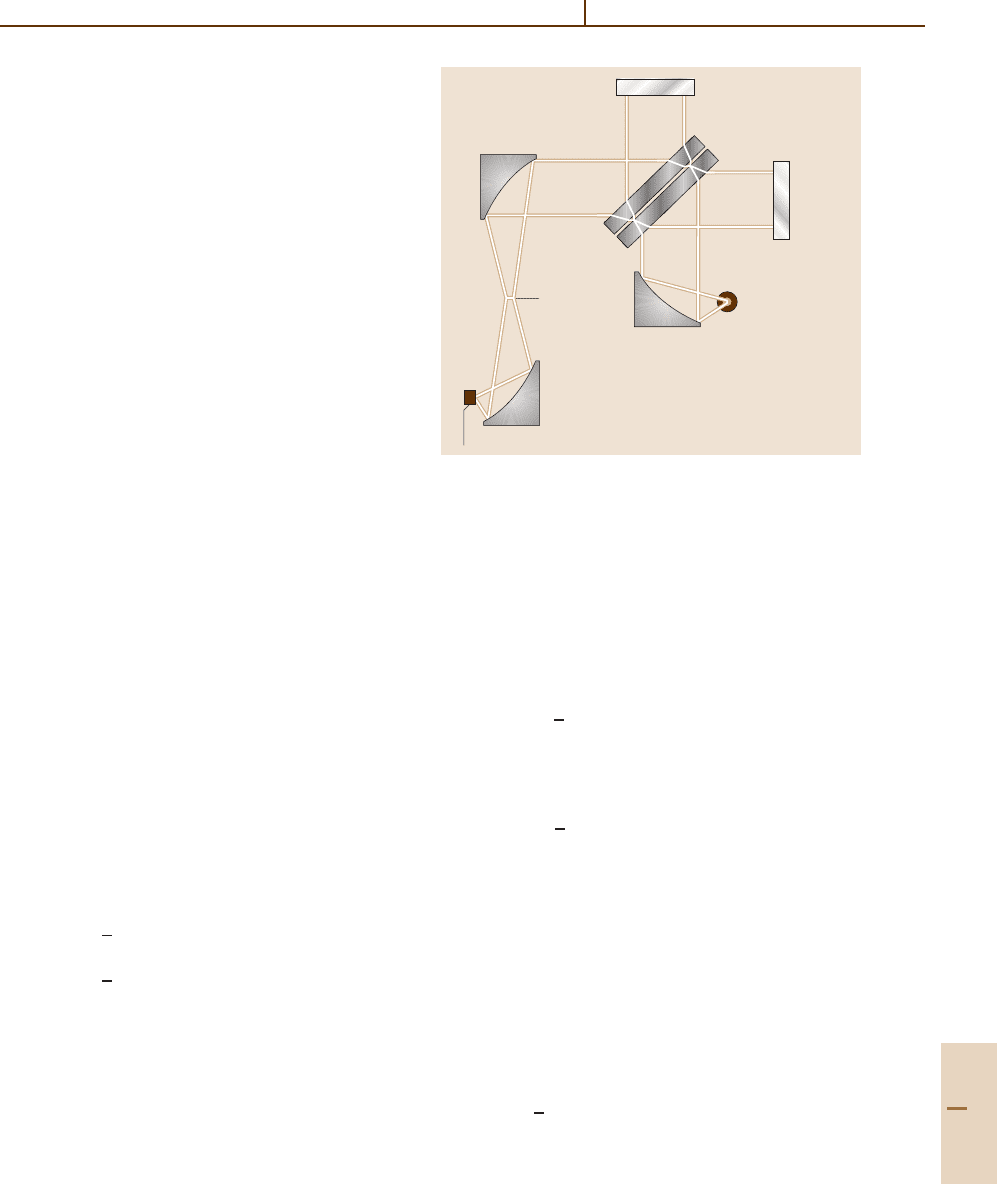
40.4.1 Interferogram Generation:

The Michelson Interferometer

The scanning Michelson interferometer shown in

Fig. 40.1 consists of a beam splitter, which is a sub-

strate with a dielectric coating such that 50% of an

incident beam is reﬂected and the remaining 50% is

transmitted, and two plane mirrors (M

and M

), one

or both of which are translated along the direction of

the beam. After splitting, the two equal amplitude wave

fronts are propagated along different optical paths. The

mirrors at the end of each path return the wavefronts

to the beamsplitter, which then acts as a wavefront

combiner. Because of their common coherent origin,

the wavefronts interfere with one another when they

combine. The state of interference is varied by scan-

ning one or both of the mirrors such that there is

a variable time delay between the two separated beams.

The resulting intensity variation of the combined out-

put beam as a function of relative time delay is the

interferogram.

40.4.2 Description of Wavefront

Interference with Time Delay

The intensity I

(ν) at frequency ν of a plane wave in

space is given by the expectation value of its elec-

tric ﬁeld vector E(ν, t) = E (ν) exp(i2πνt) according

(ν) =E(ν, t)|E(ν, t)=E (ν)

. (40.2)

The intensity at the output of the interferometer due

to an incident intensity I

(ν) is given by I(ν, δ),

where δ is the time delay between the two wavefronts

which have been propagated along two different paths,

and

I(ν, δ) =E(ν, t)+E(ν, t+δ)|E(ν, t)+E(ν, t + δ)

E (ν)



2 + e

−i2πνδ

+ e

i2πνδ



(ν)[1 + cos(2πνδ)] . (40.3)

As can be seen, the output intensity of a single frequency

source at the output of an ideal scanning Michelson

interferometer ﬂuctuates sinusoidally between zero and

the input intensity I

(ν) as the time delay δ between the

separated wavefronts is varied by means of scanning one

of the mirrors.

The quantity δ is related to mirror displacement x

with respect to equal distance of the mirrors from the

Fixed mirror

Compensator

Beam splitter

Moving

mirror

Source

Collimator

Detector

Sample

focus

Fig. 40.1 The Michelson interferometer

beamsplitter by

δ = 2x cos θ/c ,

(40.4)

where θ is the angle between the wavefront and the

optical axis of the spectrometer, and the optical axis is

the normal to each plane mirror M

and M

.Fromthis,

(40.3) becomes

(ν, x) =

(ν){1 + cos[2πν(2x cos θ/c)]} ,

(40.5)

or, using σ = ν/c,

(σ, x) =

(σ){1 + cos[2πσ(2x cos θ)]} . (40.6)

Thus the output intensity ﬂuctuates at frequency σ



2σ cos θ as a function of the mirror displacement x.

The incident intensity generally consists of a distri-

bution of intensities over many frequencies S(ν) dν with

integrated intensity



S(ν) dν. (40.7)

For this case, the output intensity of an ideal scanning

Michelson interferometer is given by

(δ) =



S(ν)[1 + cos(2πνδ)] dν.

(40.8)

The second term on the right side of (40.8)hasthe

form of the cosine Fourier transform of the spectrum.

Part C 40.4

610 Part C Molecules

By rearrangement of (40.8), it is given by



S(ν) cos(2πνδ) dν = 2I

(δ) − I

. (40.9)

The constant term I

provides no useful information

about the spectrum. The inverse cosine Fourier trans-

form of 2I

(δ) results in the spectrum S(ν) according

S(ν) =



(δ) cos(2πνδ) dδ, (40.10)

S(σ) =



(x) cos



2πσ





dx . (40.11)

Contrary to classical spectrometers, where the spec-

trum is sequentially scanned, there is no segregation of

frequencies of the input intensity. All frequencies in the

source are modulated simultaneously by the scanning

Michelson interferometer into a single interferogram

signal. This multiplex mode of spectrum determination

was ﬁrst exploited by Felgett [40.2]. It contributes to

a large advantage in sensitivity compared with other

spectrometers, and is referred to as the Felgett or multi-

plex advantage.

40.4.3 The Operation of Spectrum

Determination

The output interferogram is detected by an IR detector

which converts the intensity variations I

(x) as a func-

tion of different mirror positions x into an electrical

signal. Continuous determination of the inverse cosine

Fourier transform of the evolving interferogram re-

quires continuous multiplication of the signal by cosine

functions with all the different frequencies of the spec-

trum and integrating these products. Continuous Fourier

analysis with a bank of narrow band ﬁlters has been

implemented both in analog and digital form in early

versions of FTIRs [40.3].

It is, however, far more practical to capture the in-

terferogram signal in numeric form, using an analog to

digital converter, store it in computer memory, and com-

pute the Fourier transform numerically after the mirror

displacement range has been covered.

The numerical representation of the interferogram is

determined at known intervals of mirror displacement

∆x. The computed spectrum is then determined at reg-

ular intervals of spatial frequency ∆σ by the discrete

cosine Fourier transform

S( j∆σ) =



(n∆x) cos(2π jn∆σ∆x).

(40.12)

The sampling interval ∆x of optical path difference

determines the extent of the numerically computed spec-

trum. A higher density of sampling permits a wider

spectral range to be determined, up to

max

2∆x

(40.13)

Beyond σ

max

, the spectrum repeats in reverse order,

and beyond 2σ

max

, the spectrum repeats as is. This is

called spectral aliasing, and results from the incomplete

knowledge of the full interferogram function between

the discrete numeric representation. In order to insure

that the numeric representation of the interferogram

describes the continuous function uniquely, it is im-

portant to band limit the interferogram information to

the range 0 to σ

max

by means of optical and electrical

ﬁltering.

Conversely, the higher the density of sampling

in the spectral domain, the longer the interferogram

needs to be. For a wavenumber range ∆σ , the length

max

2∆σ

(40.14)

From the orthogonality property of the discrete

cosine Fourier transform, unique linearly independent

information can occur only at spectral intervals equal

to or greater than the sampling interval. Hence the

sampling interval in the spectrum is related to the

achievable resolution. The full width at half maxi-

mum of the representation of a single frequency in

the spectrum is 1.2∆σ . This factor applies for the

case where the single cosine wave interferogram has

been abruptly truncated at the end of the mirror scan.

The lineshape function for this case is quite oscilla-

tory due to the abrupt termination of the interferogram

signal at the end of the scan. This is not always sat-

isfactory, and frequently the interferogram is modiﬁed

by a windowing or apodization function to make the

lineshape more localized and monotonic. Apodization

always results in an increase in the full width at half

maximum.

A particularly convenient and accurate way to estab-

lish the sampling intervals of the interferogram is the use

of a single frequency laser directed coaxially with the

source radiation through the scanning Michelson inter-

ferometer. The intensity of the laser at the output of the

interferometer is a highly consistent cosine wave with

one cycle per change in mirror movement of one half

wavelength of the laser light.

Part C 40.4

Infrared Spectroscopy 40.5 Optical Aspects of FTIR Technology 611

40.5 Optical Aspects of FTIR Technology

The description of wavefront interference developed

in Sect. 40.4.2 applies to interference of plane wave

fronts only. A plane wave of IR radiation is ob-

tained at the output of a collimator optics having

an IR point source at its focus. In practice a point

source has insigniﬁcant intensity. A ﬁnite size source,

which may be represented by a distribution of point

sources in the focal plane of the collimator, provides

a distribution of plane wavefronts with different an-

gles of propagation through the scanning Michelson

interferometer.

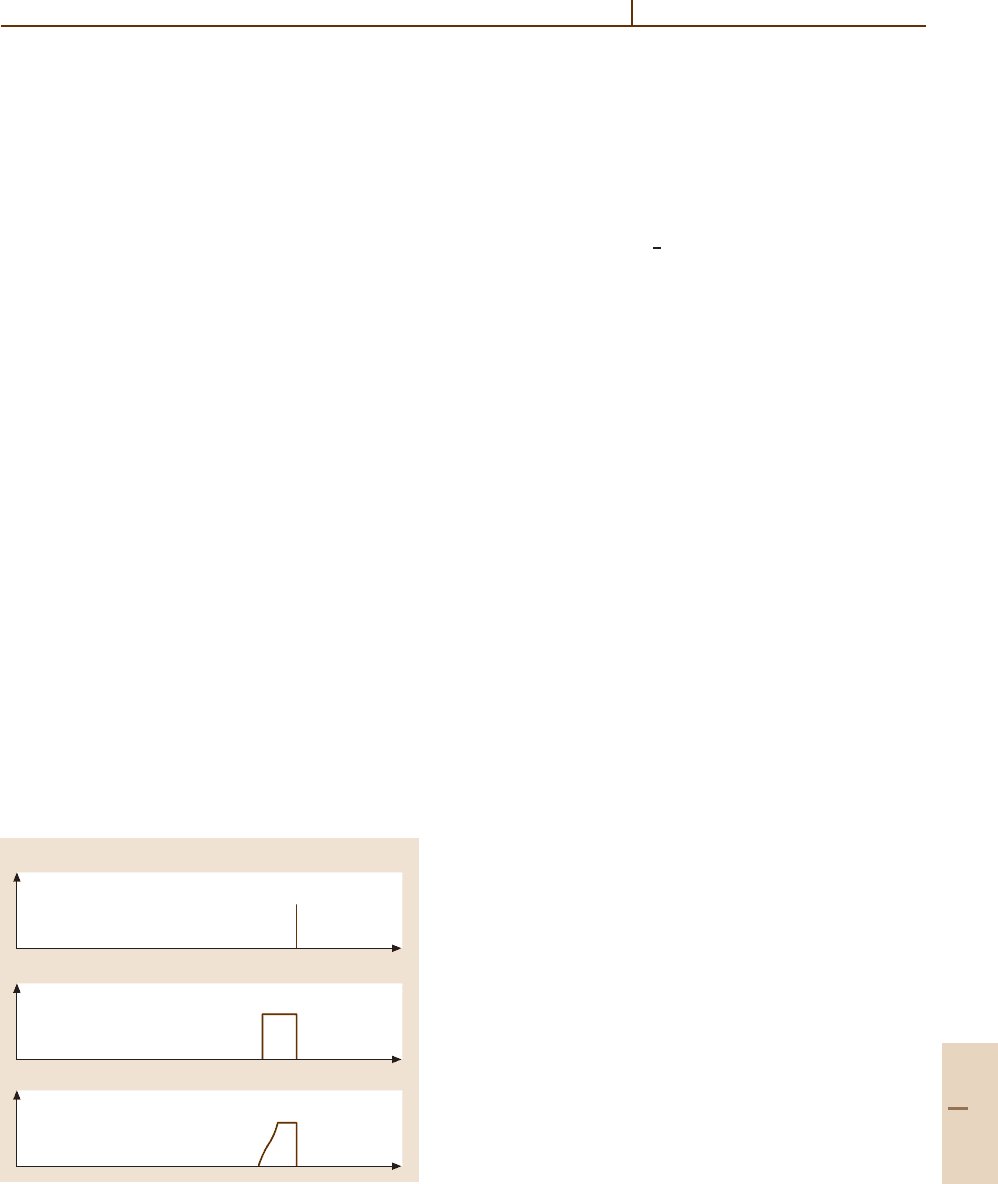
Asshownin(40.6), this distribution of angles re-

sults in a distribution of modulation frequencies as

a function of mirror displacement x of the output in-

tensity for a given IR wavenumber. This is illustrated

in Fig. 40.2 which shows, for a single frequency IR

source, the distribution of output intensity modulation

frequencies for an ideal point source on the optical axis,

a circularly symmetric distribution of uniform intensity

about the optical axis, and ﬁnally a circularly symmet-

ric distribution positioned slightly off the axis of the

collimator.

As a result of illuminating the scanning Michel-

son interferometer with a ﬁnite size source, a single

IR frequency source is observed having a distribution

of modulation frequencies in its interferogram signal.

This distribution limits the ability to resolve two closely

spaced IR frequencies and determines the optical res-

olution limit of the FTIR: The larger the extent of the

source, the more restricted the resolution becomes. The

ratio σ/∆σ is the resolving power R of the scanning

Point source on optical axis

Circular source centered on optical axis

Circular source off axis or out of focus

Michelson interferometer and, based on (40.6), is given

R = 1/(1 − cos θ

), (40.15)

where θ

is the maximum off-axis angle of illumination.

For small θ

,cosθ

≈ 1 −

,sothat

R ∼ 2/θ

. (40.16)

From (40.14), a resolution limit is also imposed by

the maximum length of the interferogram recorded.

The interferogram length dependent resolution is

constant for all spectral regions, while the optical

resolution is proportional to the spectral frequency.

Both resolution limits combine to give the over-

all resolution of an FTIR. At low resolution, the

available throughput is so high that the optical res-

olution is often negligible compared with the length

resolution. At high resolution, throughput is at a pre-

mium and the optical resolution is often closely

matched to the length resolution at the frequency of

interest.

To insure a symmetrical frequency distribution,

the area integrated illumination must increase as

sin θ, which is approximately linear for small an-

gles, up to its maximum θ

, as shown with the

centered circular illumination in Fig. 40.2. Any devi-

ation from this, such as off-axis positioning of the

circle, noncircular shapes, or a poorly focused cen-

tered symmetrical circle, will result in a gradual roll-off

of the distribution on the low frequency side only

[40.4]. This results in an asymmetric spectral line

shape.

For a collimator of given focal length and for a given

resolving power, it is easily shown that the area of the

source, or the stop that delineates it, is much larger than

the slit area for classical grating spectrometers. This is

particularly the case at high resolving powers.

This throughput advantage was ﬁrst pointed out by

Jacquinot [40.5], and plays an important role in the large

sensitivity advantage of FTIR. The stop that delineates

the source extent for a scanning Michelson interferom-

eter is often referred to as the Jacquinot stop or the ﬁeld

of view stop.

Fig. 40.2 Distribution of interferogram modulation fre-

quencies for a single optical frequency source

Part C 40.5

612 Part C Molecules

40.6 The Scanning Michelson Interferometer

Optical throughput is not only determined by the area of

the ﬁeld of view stop, but also the solid angle subtended

by the rays traversing this area. The solid angle Ω of

rays traversing a Jacquinot stop positioned in the focal

plane of an input collimator is given by the ratio of the

interferometer beam area divided by the square of the

focal length of the collimator.

For a given collimator focal length, the area of the

Jacquinot stop is inversely proportional to the resolving

power. To maintain equal throughput, the area of the

interferometer optics should be increased as resolving

power is increased in order to offset the decrease in the

Jacquinot stop area.

It is common to construct interferometers with

2.5 cm diameter optics for resolving powers up to 5000,

5.0 cm diameter optics for resolving powers up to 40 000

and 7.5 cm diameter optics for resolving powers up to

1 000 000.

In order to obtain a uniform state of interference

across the entire beam of the interferometer, the beam-

splitter substrate and the two mirrors must be ﬂat to

within a small fraction of the wavelength used. Also,

these elements must be oriented correctly so that the op-

tical path difference error across the beam is less than

a small fraction of the wavelength.

Figure 40.1 shows two substrates at the beam-

splitter position. One of the substrates supports the

beamsplitting coating, while the companion substrate

of precisely the same thickness acts as a compensat-

ing element to insure identical optical paths through

the two arms of the interferometer. To avoid sec-

ondary interference effects, both beamsplitter and

compensator substrates are normally wedged. The di-

rection of the wedges of the two substrates must be

aligned again to insure symmetry in both arms of the

interferometer.

The maintenance of a very close orientational align-

ment tolerance of the two mirrors with respect to the

beamsplitter in a stable manner over time and while

scanning one of the mirrors is the greatest challenge of

interferometer design and is also the greatest weakness

of FTIR.

In early models of FTIRs, alignment was maintained

by means of a stable mechanical structure and a highly

precise linear air bearing for the scanning mirror. Sat-

isfactory operation required a stable environment and

frequent alignment tuning and could be achieved for

mirror displacements of only several centimeters, thus

limiting the maximum resolution.

Different techniques have been developed to over-

come this weakness in FTIR. The two most prominent

are (1) Dynamic alignment of the interferometer, where

optical alignment is servo-controlled using the refer-

ence laser not only for mirror displacement control

but also for mirror orientation control, and (2) the

use of cube corner mirrors in place of the ﬂat mir-

rors in the interferometer. Dynamic alignment has the

advantage of retaining a high degree of simplicity in

the optical design of the interferometer. On the other

hand it is more complex electronically. Cube corners

have the property of always reﬂecting light 180

◦

to in-

cident light independent of orientation. Cube corners

always insure wavefront parallelism at the point of re-

combination of the two beams in the interferometer.

Cube corners lack a deﬁned optical axis. In a cube

corner interferometer, the optical axis is deﬁned as

the direction in which the wavefronts undergo zero

shear.

The scanning Michelson Interferometer is normally

provided with a drive mechanism to displace one of the

mirrors precisely parallel to its initial position and at

uniform velocity. The uniform velocity translates the

mirror displacement dependent intensities into time de-

pendent intensities. This facilitates signal processing

electronics. In some measurement scenarios however,

where the sample spectrum may vary with time, it

is undesirable to deal with the multifrequency time-

varying intensities of the interferogram signal. In this

case it is preferable to scan the moving mirror in

a stepwise mode, where the mirror is momentarily sta-

tionary at the time of signal measurement and then

advanced rapidly to the next position. The mirror scan

velocity v can be varied so that electrical signals can

have different frequencies for the same optical frequen-

cies:

f = σ/2v.

(40.17)

The scan velocity is normally selected to provide the

most favorable frequency regime for the detector and

electronics used and for the mechanical capabilities

of the mirror drive. Typically the velocity range is

from 0.05 cm/sto4cm/s, putting the frequencies in

the audio range. At these velocities, the measurement

scan may be completed in a shorter time than is de-

sired for signal averaging purposes. In this case it is

common to repeat the scan a number of times and

add the results together: this is called co-adding of

scans.

Part C 40.6

Infrared Spectroscopy References 613

40.7 Recent Developments

Added by Mark M. Cassar. Infrared spectromicroscopy,

which combines the well-established technique of

Fourier transform infrared (FTIR) spectroscopy with a

microscope, has been one of the main developments in

this area in the past decade. Recently, array detectors

have made infrared imaging practical and quick. The

brightness attainable in an IR spectromicroscope has

also been enhanced through the use of a synchrotron

radiation (SR) source, allowing the source beam to be

focused to a spot with a diameter ≤ 10 µm [40.6]. This

also allows, because of the high signal-to-noise ratio, the

measurement of dilute sample concentrations. One im-

portant application of SR-FTIR microscopy is to study

the effects of various stimuli on biomolecules in order

to understand how diseases start and spread [40.7, 8].

A testament to the robustness and versatility of

FTIR is given by its potential inclusion in future Mars

expeditions [40.9].

40.8 Conclusion

The modern technique of Fourier transform IR spec-

troscopy has evolved rapidly from its beginnings in

the early 1950s to being the dominant technique of

IR spectroscopy in many diverse disciplines. The As-

pen Conference on Fourier Spectroscopy in 1970 was

the watershed for FTIR, where many fundamental is-

sues of the technique were treated [40.10]. A practical

book by Grifﬁth and de Haseth gives many examples of

applications of FTIR [40.11].

FTIR is a powerful technique for infrared spec-

troscopy. It has a large sensitivity advantage over

conventional dispersive spectrometers because of the ef-

ﬁcient multiplexing of all the spectral elements and the

greater throughput of the Jacquinot stop. It can be used

efﬁciently for resolving powers from less than 1000 up

to 1 000 000. FTIR combines techniques of optical inter-

ferometry, laser metrology and digital signal processing.

The computation of the cosine Fourier transform

was initially a daunting task. Today, with highly

efﬁcient factoring algorithms brought to FTIR by

Forman [40.12], and the widespread availability of in-

expensive high performance personal computers, the

computation time for a Fourier transform is only

a fraction of a second per 1000 data points in the

interferogram.

A traditional weakness of FTIR is the severe

demand of alignment stability and accuracy of the

scanning Michelson interferometer. Newer optical

designs and control procedures have largely over-

come this weakness. Now FTIR can be justiﬁed

not only for its high sensitivity but also for its

high degree of reproducibility and stability, per-

mitting demanding applications in quantitative IR

analysis.

References

40.1 N. B. Colthup, L. H. Daly, S. E. Wiberley: Introduc-

tion to Infrared, Raman Spectroscopy (Academic,

New York 1990)

40.2 P. B. Fellgett: J. Phys. Radium 19, 187, 237 (1958)

40.3 J. E. Hoffman, G. A. Vanasse: J. Phys. (Paris) 28,

C2:79 (1967)

40.4 P. Saarinen, J. Kauppinnen: Appl. Opt. 31,2353

(1992)

40.5 P. Jacquinot: J. Opt. Soc. Am. 44,761(1954)

40.6 M. C. Martin: Synchrotron Radiation News 15,10

(2002)

40.7 H.-Y. N. Holman, M. C. Martin, W. McKinney:

Spectroscopy – An International Journal 17,139

(2003)

40.8 H.-Y. N. Holman, K. A. Bjornsted, M. P. McNa-

mara, M. C. Martin, W. R. McKinney, E A. Blakely:

J. Biomed. Opt. 7, 417 (2002)

40.9 M S. Anderson, J. M. Andringa, R. W. Carlson,

P. Conrad, W. Hartford, M. Shafer, A. Soto,

A. I. Tsapin, J. P. Dybwad, W. Wadsworth, K. Hand:

Rev. Sci. Instr. 76, 034101 (2005)

40.10 G. A. Vanasse, A. T. Stair, D. J. Baker (Eds.): Aspen

International Conference on Fourier Spectroscopy,

1970, AFCRL-71-0019

40.11 P. R. Grifﬁth, J. A. de Haseth: Fourier Transform In-

frared Spectrometry, J. Biomed. Opt., Vol. 83 (Wiley

Interscience, New York 1986)

40.12 M. L. Forman: J. Opt. Soc. Am. 56, 978 (1966)

Part C 40

615

Laser Spectros

41. Laser Spectroscopy in the Submillimeter

and Far-Infrared Regions

Recent technical developments in sub-millimeter

and far-infrared laser spectroscopy are described.

This includes new laser sources, both side-band

and difference-frequency generation. An exper-

iment which uses ﬁxed-frequency far-infrared

lasers to study open-shell molecules (free rad-

icals) is described; the technique is known as

laser magnetic resonance (LMR). Sub-millimeter

and far-infrared laser spectroscopies are ﬁnding

expensive use in the detection and monitoring

of molecules in astrophysical sources and in the

earth’s atmosphere.

41.1 Experimental Techniques

using Coherent SM-FIR Radiation .......... 616

41.1.1 Tunable FIR Spectroscopy

with CO

Laser Difference

Generation in a MIM Diode......... 617

41.1.2 Laser Magnetic Resonance.......... 618

41.1.3 TuFIR and LMR Detectors............. 619

41.2 Submillimeter and FIR Astronomy ......... 620

41.3 Upper Atmospheric Studies ................... 620

References .................................................. 621

Research in the submillimeter and far-infrared (SM-FIR)

regions of the electromagnetic spectrum (1000 to

150 µm, 0.3to2.0 THz; and 150 to 20 µm, 2.0

to 15 THz, respectively) had been relatively inac-

tive until about 30 years ago. Three events were

responsible for enhanced activity in this part of

the electromagnetic spectrum: the discovery of far-

infrared (FIR) lasers [41.1], the development of

background-limited detectors [41.2], and the inven-

tion of the FIR Fourier transform (FT) spectrom-

eter [41.3]. Following these developments major

discoveries have taken place in laboratory spectro-

scopic studies [41.4, 5], in astronomical observa-

tions [41.6], and in spectroscopic studies of our upper

atmosphere [41.7].

Rotational transition frequencies of light molecules

(such as hydrides) lie in this region, and the associ-

ated electric dipole transitions are especially strong at

these frequencies. In fact they are 10 000 times stronger

than at microwave frequencies because they are 100

times typical microwave frequencies and their peak

absorptivities depend approximately on the square of

the frequency. Fine structure transitions of atoms and

molecules also lie in this region; however, they are

much weaker, magnetic dipole transitions. The obser-

vation of ﬁne structure spectra is very important in

determining atomic concentrations in astronomical and

atmospheric sources and for determining the local phys-

ical conditions. Bending frequencies of larger molecules

also lie in this region, but their transitions are not as

strong as rotational transitions (typically a factor of

weaker).

Spectral accuracy has been increased by several or-

ders of magnitude with the extension of direct frequency

measurement metrology into the SM-FIR region [41.8].

Transitions whose frequencies have been measured

(including absorptions and laser emissions) are use-

ful wavelength calibration sources (λ

vac

= c/ν)for

FT spectrometers. FIR spectra of a series of rota-

tional transitions have been measured in CO [41.9],

HCl [41.10], HF [41.11], and CH

OH [41.12]tobe

used for FT calibration standards. These lines are ten

to a hundred times more accurately measured than

can be realized in present state-of-the-art Fourier trans-

form spectrometers; thus, they are excellent calibration

standards. High-accuracy and high-resolution spec-

troscopy has permitted the spectroscopic assignment of

the SM-FIR lasing transitions themselves [41.13]re-

sulting in a much better understanding of the lasing

process.

Astronomical spectroscopy in this region [41.6]may

be in emission or absorption and is performed using

either interferometric [41.14] (wavelength-based), or

heterodyne (frequency-based) [41.15] techniques to re-

solve the individual spectral features.

Most high resolution spectra of our upper atmos-

phere have been taken with FT spectrometers ﬂown

above the heavily absorbing water vapor region in the

lower atmosphere. Emission lines are generally observed

in these spectrometers [41.7].

Part C 41

616 Part C Molecules

41.1 Experimental Techniques using Coherent SM-FIR Radiation

The earliest sources of coherent SM radiation came

from harmonics of klystron radiation generated in

point-contact semiconductor diodes [41.16]. Spectro-

scopically useful powers up to about one terahertz are

produced. This technique is being replaced by electronic

oscillators which oscillate to over one terahertz [41.17].

The group at Cologne University, Germany [41.18]has

been particularly successful with this approach. Spec-

troscopy above this frequency generally is performed

with either lasers or FT spectrometers (see Chapt. 40).

Laser techniques use either tunable radiation

synthesized from the radiation of other lasers, or ﬁxed-

frequency SM-FIR laser radiation and tuning of the

transition frequency of the species by an electric or

magnetic ﬁeld. Spectroscopy with tunable far-infrared

radiation is called TuFIR spectroscopy. Spectroscopy

MIM diode

Lens

Microwave

synthesizer

(Third-order

TuFIR only)

Absorption cell

FIR

detector

Iris

FIR

Lenses

Iris

line identifier

HgCdTe

detector

Iris Lens

Iris

Lenses

AOM

laser 1

laser 2

Waveguide

laser

PZT

AOM

Reference

cells

InSb

detector

InSb

detector

Fig. 41.1 Tunable far-infrared (TuFIR) spectrometer for second- or third-order operation using CO

laser difference-

frequency generation in the MIM diode

with ﬁxed frequency lasers is called either laser electric

resonance (LER) or laser magnetic resonance (LMR).

LMR is applicable only to paramagnetic species and

is noteworthy for its extreme sensitivity. LMR spec-

troscopy has been more widely applied than LER,and

is discussed in this chapter.

Tunable SM-FIR radiation has been generated ei-

ther by adding microwave sidebands to radiation from

a SM-FIR laser [41.19]orbyusingapairofhigher

frequency lasers and generating the frequency differ-

ence [41.20]. The sideband technique was ﬁrst reported

by Dymanus [41.19] and uses a Schottky diode as

the mixing element. It has been used up to 4.25 THz

and produces a few microwatts of radiation [41.21].

Groups at Berkley, California [41.22] and Cologne, Ger-

many [41.23] have developed this technique to good

Part C 41.1

Laser Spectroscopy in the Submillimeter and Far-Infrared Regions 41.1 Experimental Techniques using Coherent SM-FIR Radiation 617

effect. The CO

laser frequency-difference technique

with difference generation in the metal-insulator-metal

(MIM) diode covers the FIR region out to over

6 THz and produces about 0.1 µW. This technique uses

ﬂuorescence-stabilized CO

lasers whose frequencies

have been directly measured, and it is about two orders of

magnitude more accurate than the sideband technique.

However, it is somewhat less sensitive because of the

decreased power available. There are several review ar-

ticles on the laser sideband technique [41.21, 24], and

only the laser difference technique is described here.

41.1.1 Tunable FIR Spectroscopy with CO

Laser Difference Generation in a MIM

Diode

There are two different ways of generating FIR radiation

using a pair of CO

lasers and the MIM diode. One is by

second-order generation, in which tunability is achieved

by using a tunable waveguide CO

laser as one of the

lasers; it is operated at about 8 kPa (60 Torr) and

is tunable by about ±120 MHz. The second technique

uses third-order generation, in which tunable microwave

sidebands are added to the difference frequency of the

two CO

lasers. The complete spectrometer which can

be operated in either second or third order is shown in

Fig. 41.1.

The FIR frequencies generated are:

second-order: ν

ﬁr



1,CO

−ν

W,CO



(41.1a)

third-order: ν

ﬁr



1,CO

−ν

W,CO



±ν

(41.1b)

where ν

ﬁr

is the tunable FIR radiation, ν

1,CO

and ν

W,CO

are the CO

laser frequencies, and ν

is the microwave

frequency.

Different MIM diodes are used for the two differ-

ent orders: in second-order, a tungsten whisker contacts

a nickel base and the normal oxide layer on nickel serves

as the insulating barrier; in third-order, a cobalt base with

its natural cobalt oxide layer is substituted for the nickel

base. The third-order cobalt diodes produce about one

third as much FIR radiation in each sideband as there is

in the second-order difference; hence third-order gener-

ation is not quite as sensitive as second-order. The much

larger tunability, however, makes it considerably easier

to use.

The common isotope of CO

is used in both the

waveguide laser and in laser 2; in laser 1, one of four iso-

topic species is used. Ninety percent of all frequencies

from 0.3to4.5 THz can be synthesized; the coverage

decreases between 4.5and6.3 THz. Ninety megahertz

acoustooptic modulators (AOMs) are used in the output

beams of the two CO

lasers which irradiate the MIM

diode; they increase the frequency coverage by an ad-

ditional 180 MHz and isolate the CO

lasers from the

MIM diode. This isolation decreases amplitude noise in

the generated FIR radiation, caused by the feedback to

the CO

laser from the MIM diode, by an order of mag-

nitude; hence, the spectrometer sensitivity increases by

an order of magnitude.

The radiations from laser 1 and the waveguide laser

are focused on the MIM diode. Laser 2 serves as a fre-

quency reference for the waveguide laser; the two lasers

beat with each other in the HgCdTe detector and a ser-

vosystem offset-locks the waveguide laser to laser 2.

Lasers 1 and 2 are frequency modulated using piezoelec-

tric drivers on the end mirrors, and they are servoed to

the line center of 4.3 µm saturated ﬂuorescence signals

obtained from the external low-pressure CO

reference

cells. In both second and third order, the CO

reference

lasers are stabilized to line center with an uncertainty

of 10 kHz. The overall uncertainty in the FIR frequency

due to two lasers is thus

√

2 × 10 or 14 kHz. This number

was determined experimentally in a measurement of the

rotational frequencies of CO out to J = 38 (4.3THz),

with the analysis of the data set determining the molecu-

lar constants [41.9].

The CO

radiation is focused by a 25 mm focal

length lens onto the conically sharpened tip of the 25 µm

diameter tungsten whisker. The FIR radiation is emitted

from the 0.1 to 3 mm long whisker in a conical long-

wire antenna pattern. Then it is collimated to a polarized

beam by a corner reﬂector [41.25] and a 30 mm focal

length off-axis segment of a parabolic mirror.

The largest uncertainty in the measurement of a tran-

sition frequency comes from ﬁnding the centers of the

Doppler broadened lines. This is about 0.05 of the line

width for lines observed with a signal-to-noise ratio of

50 or better and corresponds to about 0.05 to 0.5MHz.

A lineﬁtting program [41.26] improves the line center

determinations by nearly an order of magnitude. The FIR

radiation is frequency modulated due to a 0.5to6MHz

frequency modulation of CO

laser 1; this modulation is

at a rate of 1 kHz. The FIR detector and lock-in ampli-

ﬁer detect at this modulation rate; hence the derivatives

of the absorptions are recorded.

Absorption cells from 0.5to3.5 m in length with

diameters ranging from 19 to 30 mm have been used

in the spectrometer. The cells have either glass, copper,

or Teﬂon walls and have polyethylene or polypropylene

Part C 41.1