Drake G.W.F. (editor) Handbook of Atomic, Molecular, and Optical Physics
Подождите немного. Документ загружается.


130 Part A Mathematical Methods
This effect can be observed directly through the in-
tensity and the polarization of the light emitted from
the excited target ensemble. The perturbation coeffi-
cients for the fine structure interaction are found to
be [7.2, 13]
G(L;t)
K
=
exp(−γt)
2S+1
J
J
2J
+1
2J +1
×
LJ
S
JLK
2
cos
ω
J
−ω
J
t ,
(7.66)
where ω
J
−ω
J
corresponds to the (angular) frequency
difference between the various multiplet states with total
electronic angular momenta J
and J, respectively. Also,
γ is the natural width of the spectral line; for simplicity,
the same lifetime has been assumed in (7.66)forall
states of the multiplet.
Note that the perturbation coefficients are independ-
ent of the multipole component Q in this case, and that
there is no mixing between different multipole ranks K.
Similar results can be derived [7.2,13] for the hyperfine
interaction and also to account for the combined effect
of fine and hyperfine structure. The cosine terms repre-
sent correlation between the signal from different fine
structure states, and they lead to oscillations in the in-
tensity as well as the measured Stokes parameters in a
time-resolved experiment.
Finally, generalized perturbation coefficients have
been derived for the case where both the L and
the S systems may be oriented and/or aligned dur-
ing the collision process [7.14]. This can happen when
spin-polarized projectiles and/or target beams are pre-
pared.
7.5.3 Time Integration over Quantum Beats
If the excitation and decay times cannot be resolved in
a given experimental setup, the perturbation coefficients
need to be integrated over time. As a result, the quan-
tum beats disappear, but a net effect may still be visible
through a depolarization of the emitted radiation. For
the case of atomic fine structure interaction discussed
above, one finds [7.2, 13]
¯
G(L)
K
=
∞
0
G(L;t)
K
dt
=
1
2S+1
J
J
2J
+1
2J +1
×
LJ
S
JLK
2
γ
γ
2
+ω
2
J
J
, (7.67)
where ω
J
J
= ω
J
−ω
J
. Note that the amount of de-
polarization depends on the relationship between the
fine structure splitting and the natural line width. For
|ω
J
J
|γ (if J
= J), the terms with J
= J dominate
and cause the maximum depolarization; for the opposite
case |ω
J
J
|γ , the sum rule for the 6–j symbols can
be applied and no depolarization is observed.
Similar depolarizations can be caused through
hyperfine structure effects, as well as through external
fields. An important example of the latter case is the
Hanle effect (see Sect. 17.2.1).
7.6 Examples
In this section, two examples of the reduced den-
sity formalism are discussed explicitly. These are:
(i) the change of the spin polarization of initially
polarized spin-
1
2
projectiles after scattering from unpo-
larized targets, and (ii) the Stokes parameters describing
the angular distribution and the polarization of light
as detected in projectile-photon coincidence experi-
ments after collisional excitation. The recent book
by Andersen and Bartschat [7.4] provides a de-
tailed introduction to these topics, together with a
thorough discussion of benchmark studies in the
field of electronic and atomic collisions, including
extensions to ionization processes, as well as ap-
plications in plasma, surface, and nuclear physics.
Even more extensive compilations of such stud-
ies can be found in a review series dealing with
unpolarized electrons colliding with unpolarized tar-
gets [7.10], heavy-particle collisions [7.15], and the
special role of projectile and target spins in such col-
lisions [7.16].
7.6.1 Generalized ST U -parameters
For spin-polarized projectile scattering from unpolar-
ized targets, the generalized STU-parameters [7.11]
contain information about the projectile spin polar-
ization after the collision. These parameters can be
expressed in terms of the elements (7.36).
Part A 7.6

Density Matrices 7.6 Examples 131
To analyze this problem explicitly, one defines the
quantities
m
1
m
0
;m
1
m
0
=
1
2J
0
+1
M
1
M
0
f
M
1
m
1
; M
0
m
0
× f
∗
M
1
m
1
; M
0
m
0
(7.68)
which contain the maximum information that can be
obtained from the scattering process, if only the polar-
ization of the projectiles is prepared before the collision
and measured thereafter.
Next, the number of independent parameters that
can be determined in such an experiment needs to be ex-
amined. For spin-
1
2
particles, there are 2 × 2 × 2 × 2 =16
possible combinations of {m
1
m
0
;m
1
m
0
}and, therefore,
16 complex or 32 real parameters (in the most gen-
eral case of spin-S particles, there would be (2S+1)
4
combinations). However, from the definition (7.68)and
the Hermiticity of the reduced density matrix contained
therein, it follows that
m
1
m
0
;m
1
m
0
=
m
1
m
0
;m
1
m
0
∗
. (7.69)
Furthermore, parity conservation of the interaction or
the equivalent reflection invariance with regard to the
scattering plane yields the additional relationship [7.11]
f
M
1
m
1
; M
0
m
0
=(−1)
J
1
−M
1
+
1
2
−m
1
+J
0
−M
0
+
1
2
−m
0
× Π
1
Π
0
f
−M
1
−m
1
;−M
0
−m
0
,
(7.70)
where Π
1
and Π
0
are ±1, depending on the parities of
the atomic states involved. Hence,
m
1
m
0
;m
1
m
0
= (−1)
m
1
−m
1
+m
0
−m
0
×
−m
1
−m
0
;−m
1
−m
0
.
(7.71)
Note that (7.70, 71) hold for the collision frame where
the quantization axis (
ˆ
z) is taken as the incident beam
axis and the scattering plane is the xz-plane. Sim-
ilar formulas can be derived for the natural frame
(see Sect. 7.3.2)
Consequently, eight independent parameters are suf-
ficient to characterize the reduced spin density matrix of
the scattered projectiles. These can be chosen as the
absolute differential cross section
σ
u
=
1
2
m
1
,m
0
m
1
m
0
;m
1
m
0
(7.72)
for the scattering of unpolarized projectiles from unpo-
larized targets and the seven relative parameters
S
A
=−
2
σ
u
Im
1
2
−
1
2
;
1
2
1
2
,
(7.73)
S
P
=−
2
σ
u
Im
1
2
1
2
;−
1
2
1
2
,
(7.74)
T
y
=
1
σ
u
−
1
2
−
1
2
;
1
2
1
2
−
−
1
2
1
2
;
1
2
−
1
2
,
(7.75)
T
x
=
1
σ
u
−
1
2
−
1
2
;
1
2
1
2
+
−
1
2
1
2
;
1
2
−
1
2
,
(7.76)
T
z
=
1
σ
u
1
2
1
2
;
1
2
1
2
−
1
2
1
2
;−
1
2
1
2
,
(7.77)
U
xz
=
2
σ
u
Re
1
2
1
2
;−
1
2
1
2
,
(7.78)
U
zx
=−
2
σ
u
Re
1
2
−
1
2
;
1
2
1
2
,
(7.79)
where Re{x} and Im{x} denote the real and imaginary
parts of the complex quantity x, respectively. Note that
normalization constants have been omitted in (7.72)to
simplify the notation.
Therefore, the most general form for the polariza-
tion vector after scattering, P
, for an initial polarization
vector P = (P
x
, P
y
, P
z
) is given by
S
P
+T
y
P
y
ˆ
y +
T
x
P
x
+U
xz
P
z
ˆ
x +
T
z
P
z
−U
zx
P
x
ˆ
z
1 +S
A
P
y
.
(7.80)
The physical meaning of the above relation is illustrated
in Fig. 7.1.
The following geometries are particularly suitable
for the experimental determination of the individual par-
ameters; σ
u
and S
P
can be measured with unpolarized
incident projectiles. A transverse polarization compon-
ent perpendicular to the scattering plane
P = P
y
ˆ
y
is
needed to obtain S
A
and T
y
. Finally, the measurement of
T
x
, U
zx
, T
z
,andU
xz
requires both transverse
P
x
ˆ
x
and
longitudinal
P
z
ˆ
z
projectile polarization components in
the scattering plane.
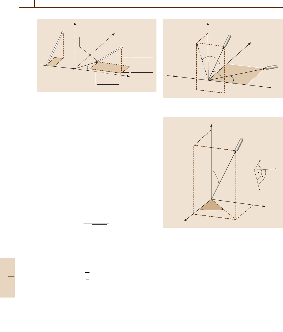
7.6.2 Radiation from Excited States:
Stokes Parameters
The state multipole description is also widely used for
the parametrization of the Stokes parameters that de-
scribe the polarization of light emitted in optical decays
of excited atomic ensembles. The general case of exci-
tation by spin-polarized projectiles has been treated by
Part A 7.6
132 Part A Mathematical Methods
P
P
z
P
y
P
x
y
x
z
P⬘
S
P
+ T
y
+ P
y
1 + S
A
+ P
y
T
x
P
x
+ U
xz
P
z
1 + S
A
P
y
T
z
P
z
– U
zx
P
z
1 + S
A
P
y
σ
u
(1 + S
A
P
y
)
k
0
k
1
θ
Fig. 7.1 Physical meaning of the generalized STU-
parameters: the polarization function S
P
gives the
polarization of an initially unpolarized projectile beam after
the collision while the asymmetry function S
A
determines
a left-right asymmetry in the differential cross section for
scattering of a spin-polarized beam. Furthermore, the con-
traction parameters (T
x
, T
y
, T
z
) describe the change of an
initial polarization component along the three cartesian axes
while the parameters U
xz
and U
zx
determine the rotation of
a polarization component in the scattering plane
Bartschat and collaborators [7.8]. The basic experimen-
tal setup for electron-photon coincidence experiments
and the definition of the Stokes parameters are illustrated
in Figs. 7.2 and 7.3.
For impact excitation of an atomic state with total
electronic angular momentum J and an electric dipole
transition to a state with J
f
, the photon intensity in
a direction
ˆ
n =(Θ
γ
,Φ
γ
) is given by
I(Θ
γ
,Φ
γ
) = C
2 (−1)
J−J
f
3
√
2J +1
T( J)
†
00
−
11 2
JJJ
f
×
Re
T( J)
†
22
sin
2
Θ
γ
cos 2Φ
γ
−Re
T( J)
†
21
sin 2Θ
γ
cos Φ
γ
+
!
1
6
T( J)
†
20
(3cos
2
Θ
γ
−1)
−Im
T( J)
†
22
sin
2
Θ
γ
sin 2Φ
γ
+ Im
T( J)
†
21
sin 2Θ
γ
sin Φ
γ
"#
,
(7.81)
where
C =
e
2
ω
4
2πc
3
$
$
J
f
rJ
$
$
2
(−1)
J−J
f
(7.82)
Θ
y
θ
e
–
, k
0
z
x
y
Φ
y
hv
e
–
, k
1
Fig. 7.2 Geometry of electron–photon coincidence experi-
ments
ˆ
n
Φ
y
z
x
y
n
Photon
detector
ˆ
e
2
ˆ
e
1
Θ
y
Fig. 7.3 Definition of the Stokes parameters: Photons are
observed in a direction
ˆ
n with polar angles (Θ
γ
,Φ
γ
) in the
collision system. The three unit vectors (
ˆ
n,
ˆ
e
1
,
ˆ
e
2
) define
the helicity system of the photons,
ˆ
e
1
= (Θ
γ
+90
◦
,Φ
γ
)
lies in the plane spanned by
ˆ
n and
ˆ
z and is perpendicular
to
ˆ
n while
ˆ
e
2
= (Θ
γ
,Φ
γ
+90
◦
) is perpendicular to both
ˆ
n and
ˆ
e
1
. In addition to the circular polarization P
3
,the
linear polarizations P
1
and P
2
are defined with respect to
axes in the plane spanned by
ˆ
e
1
and
ˆ
e
2
. Counting from the
direction of
ˆ
e
1
, the axes are located at (0
◦
, 90
◦
)forP
1
and
at (45
◦
, 135
◦
)forP
2
, respectively
is a constant containing the frequency ω of the tran-
sition as well as the reduced radial dipole matrix
element.
Similarly, the product of the intensity I and the cir-
cular light polarization P
3
can be written in terms of
Part A 7.6

Density Matrices References 133
state multipoles as
I · P
3
Θ
γ
,Φ
γ
=−C
11 1
JJJ
f
×
%
Im
T( J)
†
11
2sin Θ
γ
sinΦ
γ
−Re
T( J)
†
11
2sin Θ
γ
cosΦ
γ
+
√
2
T( J)
†
10
cos Θ
γ
&
,
(7.83)
so that P
3
can be calculated as
P
3
Θ
γ
,Φ
γ
=
I · P
3
Θ
γ
,Φ
γ
/I
Θ
γ
,Φ
γ
.
(7.84)
Note that each state multipole gives rise to a character-
istic angular dependence in the formulas for the Stokes
parameters, and that perturbation coefficients may need
to be applied to deal, for example, with depolarization
effects due to internal or external fields. General formu-
las for P
1
= η
3
and P
2
= η
1
can be found in [7.8] and,
for both the natural and the collision systems, in [7.4].
As pointed out before, some of the state multipoles
may vanish, depending on the experimental arrange-
ment. A detailed analysis of the information contained
in the state multipoles and the generalized Stokes pa-
rameters (which are defined for specific values of the
projectile spin polarization) has been given by Ander-
sen and Bartschat [7.4, 17, 18]. They re-analyzed the
experiment performed by Sohn and Hanne [7.19]and
showed how the density matrix of the excited atomic
ensemble can be determined by a measurement of the
generalized Stokes parameters. In some cases, this will
allow for the extraction of a complete set of scatter-
ing amplitudes for the collision process. Such a “perfect
scattering experiment” has been called for by Beder-
son many years ago [7.20] and is now within reach
even for fairly complex excitation processes. The most
promising cases have been discussed by Andersen and
Bartschat [7.4, 17, 21].
7.7 Summary
The basic formulas dealing with density matri-
ces in quantum mechanics, with particular empha-
sis on reduced matrix theory and its applications
in atomic physics, have been summarized. More
details are given in the introductory textbooks
by Blum [7.2], Balashov et al. [7.3], Andersen
and Bartschat [7.4], and the references listed be-
low.
References
7.1 J. von Neumann: Göttinger Nachr. 245 (1927)
7.2 K. Blum: Density Matrix Theory and Applications
(Plenum, New York 1981)
7.3 V. V. Balashov, A. N. Grum–Grzhimailo, N. M. Kabach-
nik: Polarization and Correlation Phenomena in
Atomic Collisions. A Practical Theory Course (Plenum,
New York 2000)
7.4 N. Andersen, K. Bartschat: Polarization, Alignment,
and Orientation in Atomic Collisions (Springer, New
York 2001)
7.5 J. Kessler: Polarized Electrons (Springer, New York
1985)
7.6 W. E. Baylis, J. Bonenfant, J. Derbyshire, J. Huschilt:
Am.J.Phys.61, 534 (1993)
7.7 M. Born, E. Wolf: Principles of Optics (Pergamon, New
York 1970)
7.8 K. Bartschat, K. Blum, G. F. Hanne, J. Kessler: J. Phys.
B 14, 3761 (1981)
7.9 K. Bartschat, K. Blum: Z. Phys. A 304, 85 (1982)
7.10 N. Andersen, J. W. Gallagher, I. V. Hertel: Phys. Rep.
165, 1 (1988)
7.11 K. Bartschat: Phys. Rep. 180, 1 (1989)
7.12 A. R. Edmonds: Angular Momentum in Quantum
Mechanics (Princeton Univ. Press, Princeton 1957)
7.13 U.Fano,J.H.Macek:Rev.Mod.Phys.45, 553 (1973)
7.14 K. Bartschat, H. J. Andrä, K. Blum: Z. Phys. A 314,257
(1983)
7.15 N. Andersen, J. T. Broad, E. E. Campbell, J. W. Gal-
lagher, I. V. Hertel: Phys. Rep. 278, 107 (1997)
7.16 N. Andersen, K. Bartschat, J. T. Broad, I. V. Hertel:
Phys. Rep. 279, 251 (1997)
7.17 N. Andersen, K. Bartschat: Adv. At. Mol. Phys. 36,1
(1996)
7.18 N. Andersen, K. Bartschat: J. Phys. B 27, 3189 (1994);
corrigendum: J. Phys. B 29, 1149 (1996)
7.19 M. Sohn, G. F. Hanne: J. Phys. B 25, 4627 (1992)
7.20 B. Bederson: Comments At. Mol. Phys. 1, 41,65 (1969)
7.21 N. Andersen, K. Bartschat: J. Phys. B 30, 5071 (1997)
Part A 7

135
Computationa
8. Computational Techniques
Essential to all fields of physics is the ability to
perform numerical computations accurately and
efficiently. Whether the specific approach involves
perturbation theory, close coupling expansion,
solution of classical equations of motion, or fit-
ting and smoothing of data, basic computational
techniques such as integration, differentiation, in-
terpolation, matrix and eigenvalue manipulation,
Monte Carlo sampling, and solution of differen-
tial equations must be among the standard tool
kit.
This chapter outlines a portion of this tool
kit with the aim of giving guidance and or-
ganization to a wide array of computational
techniques. Having digested the present
overview, the reader is then referred to de-
tailed treatments given in many of the large
number of texts existing on numerical anal-
ysis and computational techniques [8.1–5],
and mathematical physics [8.6–10]. We
also summarize, especially in the sections
on differential equations and computa-
tional linear algebra, the role of software
8.1 Representation of Functions................. 135
8.1.1 Interpolation ............................ 135
8.1.2 Fitting ..................................... 137
8.1.3 Fourier Analysis ........................ 139
8.1.4 Approximating Integrals ............ 139
8.1.5 Approximating Derivatives ......... 140
8.2 Differential and Integral Equations ....... 141
8.2.1 Ordinary Differential Equations ... 141
8.2.2 Differencing Algorithms
for Partial Differential Equations . 143
8.2.3 Variational Methods .................. 144
8.2.4 Finite Elements ......................... 144
8.2.5 Integral Equations..................... 146
8.3 Computational Linear Algebra .............. 148
8.4 Monte Carlo Methods ........................... 149
8.4.1 Random Numbers ..................... 149
8.4.2 Distributions of Random Numbers 150
8.4.3 Monte Carlo Integration ............. 151
References .................................................. 151
packages readily available to aid in implementing
practical solutions.
8.1 Representation of Functions
The ability to represent functions in terms of polynomi-
als or other basic functions is the key to interpolating
or fitting data, and to approximating numerically the
operations of integration and differentiation. In addi-
tion, using methods such as Fourier analysis, knowledge
of the properties of functions beyond even their inter-
mediate values, derivatives, and antiderivatives may be
determined (e.g., the “spectral” properties).
8.1.1 Interpolation
Given the value of a function f(x) at a set of points
x
1
, x
2
,... ,x
n
, the function is often required at some
other values between these abscissae. The process
known as interpolation seeks to estimate these un-
known values by adjusting the parameters of a known
function to approximate the local or global behav-
ior of f(x). One of the most useful representations
of a function for these purposes utilizes the algebraic
polynomials, P
n
(x) = a
0
+a
1
x +···+a
n
x
n
,wherethe
coefficients are real constants and the exponents are
nonnegative integers. The utility stems from the fact
that given any continuous function defined on a closed
interval, there exists an algebraic polynomial which
is as close to that function as desired (Weierstrass
Theorem).
One simple application of these polynomials is the
power series expansion of the function f(x) about some
point, x
0
,i.e.,
f(x) =
∞
k=0
a
k
(x −x
0
)
k
. (8.1)
Part A 8

136 Part A Mathematical Methods
A familiar example is the Taylor expansion in which the
coefficients are given by
a
k
=
f
(k)
(x
0
)
k !
,
(8.2)
where f
(k)
indicates the kth derivative of the function.
This form, though quite useful in the derivation of formal
techniques, is not very useful for interpolation since it
assumes the function and its derivatives are known, and
since it is guaranteed to be a good approximation only
very near the point x
0
about which the expansion has
been made.
Lagrange Interpolation
The polynomial of degree n −1 which passes through
all n points [x
1
, f(x
1
)], [x
2
, f(x
2
)],... ,[x
n
, f(x
n
)] is
given by
P(x) =
n
k=1
f(x
k
)
n
i=1,i=k
x −x
i
x
k
−x
i
(8.3)
=
n
k=1
f(x
k
)L
nk
(x), (8.4)
where L
nk
(x) are the Lagrange interpolating polynomi-
als. Perhaps the most familiar example is that of linear
interpolation between the points [x
1
, y
1
≡ f(x
1
)] and
[x
2
, y
2
≡ f(x
2
)], namely,
P(x) =
x −x
2
x
1
−x
2
y
1
+
x −x
1
x
2
−x
1
y
2
. (8.5)
In practice, it is difficult to estimate the formal error
bound for this method, since it depends on knowledge
of the (n +1)th derivative. Alternatively, one uses iter-
ated interpolation in which successively higher order
approximations are tried until appropriate agreement is
obtained. Neville’s algorithm defines a recursive pro-
cedure to yield an arbitrary order interpolant from
polynomials of lower order. This method, and subtle re-
finements of it, form the basis for most “recommended”
polynomial interpolation schemes [8.3].
One important caution to bear in mind is that the
more points that are used in constructing the inter-
polant, and therefore the higher the polynomial order,
the greater will be the oscillation in the interpolating
function. This highly oscillating polynomial most likely
will not correspond more closely to the desired function
than polynomials of lower order, and, as a general rule
of thumb, fewer than six points should be used.
Cubic Splines
By dividing the interval of interest into a number of
subintervals and in each using a polynomial of only
modest order, one may avoid the oscillatory nature of
high-order (many-point) interpolants. This approach uti-
lizes piecewise polynomial functions, the simplest of
which is just a linear segment. However, such a straight
line approximation has a discontinuous derivative at the
data points – a property that one may wish to avoid
especially if the derivative of the function is also de-
sired – and which clearly does not provide a smooth
interpolant. The solution is therefore to choose the poly-
nomial of lowest order that has enough free parameters
(the constants a
0
, a
1
,...) to satisfy the constraints that
the function and its derivative are continuous across the
subintervals, as well as specifying the derivative at the
endpoints x
0
and x
n
.
Piecewise cubic polynomials satisfy these con-
straints, and have a continuous second derivative as
well. Cubic splineinterpolation does not, however, guar-
antee that the derivatives of the interpolant agree with
those of the function at the data points, much less glob-
ally. The cubic polynomial in each interval has four
undertermined coeffitients,
P
i
(x ) =a
i
+b
i
(x −x
i
) +c
i
(x −x
i
)
2
+d
i
(x −x
i
)
3
(8.6)
for i = 0, 1,... ,n−1. Applying the constraints, a sys-
tem of equations is found which may be solved once the
endpoint derivatives are specified. If the second deriva-
tives at the endpoints are set to zero, then the result is
termed a natural spline and its shape is like that which
a long flexible rod would take if forced to pass through
all the data points. A clamped spline results if the first
derivatives are specified at the endpoints, and is usually
a better approximation since it incorporates more infor-
mation about the function (if one has a reasonable way
to determine or approximate these first derivatives).
The set of equations in the unknowns, along with
the boundary conditions, constitute a tridiagonal sys-
tem or matrix, and is therefore amenable to solution by
algorithms designed for speed and efficiency for such
systems (see Sect. 8.3;[8.1–3]). Other alternatives of
potentially significant utility are schemes based on the
use of rational functions and orthogonal polynomials.
Rational Function Interpolation
If the function which one seeks to interpolate has one or
more poles for real x, then polynomial approximations
are not good, and a better method is to use quotients of
polynomials, so-called rational functions.Thisoccurs
Part A 8.1

Computational Techniques 8.1 Representation of Functions 137
since the inverse powers of the dependent variable will
fit the region near the pole better if the order is large
enough. In fact, if the function is free of poles on the
real axis but its analytic continuation in the complex
plane has poles, the polynomial approximation may also
be poor. It is this property that slows or prevents the
convergence of power series. Numerical algorithms very
similar to those used to generate iterated polynomial
interpolants exist [8.1, 3] and can be useful for functions
which are not amenable to polynomial interpolation.
Rational function interpolation is related to the method
of Padé approximation used to improve convergence of
power series, and which is a rational function analog of
Taylor expansion.
Orthogonal Function Interpolation
Interpolation using functions other than the algebraic
polynomials can be defined and are often useful.
Particularly worthy of mention are schemes based
on orthogonal polynomials since they play a cen-
tral role in numerical quadrature. A set of functions
φ
1
(x), φ
2
(x),... ,φ
n
(x) defined on the interval [a, b]is
said to be orthogonal with respect to a weight function
W (x) if the inner product defined by
φ
i
|φ
j
=
b
a
φ
i
(x)φ
j
(x)W (x) dx (8.7)
is zero for i = j and positive for i = j. In this case, for
any polynomial P(x) of degree at most n, there exists
unique constants α
k
such that
P(x) =
n
k=0
α
k
φ
k
(x). (8.8)
Among the more commonly used orthogonal polynomi-
als are Legendre, Laguerre,andChebyshevpolynomials.
Chebyshev Interpolation
The significant advantages of employing a representa-
tion of a function in terms of Chebyshev polynomials,
T
k
(x) [8.4, 6] for tabulations, recurrence formulas, or-
thogonality properties, etc. of these polynomials), i. e.,
f(x) =
∞
k=0
a
k
T
k
(x), (8.9)
stems from the fact that (i) the expansion rapidly con-
verges, (ii) the polynomials have a simple form, and (iii)
the polynomial approximates very closely the solution
of the minimax problem. This latter property refers to the
requirement that the expansion minimizes the maximum
magnitude of the error of the approximation. In partic-
ular, the Chebyshev series expansion can be truncated
so that for a given n it yields the most accurate approx-
imation to the function. Thus, Chebyshev polynomial
interpolation is essentially as “good” as one can hope to
do. Since these polynomials are defined on the interval
[−1, 1], if the endpoints of the interval in question are a
and b, the change of variable
y =
x −
1
2
(b+a)
1
2
(b−a)
(8.10)
will effect the proper transformation. Press et al. [8.3],
for example, give convenient and efficient routines for
computing the Chebyshev expansion of a function.
8.1.2 Fitting
Fitting of data stands in distinction from interpolation
in that the data may have some uncertainty, and there-
fore, simply determining a polynomial which passes
through the points may not yield the best approximation
of the underlying function. In fitting, one is concerned
with minimizing the deviations of some model function
from the data points in an optimal or best fit manner.
For example, given a set of data points, even a low-
order interpolating polynomial might have significant
oscillation, when, in fact, if one accounts for the sta-
tistical uncertainties in the data, the best fit may be
obtained simply by considering the points to lie on
a line.
In addition, most of the traditional methods of
assigning this quality of best fit to a particular set
of parameters of the model function rely on the as-
sumption that the random deviations are described by
a Gaussian (normal) distribution. Results of physical
measurements, for example the counting of events, is
often closer to a Poisson distribution which tends (not
necessarily uniformly) to a Gaussian in the limit of
a large number of events, or may even contain “outliers”
which lie far outside a Gaussian distribution. In these
cases, fitting methods might significantly distort the pa-
rameters of the model function in trying to force these
different distributions to the Gaussian form. Thus, the
leastsquaresand chi-squarefitting procedures discussed
below should be used with this caveat in mind. Other
techniques, often termed “robust” [8.3, 11], should be
used when the distribution is not Gaussian, or replete
with outliers.
Part A 8.1

138 Part A Mathematical Methods
Least Squares
In this common approach to fitting, we wish to
determine the m parameters a
l
of some function
f(x;a
1
, a
2
,... ,a
m
) depending in this example on one
variable, x. In particular, we seek to minimize the sum
of the squares of the deviations
n
k=1
[
y(x
k
) − f(x
k
;a
1
, a
2
,... ,a
m
)
]
2
(8.11)
by adjusting the parameters, where the y(x
k
) are the n
data points. In the simplest case, the model function is
just a straight line, f(x;a
1
, a
2
) = a
1
x +a
2
.Elementary
multivariate calculus implies that a minimum occurs if
a
1
n
k=1
x
2
i
+a
2
n
k=1
x
i
=
n
k=1
x
i
y
i
, (8.12)
a
1
n
k=1
x
i
+a
2
n =
n
k=1
y
i
, (8.13)
which are called the normal equations. Solution of these
equations is straightforward, and an error estimate of
the fit can be found [8.3]. In particular, variances may
be computed for each parameter, as well as measures
of the correlation between uncertainties and an overall
estimate of the “goodness of fit” of the data.
Chi-square Fitting
If the data points each have associated with them a dif-
ferent standard deviation, σ
k
, the least square principle
is modified by minimizing the chi-square,definedas
χ
2
≡
n
k=1
y
k
− f(x
k
;a
1
, a
2
,... ,a
m
)
σ
k
2
. (8.14)
Assuming that the uncertainties in the data points are
normally distributed, the chi-square value gives a mea-
sure of the goodness of fit. If there are n data points
and m adjustable parameters, then the probability that
χ
2
should exceed a particular value purely by chance is
Q = Q
n −m
2
,
χ
2
2
,
(8.15)
where Q(a, x) = Γ(a, x)/Γ(a) is the incomplete gamma
function. For small values of Q, the deviations of the fit
from the data are unlikely to be by chance, and values
close to one are indications of better fits. In terms of the
chi-square, reasonable fits often have χ
2
≈ n−m.
Other important applications of the chi-square
method include simulation and estimating standard de-
viations. For example, if one has some idea of the actual
(i. e., non-Gaussian) distribution of uncertainties of the
data points, Monte Carlo simulation can be used to gen-
erate a set of test data points subject to this presumed
distribution, and the fitting procedure performed on the
simulated data set. This allows one to test the accu-
racy or applicability of the model function chosen. In
other situations, if the uncertainties of the data points
are unknown, one can assume that they are all equal to
some value, say σ, fit using the chi-square procedure,
and solve for the value of σ. Thus, some measure of
the uncertainty from this statistical point of view can be
provided.
General Least Squares
The least squares procedure can be generalized usually
by allowing any linear combination of basis functions to
determine the model function
f(x;a
1
, a
2
,... ,a
m
) =
m
l=1
a
l
ψ
l
(x). (8.16)
The basis functions need not be polynomials. Similarly,
the formula for chi-square can be generalized, and nor-
mal equations determined through minimization. The
equations may be written in compact form by defining
amatrix A with elements
A
i, j
=
ψ
j
(x
i
)
σ
i
, (8.17)
and a column vector B with elements
B
i
=
y
i
σ
i
. (8.18)
Then the normal equations are [8.3]
m
j=1
α
kj
a
j
= β
k
, (8.19)
where
[α]=A
T
A, [β]=A
T
B , (8.20)
and a
j
are the adjustable parameters. These equations
may be solved using standard methods of computational
linear algebra such as Gauss–Jordan elimination. Diffi-
culties involving sensitivity to round-off errors can be
avoided by using carefully developed codes to perform
this solution [8.3]. We note that elements of the inverse
of the matrix α are related to the variances associated
with the free parameters and to the covariances relating
them.
Part A 8.1

Computational Techniques 8.1 Representation of Functions 139
Statistical Analysis of Data
Data generated by an experiment, or perhaps from
a Monte Carlo simulation, have uncertainties due to
the statistical, or random, character of the processes by
which they are acquired. Therefore, one must be able
to describe statistically certain features of the data such
as their mean, variance and skewness, and the degree
to which correlations exist, either between one portion
of the data and another, or between the data and some
other standard or model distribution. A very readable
introduction to this type analysis has been given by
Young [8.12], while more comprehensive treatments are
also available [8.13].
8.1.3 Fourier Analysis
The Fourier transform takes, for example, a function of
time, into a function of frequency, or vice versa, namely
˜
ϕ(ω) =
1
√
2π
∞
−∞
ϕ(t) e
iωt
dt , (8.21)
ϕ(t) =
1
√
2π
∞
−∞
˜
ϕ(ω) e
−iωt
dω. (8.22)
In this case, the time history of the function ϕ(t) may be
termed the “signal” and
˜
ϕ(ω) the “frequency spectrum”.
Also, if the frequency is related to the energy by E =
ω,
one obtains an “energy spectrum” from a signal, and thus
the name spectral methods for techniques based on the
Fourier analysis of signals.
The Fourier transform also defines the relationship
between the spatial and momentum representations of
wave functions, i. e.,
ψ(x) =
1
√
2π
∞
−∞
˜
ψ(p)e
i px
dp , (8.23)
˜
ψ(p) =
1
√
2π
∞
−∞
ψ(x) e
−ipx
dx . (8.24)
Along with the closely related sine, cosine,and
Laplace transforms, the Fourier transform is an extraor-
dinarily powerful tool in the representation of functions,
spectral analysis, convolution of functions, filtering, and
analysis of correlation. Good introductions to these tech-
niques with particular attention to applications in physics
can be found in [8.6, 7, 14]. To implement the Fourier
transform numerically, the integral tranform pair can be
converted to sums
˜
ϕ(ω
j
) =
1
√
2N2π
2N−1
k=0
ϕ(t
k
)e
iω
j
t
k
, (8.25)
ϕ(t
k
) =
1
√
2N2π
2N−1
j=0
˜
ϕ(ω
j
)e
−iω
j
t
k
, (8.26)
where the functions are “sampled” at 2N points. These
equations define the discrete Fourier transform (DFT).
Two cautions in using the DFT are as follows.
First, if a continuous function of time that is sam-
pled at, for simplicity, uniformly spaced intervals,
(i. e., t
i+1
= t
i
+∆), then there is a critical frequency
ω
c
= π/∆, known as the Nyquist frequency, which lim-
its the fidelity of the DFT of this function in that it
is aliased. That is, components outside the frequency
range −ω
c
to ω
c
are falsely transformed into this range
due to the finite sampling. This effect can be remedi-
ated by filtering or windowing techniques. If, however,
the function is bandwidth limited to frequencies smaller
than ω
c
, then the DFT does not suffer from this effect,
and the signal is completely determined by its samples.
Second, implementing the DFT directly from the above
equations would require approximately N
2
multiplica-
tions to perform the Fourier transform of a function
sampled at N points. A variety of fast Fourier trans-
form (FFT) algorithms have been developed (e.g., the
Danielson–Lanczos and Cooley–Tukey methods) which
require only on the order of (N/2) log
2
N multiplica-
tions. Thus, for even moderately large sets of points, the
FFT methods are indeed much faster than the direct im-
plementation of the DFT. Issues involved in sampling,
aliasing, and selection of algorithms for the FFT are
discussed in great detail, for example, in [8.3, 15, 16].
8.1.4 Approximating Integrals
Polynomial Quadrature
Definite integrals may be approximated through a pro-
cedure known as numerical quadrature by replacing the
integral by an appropriate sum, i. e.,
b
a
f(x) dx ≈
n
k=0
a
k
f(x
k
). (8.27)
Most formulas for such approximation are based on the
interpolating polynomials described in Sect. 8.1.1,es-
pecially the Lagrange polynomials, in which case the
Part A 8.1

140 Part A Mathematical Methods
coefficients a
k
are given by
a
k
=
b
a
L
nk
(x
k
)dx . (8.28)
If first or second degree Lagrange polynomials are used
with a uniform spacing between the data points, one
obtains the trapezoidal and Simpson’s rules,i.e.,
b
a
f(x) dx ≈
δ
2
[
f(a) + f(b)
]
+O
δ
3
f
(2)
(ζ)
,
(8.29)
b
a
f(x) dx ≈
δ
3
f(a) +4 f
δ
2
+ f(b)
+O
δ
5
f
(4)
(ζ)
, (8.30)
respectively, with δ =b−a, and for some ζ in [a, b].
Other commonly used formulas based on low-order
polynomials, and generally referred to as Newton–Cotes
formulas, are described and discussed in detail in numer-
ical analysis texts [8.1, 2]. Since potentially unwanted
rapid oscillations in interpolants may arise, it is gener-
ally the case that increasing the order of the quadrature
scheme too greatly does not generally improve the ac-
curacy of the approximation. Dividing the interval [a, b]
into a number of subintervals and summing the result
of application of a low-order formula in each subinter-
val is usually a much better approach. This procedure,
referred to as composite quadrature, may be combined
with choosing the data points at a nonuniform spacing,
decreasing the spacing where the function varies rapidly,
and increasing the spacing for economy where the func-
tion is smooth to construct an adaptive quadrature.
Gaussian Quadrature
If the function whose definite integral is to be ap-
proximated can be evaluated explicitly, then the data
points (abscissas) can be chosen in a manner in which
significantly greater accuracy may be obtained than us-
ing Newton–Cotes formulas of equal order. Gaussian
quadrature is a procedure in which the error in the
approximation is minimized owing to this freedom to
choose both data points (abscissas) and coefficients. By
utilizing orthogonal polynomials and choosing the ab-
scissas at the roots of the polynomials in the interval
under consideration, it can be shown that the coeffi-
cients may be optimally chosen by solving a simple set
of linear equations. Thus, a Gaussian quadrature scheme
approximates the definite integral of a function multipled
by the weight function appropriate to the orthogonal
polynomial being used as
b
a
W (x) f(x) dx ≈
n
k=1
a
k
f(x
k
), (8.31)
where the function is to be evaluated at the abscissas
given by the roots of the orthogonal polynomial, x
k
.
In this case, the coefficients a
k
are often referred to
as “weights,” but should not be confused with the
weight function W (x) (Sect. 8.1.1). Since the Legen-
dre polynomials are orthogonal over the interval [−1, 1]
with respect to the weight function W (x) ≡ 1, this
equation has a particularly simple form, leading im-
mediately to the Gauss–Legendre quadrature.If f(x)
contains as a factor the weight function of another of
the orthogonal polynomials, the corresponding Gauss–
Laguerre or Gauss–Chebyshev quadrature should be
used.
The roots and coefficients have been tabulated [8.4]
for many common choices of the orthogonal polyno-
mials (e.g., Legendre, Laguerre, Chebyshev) and for
various orders. Simple computer subroutines are also
available which conveniently compute them [8.3]. Since
the various orthogonal polynomials are defined over dif-
ferent intervals, use of the change of variables such as
that given in (8.10) may be required. So, for Gauss–
Legendre quadrature we make use of the transformation
b
a
f(x) dx ≈
(b−a)
2
1
−1
f
(b−a)y+b+a
2
dy .
(8.32)
Other Methods
Especially for multidimensional integrals which can not
be reduced analytically to seperable or iterated integrals
of lower dimension, Monte Carlo integration may pro-
vide the only means of finding a good approximation.
This method is described in Sect. 8.4.3. Also, a conve-
nient quadrature scheme can easily be devised based on
the cubic spline interpolation described in Sect. 8.1.1.
since in each subinterval, the definite integral of a cubic
polynomial of known coefficients is evident.
8.1.5 Approximating Derivatives
Numerical Differentiation
The calculation of derivatives from a numerical repre-
sentaion of a function is generally less stable than the
Part A 8.1