Dougherty С. Introduction to Econometrics, 3Ed
Подождите немного. Документ загружается.


SIMPLE REGRESSION ANALYSIS
6
T
ABLE
2.1
XY
Y
ˆ
e
13b
1
+ b
2
3 – b
1
– b
2
25b
1
+ 2b
2
5 – b
1
– 2b
2
We shall assume that the true model is
Y
i
=
β
1
+
β
2
X
i
+ u
i
(2.6)
and we shall estimate the coefficients b
1
and b
2
of the equation
ii
XbbY
21
ˆ
+=
. (2.7)
Obviously, when there are only two observations, we can obtain a perfect fit by drawing the regression
line through the two points, but we shall pretend that we have not realized this. Instead we shall arrive
at this conclusion by using the regression technique.
When X is equal to 1, Y
ˆ
is equal to (b
1
+ b
2
), according to the regression line. When X is equal to
2,
Y
ˆ
is equal to (b
1
+ 2b
2
). Therefore, we can set up Table 2.1. So the residual for the first
observation, e
1
, which is given by (Y
1
–
1
ˆ
Y ), is equal to (3 – b
1
– b
2
), and e
2
, given by (Y
2
–
2
ˆ
Y ), is
equal to (5 – b
1
– 2b
2
). Hence
2121
2
2
2
1
2121
2
2
2
1
2121
2
2
2
1
2
21
2
21
626165234
42010425
2669
)25()3(
bbbbbb
bbbbbb
bbbbbb
bbbbRSS
+−−++=
+−−+++
+−−++=
−−+−−=
(2.8)
Now we want to choose b
1
and b
2
to minimize RSS. To do this, we use the calculus and find the
values of b
1
and b
2
that satisfy
0
1
=
b
RSS
∂
∂
and
0
2
=
b
RSS
∂
∂
(2.9)
Taking partial differentials,
1664
21
1
−+=
bb
b
RSS
∂
∂
(2.10)
and
26610
12
2
−+=
bb
b
RSS
∂
∂
(2.11)
and so we have
SIMPLE REGRESSION ANALYSIS
7
2b
1
+ 3b
2
– 8 = 0 (2.12)
and
3b
1
+ 5b
2
– 13 = 0 (2.13)
Solving these two equations, we obtain b
1
= 1 and b
2
= 2, and hence the regression equation
ii
XY 21
ˆ
+=
(2.14)
Just to check that we have come to the right conclusion, we shall calculate the residuals:
e
1
= 3 – b
1
– b
2
= 3 – 1 – 2 = 0 (2.15)
e
2
= 5 – b
1
– 2b
2
= 5 – 1 – 4 = 0 (2.16)
Thus both the residuals are 0, implying that the line passes exactly through both points, which of
course we knew from the beginning.
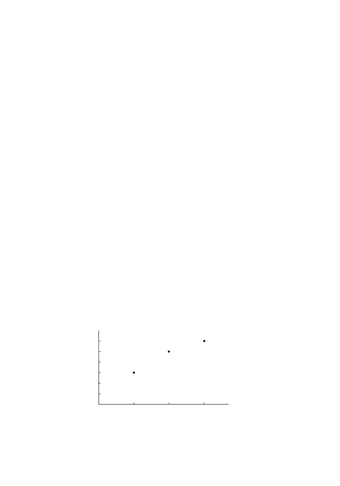
Example 2
We shall take the example in the previous section and add a third observation: Y is equal to 6 when X
is equal to 3. The three observations, shown in Figure 2.5, do not lie on a straight line, so it is
impossible to obtain a perfect fit. We will use least squares regression analysis to calculate the
position of the line.
We start with the standard equation
ii
XbbY
21
ˆ
+=
. (2.17)
For values of X equal to 1, 2, and 3, this gives fitted values of Y equal to (b
1
+ b
2
), (b
1
+ 2b
2
), and
(b
1
+ 3b
2
), respectively, and one has Table 2.2.
Figure 2.5.
Three-observation example
1
2
3
4
5
6
Y
123
X
SIMPLE REGRESSION ANALYSIS
8
T
ABLE
2.2
XY
Y
ˆ
e
13b
1
+ b
2
3 – b
1
– b
2
25b
1
+ 2b
2
5 – b
1
– 2b
2
36b
1
+ 3b
2
6 – b
1
– 3b
2
Hence
2121
2
2
2
1
2121
2
2
2
1
2121
2
2
2
1
2121
2
2
2
1
2
21
2
21
2
21
12622814370
63612936
42010425
2669
)36()25()3(
bbbbbb
bbbbbb
bbbbbb
bbbbbb
bbbbbbRSS
+−−++=
+−−+++
+−−+++
+−−++=
−−+−−+−−=
(2.18)
The first-order conditions
0
1
=
b
RSS
∂
∂
and
0
2
=
b
RSS
∂
∂
give us
6b
1
+ 12b
2
– 28 = 0 (2.19)
and
12b
1
+ 28b
2
– 62 = 0 (2.20)
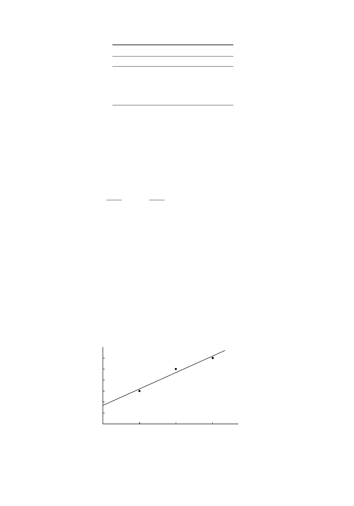
Solving these two equations, one obtains b
1
= 1.67 and b
2
= 1.50. The regression equation is therefore
ii
XY 50.167.1
ˆ
+=
(2.21)
The three points and the regression line are shown in Figure 2.6.
Figure 2.6.
Three-observation example with regression line
1
2
3
4
5
6
Y
123
X

SIMPLE REGRESSION ANALYSIS
9
2.4 Least Squares Regression with One Explanatory Variable
We shall now consider the general case where there are n observations on two variables X and Y and,
supposing Y to depend on X, we will fit the equation
ii
XbbY
21
ˆ
+=
. (2.22)
The fitted value of the dependent variable in observation i,
i
Y
ˆ
, will be (b
1
+ b
2
X
i
), and the residual e
i
will be (Y
i
– b
1
– b
2
X
i
). We wish to choose b
1
and b
2
so as to minimize the residual sum of the squares,
RSS, given by
∑
=
=++=
n
i
in
eeeRSS
1
222
1
...
(2.23)
We will find that RSS is minimized when
)Var(
),(Cov
2
X
YX
b
=
(2.24)
and
XbYb
21
−=
(2.25)
The derivation of the expressions for b
1
and b
2
will follow the same procedure as the derivation in
the two preceding examples, and you can compare the general version with the examples at each step.
We will begin by expressing the square of the residual in observation i in terms of b
1
, b
2
, and the data
on X and Y:
iiiiii
iiiii
XbbYXbYbXbbY
XbbYYYe
2121
22
2
2
1
2
2
21
22
222
)()
ˆ
(
+−−++=
−−=−=
(2.26)
Summing over all the n observations, we can write RSS as
∑∑∑∑∑
=====
+−−++=
+−−+++
+
+−−++=
−−++−−=
n
i
i
n
i
ii
n
i
i
n
i
i
n
i
i
nnnnnn
nn
XbbYXbYbXbnbY
XbbYXbYbXbbY
XbbYXbYbXbbY
XbbYXbbYRSS
1
21
1
2
1
1
1
22
2
2
1
1
2
2121
22
2
2
1
2
12111211
2
1
2
2
2
1
2
1
2
21
2
1211
222
222
...
222
)(...)(
(2.27)
Note that RSS is effectively a quadratic expression in b
1
and b
2
, with numerical coefficients
determined by the data on X and Y in the sample. We can influence the size of RSS only through our

SIMPLE REGRESSION ANALYSIS
10
choice of b
1
and b
2
. The data on X and Y, which determine the locations of the observations in the
scatter diagram, are fixed once we have taken the sample. The equation is the generalized version of
equations (2.8) and (2.18) in the two examples.
The first order conditions for a minimum,
0
1
=
b
RSS
∂
∂
and
0
2
=
b
RSS
∂
∂
, yield the following
equations:
0222
1
2
1
1
=+−
∑∑
==
n
i
i
n
i
i
XbYnb
(2.28)
0222
1
1
11
2
2
=+−
∑∑∑
===
n
i
i
n
i
ii
n
i
i
XbYXXb
(2.29)
These equations are known as the normal equations for the regression coefficients and are the
generalized versions of (2.12) and (2.13) in the first example, and (2.19) and (2.20) in the second.
Equation (2.28) allows us to write b
1
in terms of
Y
,
X
, and the as yet unknown b
2
. Noting that
∑
=
=
n
i
i
X
n
X
1
1
and
∑
=
=
n
i
i
Y
n
Y
1
1
, (2.28) may be rewritten
0222
21
=+−
XnbYnnb (2.30)
and hence
XbYb
21
−=
. (2.31)
Substituting for b
1
in (2.29), and again noting that
XnX
n
i
i
=
∑
=
1
, we obtain
0)(222
2
11
2
2
=−+−
∑∑
==
XnXbYYXXb
n
i
ii
n
i
i
(2.32)
Separating the terms involving b
2
and not involving b
2
on opposite sides of the equation, we have
YXnYXXnXb
n
i
ii
n
i
i
222
1
2
1
2
2
−=
−
∑∑
==
(2.33)
Dividing both sides by 2n,
YXYX
n
bXX
n
n
i
ii
n
i
i
−
=
−
∑∑
==
1
2
2
1
2
11
(2.34)

SIMPLE REGRESSION ANALYSIS
11
Using the alternative expressions for sample variance and covariance, this may be rewritten
b
2
Var(X) = Cov(X,Y) (2.35)
and so
)(Var
),(Cov
2
X
YX
b
=
(2.36)
Having found b
2
from (2.36), you find b
1
from (2.31). Those who know about the second order
conditions will have no difficulty confirming that we have minimized RSS.
In the second numerical example in Section 2.3, Cov(X, Y) is equal to 1.000, Var(X) to 0.667,
Y
to 4.667,
X
to 2.000, so
b
2
= 1.000/0.667 = 1.50 (2.37)
and
XbYb
21
−=
= 4.667 – 1.50
×
2.000 = 1.667, (2.38)
which confirms the original calculation.
Alternative Expressions for b
2
From the definitions of Cov(X, Y) and Var(X) one can obtain alternative expressions for b
2
in
Σ
notation:
∑
∑
∑
∑
=
=
=
=
−
−−
=
−
−−
==
n
i
i
n
i
ii
n
i
i
n
i
ii
XX
YYXX
XX
n
YYXX
n
X
YX
b
1
2
1
1
2
1
2
)(
))((
)(
1
))((
1
)(Var
),(Cov
(2.39)
One may obtain further variations using the alternative expressions for Cov(X, Y) and Var(X) provided
by equations (1.8) and (1.16):
2
1
2
1
2
1
2
1
2
1
1
XnX
YXnYX
XX
n
YXYX
n
b
n
i
i
n
i
ii
n
i
i
n
i
ii
−
−
=
−
−
=
∑
∑
∑
∑
=
=
=
=
(2.40)
SIMPLE REGRESSION ANALYSIS
12
2.5 Two Decompositions of the Dependent Variable
In the preceding pages we have encountered two ways of decomposing the value of the dependent
variable in a regression model. They are going to be used throughout the text, so it is important that
they be understood properly and that they be kept apart conceptually.
The first decomposition relates to the process by which the values of Y are generated:
Y
i
=
β
1
+
β
2
X
i
+ u
i
. (2.41)
In observation i, Y
i
is generated as the sum of two components, the nonstochastic component,
β
1
+
β
2
X
i
, and the disturbance term u
i
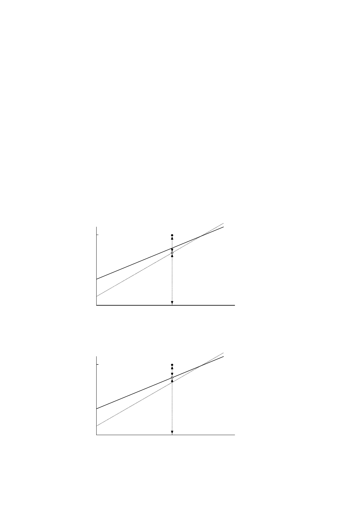
. This decomposition is purely theoretical. We will use it in the
analysis of the properties of the regression estimators. It is illustrated in Figure 2.7a, where QT is the
nonstochastic component of Y and PQ is the disturbance term
The other decomposition relates to the regression line:
ii
iii
eXbb
eYY
++=
+=
21
ˆ
. (2.42)
Figure 2.7a.
Decomposition of
Y
into nonstochastic component and disturbance term
Figure 2.7b.
Decomposition of
Y
into fitted value and residual
Y
X
u
i
β
1
+
β
2
X
i
P
b
1
β
1
X
i
Y
i
Q
T
XbbY
21
+=
ˆ
XY
21
β
β
+=
Y
X
e
i
b
1
+
b
2
X
i
b
1
β
1
X
i
Y
i
R
T
P
XY
21
β
β
+=
XbbY
21
+=
ˆ

SIMPLE REGRESSION ANALYSIS
13
Once we have chosen the values of b
1
and b
2
, each value of Y is split into the fitted value,
i
Y
ˆ
, and the
residual, e
i
. This decomposition is operational, but it is to some extent arbitrary because it depends on
our criterion for determining b
1
and b
2
and it will inevitably be affected by the particular values taken
by the disturbance term in the observations in the sample. It is illustrated in Figure 2.7b, where RT is
the fitted value and PR is the residual.
2.6 Interpretation of a Regression Equation
There are two stages in the interpretation of a regression equation. The first is to turn the equation into
words so that it can be understood by a noneconometrician. The second is to decide whether this
literal interpretation should be taken at face value or whether the relationship should be investigated
further.
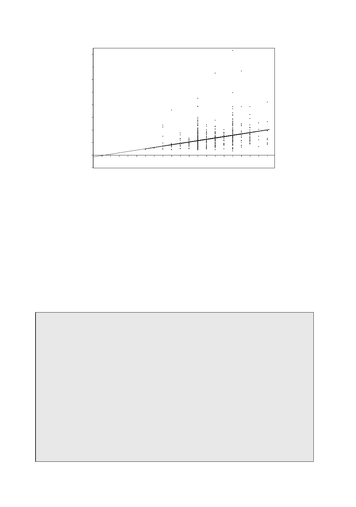
Both stages are important. We will leave the second until later and concentrate for the time being
on the first. It will be illustrated with an earnings function, hourly earnings in 1992, EARNINGS,
measured in dollars, being regressed on schooling, S, measured as highest grade completed, for the
570 respondents in EAEF Data Set 21. The Stata output for the regression is shown below. The
scatter diagram and regression line are shown in Figure 2.8.
. reg EARNINGS S
Source | SS df MS Number of obs = 570
–––––––––+–––––––––––––––––––––––––––––– F( 1, 568) = 65.64
Model | 3977.38016 1 3977.38016 Prob > F = 0.0000
Residual | 34419.6569 568 60.5979875 R–squared = 0.1036
–––––––––+–––––––––––––––––––––––––––––– Adj R–squared = 0.1020
Total | 38397.0371 569 67.4816117 Root MSE = 7.7845
––––––––––––––––––––––––––––––––––––––––––––––––––––––––––––––––––––––––––––––
EARNINGS | Coef. Std. Err. t P>|t| [95% Conf. Interval]
–––––––––+––––––––––––––––––––––––––––––––––––––––––––––––––––––––––––––––––––
S | 1.073055 .1324501 8.102 0.000 .8129028 1.333206
_cons | –1.391004 1.820305 –0.764 0.445 –4.966354 2.184347
––––––––––––––––––––––––––––––––––––––––––––––––––––––––––––––––––––––––––––––
For the time being, ignore everything except the column headed “coef.” in the bottom half of the
table. This gives the estimates of the coefficient of S and the constant, and thus the following fitted
equation:
INGSNEAR
ˆ
= –1.39 + 1.07S. (2.43)
Interpreting it literally, the slope coefficient indicates that, as S increases by one unit (of S),
EARNINGS increases by 1.07 units (of EARNINGS). Since S is measured in years, and EARNINGS is
measured in dollars per hour, the coefficient of S implies that hourly earnings increase by $1.07 for
every extra year of schooling.
SIMPLE REGRESSION ANALYSIS
14
Figure 2.8.
A simple earnings function
What about the constant term? Strictly speaking, it indicates the predicted level of EARNINGS
when S is 0. Sometimes the constant will have a clear meaning, but sometimes not. If the sample
values of the explanatory variable are a long way from 0, extrapolating the regression line back to 0
may be dangerous. Even if the regression line gives a good fit for the sample of observations, there is
no guarantee that it will continue to do so when extrapolated to the left or to the right.
In this case a literal interpretation of the constant would lead to the nonsensical conclusion that an
individual with no schooling would have hourly earnings of –$1.39. In this data set, no individual had
less than six years of schooling and only three failed to complete elementary school, so it is not
surprising that extrapolation to 0 leads to trouble.
Interpretation of a Linear Regression Equation
This is a foolproof way of interpreting the coefficients of a linear regression
ii
XbbY
21
ˆ
+=
when Y and X are variables with straightforward natural units (not logarithms or other functions).
The first step is to say that a one-unit increase in X (measured in units of X) will cause a b
2
unit increase in Y (measured in units of Y). The second step is to check to see what the units of
X
and Y actually are, and to replace the word "unit" with the actual unit of measurement. The third
step is to see whether the result could be expressed in a better way, without altering its substance.
The constant, b
1
, gives the predicted value of Y (in units of Y) for X equal to 0. It may or may
not have a plausible meaning, depending on the context.
-10
0
10
20
30
40
50
60
70
80
01234567891011121314151617181920
Years of schooling (highest grade completed)
Hourly earnings ($)

SIMPLE REGRESSION ANALYSIS
15
It is important to keep three things in mind when interpreting a regression equation. First, b
1
is
only an estimate of
β
1
and b
2
is only an estimate of
β
2
, so the interpretation is really only an estimate.
Second, the regression equation refers only to the general tendency for the sample. Any individual
case will be further affected by the random factor. Third, the interpretation is conditional on the
equation being correctly specified.
In fact, this is actually a naïve specification of an earnings function. We will reconsider it several
times in later chapters. You should be undertaking parallel experiments using one of the other EAEF
data sets on the website.
Having fitted a regression, it is natural to ask whether we have any means of telling how accurate
are our estimates. This very important issue will be discussed in the next chapter.
Exercises
Note: Some of the exercises in this and later chapters require you to fit regressions using one of the
EAEF data sets on the website (http://econ.lse.ac.uk/ie/). You will need to download the EAEF
regression exercises manual and one of the 20 data sets.
2.1*
The table below shows the average rates of growth of GDP, g, and employment, e, for 25
OECD countries for the period 1988–1997. The regression output shows the result of
regressing e on g. Provide an interpretation of the coefficients.
Average Rates of Employment Growth and GDP Growth, 1988–1997
employment GDP employment GDP
Australia 1.68 3.04 Korea 2.57 7.73
Austria 0.65 2.55 Luxembourg 3.02 5.64
Belgium 0.34 2.16 Netherlands 1.88 2.86
Canada 1.17 2.03 New Zealand 0.91 2.01
Denmark 0.02 2.02 Norway 0.36 2.98
Finland –1.06 1.78 Portugal 0.33 2.79
France 0.28 2.08 Spain 0.89 2.60
Germany 0.08 2.71 Sweden –0.94 1.17
Greece 0.87 2.08 Switzerland 0.79 1.15
Iceland –0.13 1.54 Turkey 2.02 4.18
Ireland 2.16 6.40 United Kingdom 0.66 1.97
Italy –0.30 1.68 United States 1.53 2.46
Japan 1.06 2.81
. reg e g
Source | SS df MS Number of obs = 25
–––––––––+–––––––––––––––––––––––––––––– F( 1, 23) = 33.22
Model | 14.2762167 1 14.2762167 Prob > F = 0.0000
Residual | 9.88359869 23 .429721682 R–squared = 0.5909
–––––––––+–––––––––––––––––––––––––––––– Adj R–squared = 0.5731
Total | 24.1598154 24 1.00665898 Root MSE = .65553
––––––––––––––––––––––––––––––––––––––––––––––––––––––––––––––––––––––––––––––
e | Coef. Std. Err. t P>|t| [95% Conf. Interval]
–––––––––+––––––––––––––––––––––––––––––––––––––––––––––––––––––––––––––––––––
g | .4846863 .0840907 5.764 0.000 .3107315 .6586411
_cons | –.5208643 .2707298 –1.924 0.067 –1.080912 .039183
––––––––––––––––––––––––––––––––––––––––––––––––––––––––––––––––––––––––––––––