Dougherty С. Introduction to Econometrics, 3Ed

Подождите немного. Документ загружается.

COVARIANCE, VARIANCE, AND CORRELATION

)...(

][

]...[

)...(

of variance

ulation

σσ

++=

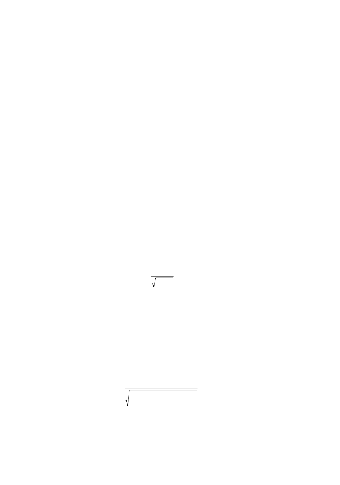
(1.23)

As we have seen in the Review, the sample mean is the most efficient unbiased estimator of the

population mean provided that the observations are independently drawn from the same distribution.

1.8 The Correlation Coefficient

In this chapter a lot of attention has been given to covariance. This is because it is very convenient

mathematically, not because it is a particularly good measure of association. We shall discuss its

deficiencies in this respect in Section 1.9. A much more satisfactory measure is its near-relative, the

correlation coefficient.

Like variance and covariance, the correlation coefficient comes in two forms, population and

sample. The population correlation coefficient is traditionally denoted

, the Greek letter that is the

equivalent of “r”, and pronounced “row”, as in row a boat. For variables

and

it is defined by

σσ

(1.24)

and

are independent,

will be equal to 0 because the population covariance will be 0. If

there is a positive association between them,

, and hence

, will be positive. If there is an exact

positive linear relationship,

will assume its maximum value of 1. Similarly, if there is a negative

relationship,

will be negative, with minimum value of –1.

The sample correlation coefficient,

, is defined by replacing the population covariance and

variances in (1.24) by their unbiased estimators. We have seen that these may be obtained by

multiplying the sample variances and covariances by

–1). Hence

)(Var

),(Cov

−−

−

(1.25)

The factors

–1) cancel, so we can conveniently define the sample correlation by

COVARIANCE, VARIANCE, AND CORRELATION

)(Var)(Var

),(Cov

(1.26)

, r has maximum value 1, which is attained when there is a perfect positive association

between the sample values of X and Y (when you plot the scatter diagram, the points lie exactly on an

upward-sloping straight line). Similarly, it has minimum value –1, attained when there is a perfect

negative association (the points lying exactly on a downward-sloping straight line). A value of 0

indicates that there is no association between the observations on X and Y in the sample. Of course the

fact that r = 0 does not necessarily imply that

= 0 or vice versa.

Illustration

We will use the education and earnings example in Section 1.1 to illustrate the calculation of the

sample correlation coefficient. The data are given in Table 1.1 and they are plotted in Figure 1.1. We

have already calculated Cov(S, Y) in Table 1.2, equal to 15.294, so we now need only Var(S) and

Var(Y), calculated in Table 1.3.

ABLE

1.3

Observation S Y

(S –

S )

(Y –

Y )

(S –

S )

(Y – Y )

(S – S )(Y –Y )

1 15 17.24 1.75 3.016 3.063 9.093 5.277

2 16 15.00 2.75 0.775 7.563 0.601 2.133

3 8 14.91 –5.25 0.685 27.563 0.470 –3.599

464.5–7.25 –9.725 52.563 94.566 70.503

5 15 18.00 1.75 3.776 3.063 14.254 6.607

6126.29–1.25 –7.935 1.563 62.956 9.918

7 12 19.23 –1.25 5.006 1.563 25.055 –6.257

8 18 18.69 4.75 4.466 22.563 19.941 21.211

9127.21–1.25 –7.015 1.563 49.203 8.768

10 20 42.06 6.75 27.836 45.563 774.815 187.890

11 17 15.38 3.75 1.156 14.063 1.335 4.333

12 12 12.70 –1.25 –1.525 1.563 2.324 1.906

13 12 26.00 –1.25 11.776 1.563 138.662 –14.719

14 9 7.50 –4.25 –6.725 18.063 45.219 28.579

15 15 5.00 1.75 –9.225 3.063 85.091 –16.143

16 12 21.63 –1.25 7.406 1.563 54.841 –9.257

17 16 12.10 2.75 –2.125 7.563 4.514 –5.842

18 12 5.55 –1.25 –8.675 1.563 75.247 10.843

19 12 7.50 –1.25 –6.725 1.563 45.219 8.406

20 14 8.00 0.75 –6.225 0.563 38.744 –4.668

Total 265 284.49 217.750 1,542.150 305.888

Average 13.250 14.225 10.888 77.108 15.294

COVARIANCE, VARIANCE, AND CORRELATION

From the last two columns of Table 1.3, you can see that Var(S) is 10.888 and Var(Y) is 77.108.

Hence

55.0

975.28

924.15

108.77888.10

924.15

r (1.27)

Exercises

1.5

In the years following the Second World War, the economic growth of those countries that had

suffered the greatest destruction, Germany and Japan, was more rapid than that of most other

industrialized countries. Various hypotheses were offered to explain this. Nicholas Kaldor, a

Hungarian economist, argued that the countries that had suffered the worst devastation had had to

invest comprehensively with new plant and equipment. Because they were using up-to-date

technology, their marginal costs were lower than those of their competitors in export markets, and

they gained market share. Because they gained market share, they needed to increase their

productive capacity and this meant additional investment, further lowering their marginal costs

and increasing their market share. Meanwhile those countries that had suffered least, such as the

U.S. and the U.K., had less need to re-invest. As a consequence the same process worked in the

opposite direction. Their marginal costs were relatively high, so they lost market share and had

less need to increase capacity. As evidence for this hypothesis, Kaldor showed that there was a

high correlation between the output growth rate, x, and the productivity growth rate, p, in the

manufacturing sectors in the 12 countries listed in the table.

When a critic pointed out that it was inevitable that x and p would be highly correlated,

irrespective of the validity of this hypothesis, Kaldor proposed a variation on his hypothesis.

Economic growth was initially high in all countries for a few years after the war, but in some,

particularly the U.S. and the U.K., it was soon checked by a shortage of labor, and a negative

cycle took hold. In others, like Germany and Japan, where agriculture still accounted for a large

share of employment, the manufacturing sector could continue to grow by attracting workers

from the agricultural sector, and they would then have an advantage. A positive correlation

between the growth rate of employment, e, and that of productivity would be evidence in favor of

his hypothesis.

Annual Growth Rates (%)

Employment Productivity

Austria 2.0 4.2

Belgium 1.5 3.9

Canada 2.3 1.3

Denmark 2.5 3.2

France 1.9 3.8

Italy 4.4 4.2

Japan 5.8 7.8

Netherlands 1.9 4.1

Norway 0.5 4.4

West Germany 2.7 4.5

U.K. 0.6 2.8

U.S. 0.8 2.6

COVARIANCE, VARIANCE, AND CORRELATION

The table reproduces his data set, which relates to the period 1953/1954 to 1963/1964

(annual exponential growth rates). Plot a scatter diagram and calculate the sample correlation

coefficient for e and p. [If you are not able to use a spreadsheet application for this purpose, you

are strongly advised to use equations (1.9) and (1.17) for the sample covariance and variance and

to keep a copy of your calculation, as this will save you time with another exercise in Chapter 2.].

Comment on your findings.

1.6

Suppose that the observations on two variables X and Y lie on a straight line

Y = b

+ b

Demonstrate that Cov(X, Y) = b

Var(X) and that Var(Y) =

b Var(X) , and hence that the sample

correlation coefficient is equal to 1 if the slope of the line is positive, –1 if it is negative.

1.7*

Suppose that a variable Y is defined by the exact linear relationship

Y = b

+ b

and suppose that a sample of observations has been obtained for X, Y, and a third variable, Z.

Show that the sample correlation coefficient for Y and Z must be the same as that for X and Z, if

is positive.

1.9 Why Covariance is Not a Good Measure of Association

The correlation coefficient is a much better measure of association than the covariance, the main

reason being that the covariance depends on the units in which the variables X and Y happen to be

measured, whereas the correlation coefficient does not. This will be demonstrated for the sample

concepts; the proof for the population concepts will be left as an exercise.

Returning to the schooling and earnings example, we will investigate what happens when hourly

earnings are measured in cents rather than dollars. The covariance will be affected, but the correlation

coefficient will not.

We will denote the revised earnings data by Y'. The data for S and Y' are shown in Table 1.4. Of

course the data for Y' are just the data for Y in Table 1.2, multiplied by 100. As a consequence, the

average value of Y' in the sample is 100 times as large as the average value of Y. When we come to

calculate the earnings deviations (Y' –

), these are 100 times those in Table 1.2 because (Y' –

) =

(100Y’ – 100

) = 100(Y –

). Hence the products (S – S ) (Y' –

) are 100 times those in Table

1.2 and the sample covariance, 1529.4, is 100 times that obtained when hourly earnings were

measured in dollars. However, the correlation coefficient is unaffected. The correlation coefficient

for S and Y' is

55.0

771080888.10

4.1529

)'(Var)(Var

)',(Cov

. (1.28)

COVARIANCE, VARIANCE, AND CORRELATION

ABLE

1.4

Observation S Y'

(S –

S )

(Y' –

'Y )

(S –

S )

(Y' – 'Y )

(S – S )(Y' – 'Y )

1 15 1724 1.75 301.6 3.063 90930 527.7

2 16 1500 2.75 77.5

7.563 6010

213.3

3 8 1491 –5.25 68.5

27.563 4700

–359.9

4 6 450 –7.25 –972.5

52.563 945660

7050.3

5 15 1800 1.75 377.6

3.063 142540

660.7

6 12 629 –1.25 –793.5

1.563 629560

991.8

7 12 1923 –1.25 500.6

1.563 250550

–625.7

8 18 1869 4.75 446.6

22.563 199410

2121.1

9 12 721 –1.25 –701.5

1.563 492030

876.8

10 20 4206 6.75 2783.6

45.563 7748150

18789.0

11 17 1538 3.75 115.6

14.063 13350

433.3

12 12 1270 –1.25 –152.5

1.563 23240

190.6

13 12 2600 –1.25 1177.6

1.563 1386620

–1471.9

14 9 750 –4.25 –672.5

18.063 452190

2857.9

15 15 500 1.75 –922.5

3.063 850910

–1614.3

16 12 2163 –1.25 740.6

1.563 548410

–925.7

17 16 1210 2.75 –212.5

7.563 45140

–584.2

18 12 555 –1.25 –867.5

1.563 752470

1084.3

19 12 750 –1.25 –672.5

1.563 452190

840.6

20 14 800 0.75 –622.5

0.563 387440

–466.8

Total 265 28449 217.750 15421500 30588.8

Average 13.25

14225 10.888 771080 1529.4

The numerator (the top half of the fraction) has been multiplied by 100, but so has the denominator

(the bottom half), since Var(Y') is 100

Var(Y). (Remember that, when you multiply a variable by a

constant, you multiply its variance by the constant squared.) The denominator is multiplied by 100,

rather than 100

, because Var(Y') is under a square root.

Exercise

1.8

Demonstrate that, in general, the sample correlation coefficient is not affected by a change in

the unit of measurement of one of the variables.



SIMPLE REGRESSION

ANALYSIS

This chapter shows how a hypothetical linear relationship between two variables can be quantified

using appropriate data. The principle of least squares regression analysis is explained, and expressions

for the coefficients are derived.

Most students taking an introductory econometrics course will already have taken a basic calculus

course and should have no trouble following the derivations of the regression coefficients. Those who

have not should skip Section 2.3 and the proof in Section 2.5. They will then have to take the

expressions on trust, but they should still be able to understand in general terms how the expressions

have been derived.

2.1 The Simple Linear Model

The correlation coefficient may indicate that two variables are associated with one another, but it does

not give any idea of the kind of relationship involved. We will now take the investigation a step

further in those cases for which we are willing to hypothesize than one variable depends on another.

It must be stated immediately that one would not expect to find an exact relationship between any

two economic variables, unless it is true as a matter of definition. In textbook expositions of economic

theory, the usual way of dealing with this awkward fact is to write down the relationship as if it were

exact and to warn the reader that it is really only an approximation. In statistical analysis, however,

one generally acknowledges the fact that the relationship is not exact by explicitly including in it a

random factor known as the disturbance term.

We shall start with the simplest possible model:

. (2.1)

, the value of the dependent variable in observation

, has two components: (1) the nonrandom

component

being described as the explanatory (or independent) variable, and the fixed

quantities

and

as the parameters of the equation, and (2) the disturbance term,

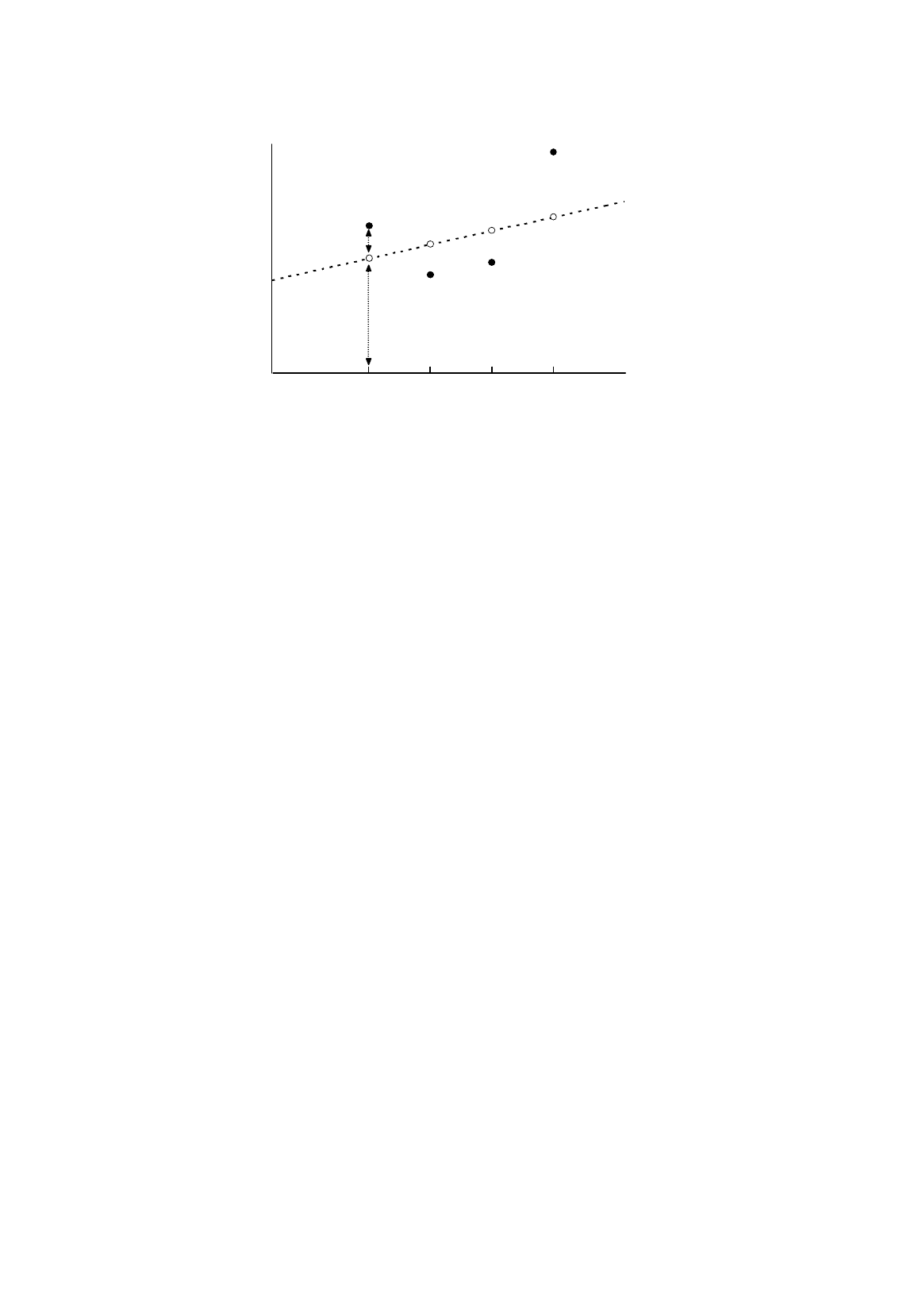
Figure 2.1 illustrates how these two components combine to determine

, and

are

four hypothetical values of the explanatory variable. If the relationship between

and

were exact,

the corresponding values of

would be represented by the points

–

on the line. The disturbance

term causes the actual values of

to be different. In the diagram, the disturbance term has been

assumed to be positive in the first and fourth observations and negative in the other two, with the

result that, if one plots the actual values of

against the values of

, one obtains the points

–

SIMPLE REGRESSION ANALYSIS

Figure 2.1.

True relationship between

and

It must be emphasized that in practice the P points are all one can see of Figure 2.1. The actual

values of

and

, and hence the location of the Q points, are unknown, as are the values of the

disturbance term in the observations. The task of regression analysis is to obtain estimates of

and

, and hence an estimate of the location of the line, given the P points.

Why does the disturbance term exist? There are several reasons.

1. Omission of explanatory variables: The relationship between Y and X is almost certain to be a

simplification. In reality there will be other factors affecting Y that have been left out of (2.1),

and their influence will cause the points to lie off the line. It often happens that there are

variables that you would like to include in the regression equation but cannot because you are

unable to measure them. For example, later on in this chapter we will fit an earnings function

relating hourly earnings to years of schooling. We know very well that schooling is not the

only determinant of earnings and eventually we will improve the model by including other

variables, such as years of work experience. However, even the best-specified earnings

function accounts for at most half of the variation in earnings. Many other factors affect the

chances of obtaining a good job, like the unmeasurable attributes of an individual, and even

pure luck in the sense of the individual finding a job which is a good match for his or her

attributes. All of these other factors contribute to the disturbance term.

2. Aggregation of variables: In many cases the relationship is an attempt to summarize in

aggregate a number of microeconomic relationships. For example, the aggregate consumption

function is an attempt to summarize a set of individual expenditure decisions. Since the

individual relationships are likely to have different parameters, any attempt to relate aggregate

expenditure to aggregate income can only be an approximation. The discrepancy is attributed

to the disturbance term.

3. Model misspecification: The model may be misspecified in terms of its structure. Just to give

one of the many possible examples, if the relationship refers to time series data, the value of Y

may depend not on the actual value of X but on the value that had been anticipated in the

previous period. If the anticipated and actual values are closely related, there will appear to be

SIMPLE REGRESSION ANALYSIS

a relationship between Y and X, but it will only be an approximation, and again the disturbance

term will pick up the discrepancy.

4. Functional misspecification: The functional relationship between Y and X may be misspecified

mathematically. For example, the true relationship may be nonlinear instead of linear. We will

consider the fitting of nonlinear relationships in Chapter 5. Obviously, one should try to avoid

this problem by using an appropriate mathematical specification, but even the most

sophisticated specification is likely to be only an approximation, and the discrepancy

contributes to the disturbance term.

5. Measurement error: If the measurement of one or more of the variables in the relationship is

subject to error, the observed values will not appear to conform to an exact relationship, and

the discrepancy contributes to the disturbance term.

The disturbance term is the collective outcome of all these factors. Obviously, if you were

concerned only with measuring the effect of X on Y, it would be much more convenient if the

disturbance term did not exist. Were it not for its presence, the P points in Figure 2.1 would coincide

with the Q points, you would know that every change in Y from observation to observation was due to

a change in X, and you would be able to calculate

and

exactly. However, in fact, part of each

change in Y is due to a change in u, and this makes life more difficult. For this reason, u is sometimes

described as noise.

2.2 Least Squares Regression

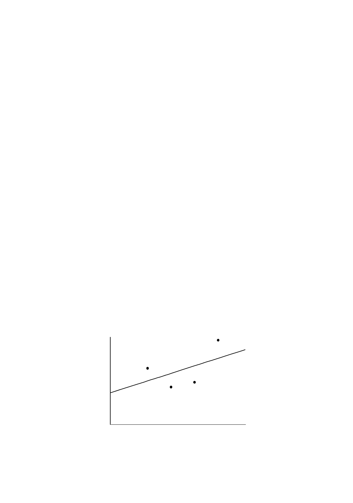
Suppose that you are given the four observations on X and Y represented in Figure 2.1 and you are

asked to obtain estimates of the values of

and

in equation (2.1). As a rough approximation, you

could do this by plotting the four P points and drawing a line to fit them as best you can. This has been

done in Figure 2.2. The intersection of the line with the Y-axis provides an estimate of the intercept

which will be denoted b

, and the slope provides an estimate of the slope coefficient

, which will be

denoted b

. The fitted line will be written

Figure 2.2.

Fitted line

SIMPLE REGRESSION ANALYSIS

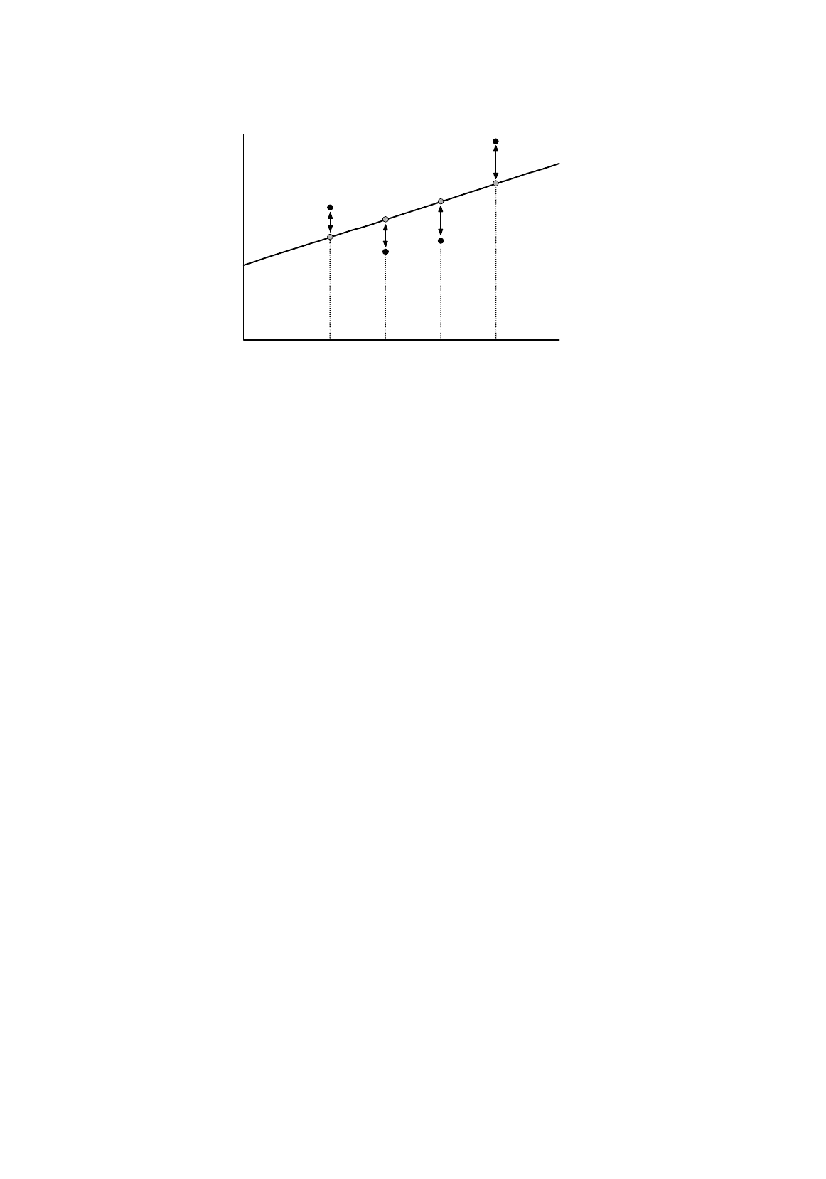
Figure 2.3.

Fitted regression line showing residuals

XbbY

(2.2)

the caret mark over

indicating that it is the fitted value of

corresponding to

, not the actual value.

In Figure 2.3, the fitted points are represented by the points

–

One thing that should be accepted from the beginning is that you can never discover the true

values of

and

, however much care you take in drawing the line.

and

are only estimates, and

they may be good or bad. Once in a while your estimates may be absolutely accurate, but this can only

be by coincidence, and even then you will have no way of knowing that you have hit the target

exactly.

This remains the case even when you use more sophisticated techniques. Drawing a regression

line by eye is all very well, but it leaves a lot to subjective judgment. Furthermore, as will become

obvious, it is not even possible when you have a variable

depending on two or more explanatory

variables instead of only one. The question arises, is there a way of calculating good estimates of

and

algebraically?

The first step is to define what is known as a residual for each observation. This is the difference

between the actual value of

in any observation and the fitted value given by the regression line, that

is, the vertical distance between

and

in observation

. It will be denoted

iii

YYe

−=

(2.3)

The residuals for the four observations are shown in Figure 2.3. Substituting (2.2) into (2.3), we

obtain

–

(2.4)

and hence the residual in each observation depends on our choice of

and

. Obviously, we wish to

fit the regression line, that is, choose

and

, in such a way as to make the residuals as small as

SIMPLE REGRESSION ANALYSIS

possible. Equally obviously, a line that fits some observations well will fit others badly and vice versa.

We need to devise a criterion of fit that takes account of the size of all the residuals simultaneously.

There are a number of possible criteria, some of which work better than others. It is useless

minimizing the sum of the residuals, for example. The sum will automatically be equal to 0 if you

make b

equal to

and b

equal to 0, obtaining the horizontal line Y =

. The positive residuals will

then exactly balance the negative ones but, other than this, the line will not fit the observations.

One way of overcoming the problem is to minimize RSS, the sum of the squares of the residuals.

For Figure 2.3,

eeeeRSS

+++=

(2.5)

The smaller one can make RSS, the better is the fit, according to this criterion. If one could reduce

RSS to 0, one would have a perfect fit, for this would imply that all the residuals are equal to 0. The

line would go through all the points, but of course in general the disturbance term makes this

impossible.

There are other quite reasonable solutions, but the least squares criterion yields estimates of b

and b

that are unbiased and the most efficient of their type, provided that certain conditions are

satisfied. For this reason, the least squares technique is far and away the most popular in

uncomplicated applications of regression analysis. The form used here is usually referred to as

ordinary least squares and abbreviated OLS. Variants designed to cope with particular problems will

be discussed later in the text.

2.3 Least Squares Regression: Two Examples

Example 1

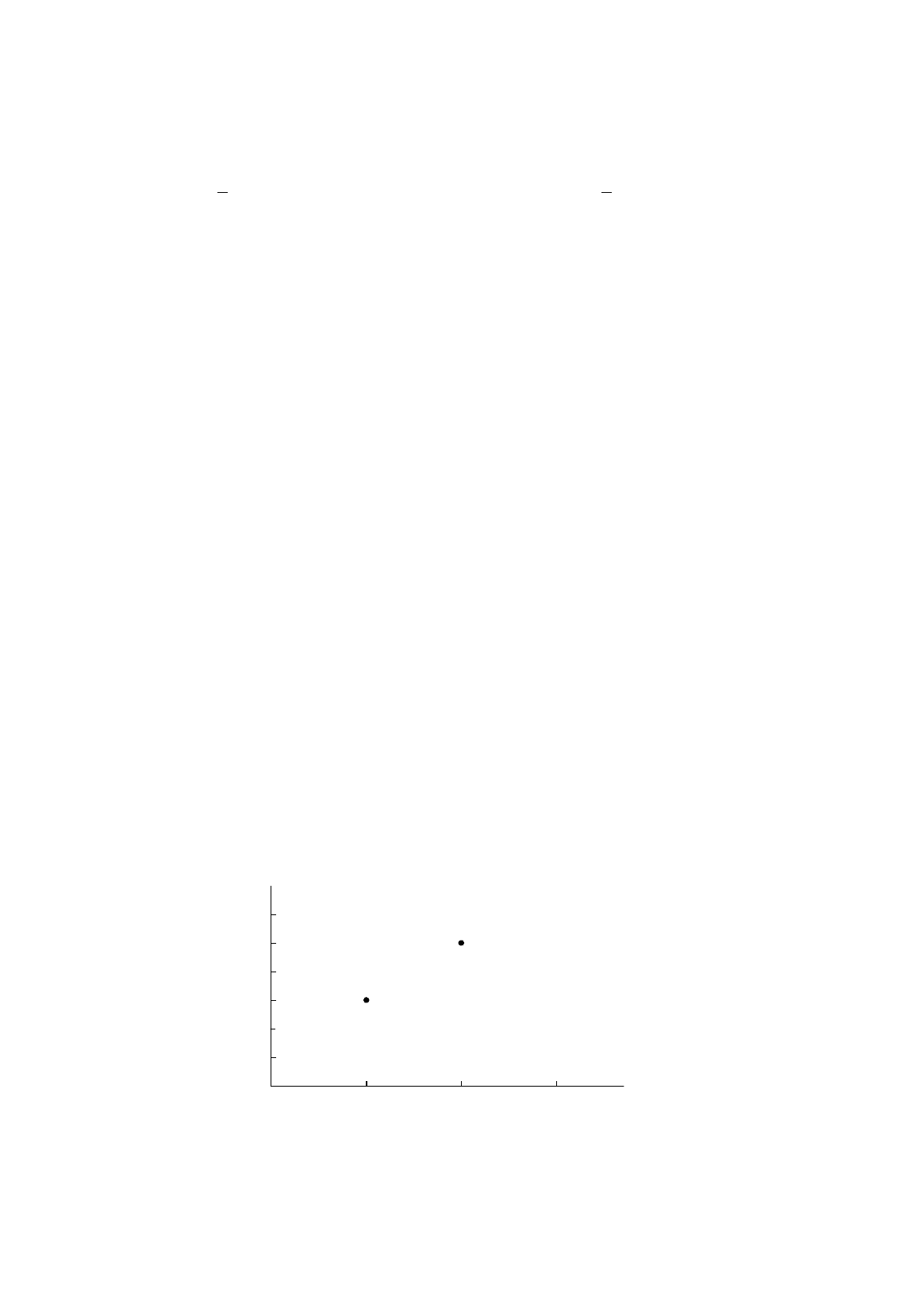
First, a very simple example indeed, with only two observations, just to show the mechanics working.

Y is observed to be equal to 3 when X is equal to 1; Y is equal to 5 when X is equal to 2, as shown in

Figure 2.4.

Two-observation example

123