Dougherty С. Introduction to Econometrics, 3Ed
Подождите немного. Документ загружается.


BINARY CHOICE MODELS AND MAXIMUM LIKELIHOOD ESTIMATION
23
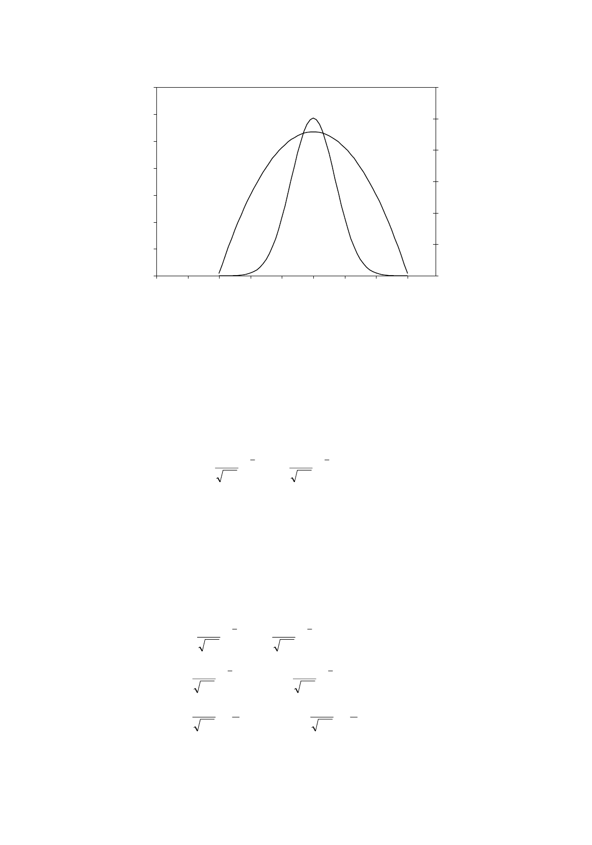
Figure 11.13.
Probability densities at
X
1
= 4 and
X
2
= 6 conditional on
µ
= 4.0.
Table 11.3 computes the probabilities of X = 4 and X = 6 for values of
µ
from 3.5 to 6.5. The
fourth column gives the joint probability density, which is known as the likelihood function. The
likelihood function is plotted in Figure 11.14. You can see that it reaches a maximum for
µ
= 5, the
average value of the two observations. We will now demonstrate mathematically that this must be the
case.
T
ABLE
11.3
µ
p(4 |
µ
) p(6 |
µ
)
L log L
3.5 0.3521 0.0175 0.0062 –5.0879
4.0 0.3989 0.0540 0.0215 –3.8379
4.5 0.3521 0.1295 0.0456 –3.0879
4.6 0.3332 0.1497 0.0499 –2.9979
4.7 0.3123 0.1714 0.0535 –2.9279
4.8 0.2897 0.1942 0.0563 –2.8779
4.9 0.2661 0.2179 0.0580 –2.8479
5.0 0.2420 0.2420 0.0585 –2.8379
5.1 0.2179 0.2661 0.0580 –2.8479
5.2 0.1942 0.2897 0.0563 –2.8779
5.3 0.1714 0.3123 0.0535 –2.9279
5.4 0.1497 0.3332 0.0499 –2.9979
5.5 0.1295 0.3521 0.0456 –3.0879
6.0 0.0540 0.3989 0.0215 –3.8379
6.5 0.0175 0.3521 0.0062 –5.0879
0.0
0.1
0.2
0.3
0.4
012345678
µ
p
0.3989
0.0540
BINARY CHOICE MODELS AND MAXIMUM LIKELIHOOD ESTIMATION
24
Figure 11.14.
Likelihood and log-likelihood functions for
µ
.
First, a little terminology. The likelihood function, written L(
µ
| X
1
= 4, X
2
= 6) gives the joint
probability density as a function of
µ
, given the sample observations. We will choose
µ
so as to
maximize this function.
In this case, given the two observations and the assumption
σ
= 1, the likelihood function is given
by
() ()
=
−−−−
22
6
2
1
4
2
1
2
1
2
1
)(
µµ
ππ
µ
eeL
(11.26)
We will now differentiate this with respect to
µ
and set the result equal to 0 to obtain the first-
order condition for a maximum. We will then differentiate a second time to check the second-order
condition. Well, actually we won’t. Even with only two observations in the sample, this would be
laborious, and when we generalize to n observations it would be very messy. We will use a trick to
simplify the proceedings. log L is a monotonically increasing function of L. So the value of
µ
that
maximizes L also maximizes log L, and vice versa. log L is much easier to work with, since
22
)6(
2
1
)4(
2
1
)6(
2
1
)4(
2
1
)6(
2
1
2
1
log)4(
2
1
2
1
log
2
1
log
2
1
log
2
1
2
1
loglog
22
22
µ
π
µ
π
ππ
ππ
µµ
µµ
−−
+−−
=
+
=
=
−−−−
−−−−
ee
eeL
(11.27)
µ
0.00
0.01
0.02
0.03
0.04
0.05
0.06
0.07
012345678
Likelihood
-12
-10
-8
-6
-4
-2
0
Log-likelihood
Log-likelihood
function
Likelihood function

BINARY CHOICE MODELS AND MAXIMUM LIKELIHOOD ESTIMATION
25
The maximum likelihood estimator, which we will denote
µ
ˆ
, is the value of
µ
that maximizes
this function, given the data for X. It is given by the first-order condition
0)
ˆ
6()
ˆ
4(
log
=−+−=
µ
µ
µ
d
Ld
(11.28)
Thus
µ
ˆ
= 5. The second derivative is –2, so this gives a maximum value for log L, and hence L.
[Note that
222
2
1
2
1
)(
2
1
µ
µ
µ
−+−=−−
aaa
. Hence the differential with respect to
µ
is (a –
µ
).]
Generalization to a Sample of n Observations
Consider a sample that consists of n observations X
1
, …, X
n
. The likelihood function L(
µ
| X
1
, …, X
n
)
is now the product of n terms:
() ()
××
=
−−−−
22
1
2
1
2
1
2
1
...
2
1
)(
µµ
ππ
µ
n
XX
eeL (11.29)
The log-likelihood function is now the sum of n terms:
22
1
)(
2
1
)(
2
1
)(
2
1
2
1
log...)(
2
1
2
1
log
2
1
log...
2
1
loglog
22
1
µ
π
µ
π
ππ
µµ
−−
++−−
=
++
=
−−−−
n
XX
XX
eeL
n
(11.30)
Hence the maximum likelihood estimator of
µ
is given by
0)
ˆ
(...)
ˆ
(
log
1
=−++−=
µ
µ
µ
n
XX
d
Ld
(11.31)
Thus
∑
=
n
i
i
X
1
– n
µ
= 0 (11.32)
and the maximum likelihood estimator of
µ
is the sample mean. Note that the second derivative is –n,
confirming that the log-likelihood has been maximized.
BINARY CHOICE MODELS AND MAXIMUM LIKELIHOOD ESTIMATION
26
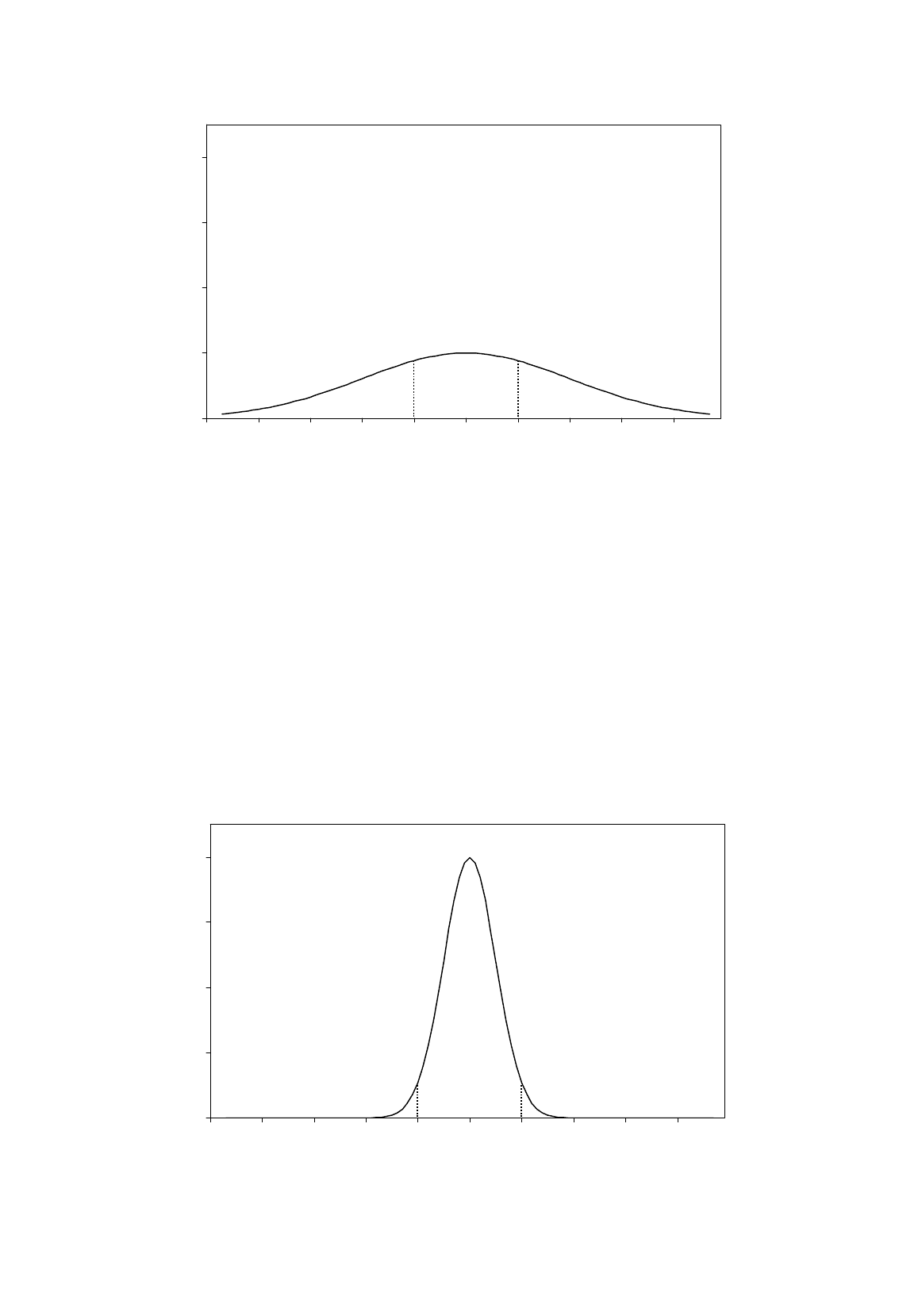
Figure 11.15.
Probability densities at
X
1
= 4 and
X
2
= 6 conditional on
σ
= 2.
Generalization to the Case Where
σ
is Unknown.
We will now relax the assumption that
σ
is equal to 1 and accept that in practice it would be unknown,
like
µ
. We will investigate the determination of its maximum likelihood graphically using the two-
observation example and then generalize to a sample of n observations.
Figure 11.15 shows the probability distribution for X conditional on
µ
being equal to 5 and
σ
being equal to 2. The probability density at X
1
= 4 and X
2
= 6 is 0.1760 and the joint density 0.0310.
Clearly we would obtain higher densities, and higher joint density, if the distribution had smaller
variance. If we try
σ
equal to 0.5, we obtain the distribution shown in Figure 11.16. Here the
Figure11.16.
Probability densities at
X
1
= 4 and
X
2
= 6 conditional on
σ
= 0.5.
0.0
0.2
0.4
0.6
0.8
0123456789
p
µ
0.1760 0.1760
0.0
0.2
0.4
0.6
0.8
0123456789
0.1080 0.1080
µ
p
BINARY CHOICE MODELS AND MAXIMUM LIKELIHOOD ESTIMATION
27
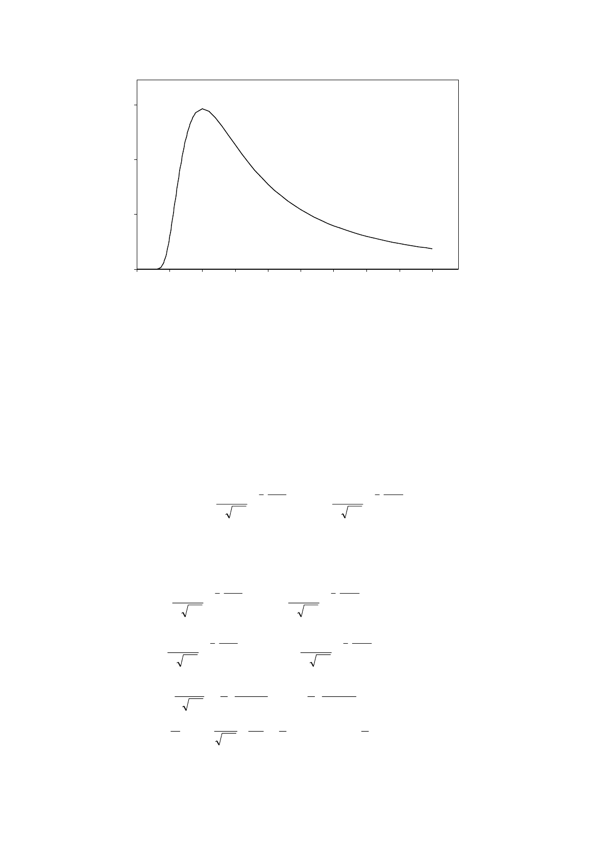
Figure 11.17.
Likelihood function for
σ
.
individual densities are 0.1080 and the joint density 0.0117. Clearly we have made the distribution too
narrow, for X
1
and X
2
are now in its tails with even lower density than before.
Figure 11.17 plots the joint density as a function of
σ
. We can see that it is maximized when
σ
is
equal to 1, and this is therefore the maximum likelihood estimate, provided that we have been correct
in assuming that the maximum likelihood estimate of
µ
is 5.
We will now derive the maximum likelihood estimators of both
µ
and
σ
simultaneously, for the
general case of a sample of n observations. The likelihood function is
L(
µ
,
σ
|
××
=
−
−
−
−
2
2
1
2
1
2
1
1
2
1
...
2
1
),...,
σ
µ
σ
µ
πσπσ
n
X
X
n
eeXX (11.33)
and so the log-likelihood function is
−−−−−++=
−
−−
−
−
=
++
=
××
=
−
−
−
−
−
−
−
−
22
1
2
2
2
1
2
1
2
1
2
1
2
1
)(
2
1
...)(
2
11
2
1
log
1
log
2
1
...
2
1
2
1
log
2
1
log...
2
1
log
2
1
...
2
1
loglog
2
2
1
2
2
1
µ
µ
σ
π
σ
σ
µ
σ
µ
πο
πσπσ
πσπσ
σ
µ
σ
µ
σ
µ
σ
µ
n
n
X
X
X
X
XXnn
X
X
n
ee
eeL
n
n
(11.34)
0
0.02
0.04
0.06
0 0.5 1 1.5 2 2.5 3 3.5 4 4.5
σ
L

BINARY CHOICE MODELS AND MAXIMUM LIKELIHOOD ESTIMATION
28
The partial derivative of this with respect to
µ
is
[]
)(...)(
1log
1
2
µ
µ
σ
µ
−++−=
∂
∂
n
XX
L
(11.35)
Setting this equal to 0, one finds that the maximum likelihood estimator of
µ
is the sample mean,
as before. The partial derivative with respect to
σ
is
∑
=
−+−
n
i
i
X
n
1
2
3
)(
1
µ
σ
σ
(11.36)
Substituting its maximum likelihood estimator for
µ
, and putting the expression equal to 0, we
obtain
∑
=
−=
n
i
i
XX
n
1
22
)(
1
ˆ
σ
(11.37)
Note that this is actually biased downwards in finite samples, the unbiased estimator being given
by the same expression with
n
replaced by (
n
– 1). However it is asymptotically more efficient using
the mean square error criterion, its smaller variance more than compensating for the bias. The bias in
any case attenuates as the sample size becomes large.
Application to the Simple Regression Model
Suppose that
Y
i
depends on
X
i
according to the simple relationship
Y
i
=
β
1
+
β
2
X
i
+
u
i
(11.38)
Potentially, before the observations are generated,
Y
i
has a distribution around (
β
1
+
β
2
X
i
),
according to the value of the disturbance term. We will assume that the disturbance term is normally
distributed with mean 0 and standard deviation
σ
, so
2
2
1
2
1
)(
−
=
σ
πσ
u
euf
(11.39)
The probability that
Y
will take a specific value
Y
i
in observation
i
is determined by the
probability that
u
i
is equal to (
Y
i
–
β
1
–
β
2
X
i
). Given the expression above, the corresponding
probability density is
2
21
2
1
2
1
−−
−
σ
ββ
πσ
ii
XY
e
(11.40)

BINARY CHOICE MODELS AND MAXIMUM LIKELIHOOD ESTIMATION
29
The joint probability density function for the observations in the sample is the product of the
terms for each observation. Taking the observations as given, and treating the unknown parameters as
variables, we say that the likelihood function for
β
1
,
β
2
and
σ
is given by
××
=
−−
−
−−
−
2
21
2
1211
2
1
2
1
121
2
1
...
2
1
),...,|,,(
σ
ββ
σ
ββ
πσπσ
σ
β
β
nn
XY
XY
n
eeYYL
(11.41)
The log-likelihood function is thus given by
()( )
[]
2
21
2
1211
...
2
1
2
1
loglog
nn
XYXYnL
β
β
β
β
σ
πσ
−−++−−−
=
(11.42)
The values of
β
1
and
β
2
that maximize this function are exactly the same as those obtained using the
least squares principle. However, the estimate of
σ
is slightly different.
Goodness of Fit and Statistical Tests
As noted in the discussion of logit analysis, there is no measure of goodness of fit equivalent to
R
2
in
maximum likelihood estimation. The pseudo-
R
2
seen in some regression output, including that of
Stata, compares its log-likelihood, log
L
, with the log-likelihood that would have been obtained with
only the intercept in the regression, log
L
0
. A likelihood, being a joint probability, must lie between 0
and 1, and as a consequence a log-likelihood must be negative. The pseudo-
R
2
is the proportion by
which log
L
is smaller, in absolute size, than log
L
0
:
pseudo-
R
2
= 1 –
0
log
log
L
L
(11.43)
While it has a minimum value of 0, its maximum value must be less than 1 and unlike
R
2
it does not
have a natural interpretation. However variations in the likelihood, like variations in the residual sum
of squares in a standard regression, can be used as a basis for tests. In particular the explanatory
power of the model can be tested via the likelihood ratio statistic
2 log
0
L
L
= 2(log
L
– log
L
0
) (11.44)
is distributed as a chi-squared statistic with
k
- 1 degrees of freedom, where
k
- 1 is the number of
explanatory variables, under the null hypothesis that the coefficients of the variables are all jointly
equal to 0. Further, the validity of a restriction can be tested by comparing the constrained and
unconstrained likelihoods, in the same way that it can be tested by comparing the constrained and
unconstrained residual sum of squares in a least squares regression model. For example, the null
hypothesis
H
0
:
ρ
= 0 in the selection bias model can be tested by comparing the unconstrained
likelihood
L
U
with the likelihood
L
R
when the model is fitted assuming that
u
and
ε
are distributed

BINARY CHOICE MODELS AND MAXIMUM LIKELIHOOD ESTIMATION
30
independently. Under the null hypothesis H
0
:
ρ
= 0, the test statistic 2 log
R
U
L
L
is distributed as a chi-
squared statistic with one degree of freedom. In the example in Section 11.4, the test statistic, 32.90,
appears in the last line of the output and the null hypothesis is rejected, the critical value of
χ
2
(1) being
10.83 at the 0.1 percent level.
As was noted in Section 11.2, the significance of an individual coefficient can be evaluated via its
asymptotic t statistic, so-called because the standard error is valid only in large samples. Since the t
distribution converges on the normal distribution in large samples, the critical values of the latter
should be used.
Exercises
11.8*
An event is hypothesized to occur with probability p. In a sample of n observations, it
occurred m times. Demonstrate that the maximum likelihood estimator of p is m/n.
11.9* In Exercise 11.4, log L
0
is the log-likelihood reported on iteration 0. Compute the pseudo-R
2
and confirm that it is equal to that reported in the output.
11.10* In Exercise 11.4, compute the likelihood ratio statistic 2(log L – log L
0
), confirm that it is
equal to that reported in the output, and perform the likelihood ratio test.
C. Dougherty 2001. All rights reserved. Copies may be made for personal use. Version of 16.05.01.
12
MODELS USING
TIME SERIES DATA
Hitherto the analysis has been confined to cross-section data. With samples being taken from fixed
populations, it has been reasonable to assume that the classical linear regression model is the
appropriate framework. Now we switch to time series data and data generation processes. In this
chapter and the next we will suppose that the classical linear regression model remains a suitable
vehicle. However in the final chapter we shall see that analysis using times series data involves new
problems and requires a different approach.
12.1 Static Models
Much of the analysis will be illustrated with a core data set for fitting demand functions. It is drawn
from national accounts data published by the U.S. Bureau of the Census and consists of annual
aggregate data on 24 different categories of consumer expenditure for the period 1959–1994, along
with data on disposable personal income,
DPI
, and price index numbers for the 24 categories. The
Demand Functions data set, together with a manual giving more detailed information about it, can be
downloaded from the website. It will be updated periodically, so the time period covered will be
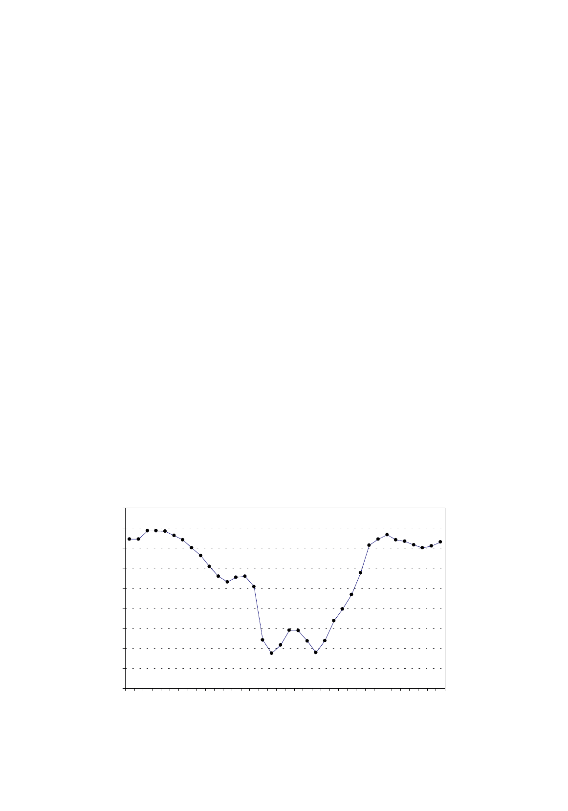
Figure 12.1.
Relative price series for housing services, 1959–1994 (1992=100)
86
88
90
92
94
96
98
100
102
104
1959 1963 1967 1971 1975 1979 1983 1987 1991

MODELS USING TIME SERIES DATA
2
extended and possibly there may be changes to the categories of consumer expenditure. Two of the
categories, FOOD and HOUS (consumer expenditure on food and housing services, respectively) are
used as examples in the text and exercises. The other categories are intended for practical work by a
small group of students, each student working with a different category, starting with a simple
regression specification and gradually developing a more sophisticated one. We will start with a very
simple specification for the demand equation for housing services, regressing consumer expenditure
on this category, HOUS, on DPI and a price index for housing, PRELHOUS:
HOUS
t
=
β
1
+
β
2
DPI
t
+
β
3
PRELHOUS
t
+
u
t
(12.1)
HOUS
and
DPI
are measured in $ billion at 1992 constant prices.
PRELHOUS
is an index
constructed by dividing the nominal price deflator for housing,
PHOUS
, by the price deflator for total
personal expenditure,
PTPE
, and multiplying by 100.
PRELHOUS
thus is a real or relative price
index that keeps track of whether housing is becoming more or less expensive relative to other types
of expenditure. It is plotted in Figure 12.1, which shows that the relative price declined by about 10
percent from the early 1960s to the late 1970s and then rose again by about the same amount.
A straightforward linear regression using EViews gives the following output (standard errors in
parentheses):
=============================================================
Dependent Variable: HOUS
Method: Least Squares
Sample: 1959 1994
Included observations: 36
=============================================================
Variable Coefficient Std. Error t-Statistic Prob.
=============================================================
C 2.654701 28.91571 0.091808 0.9274
DPI 0.151521 0.001243 121.9343 0.0000
PRELHOUS -0.556949 0.290640 -1.916285 0.0640
=============================================================
R-squared 0.997811 Mean dependent var 429.3306
Adjusted R-squared 0.997679 S.D. dependent var 149.1037
S.E. of regression 7.183749 Akaike info criter 4.023298
Sum squared resid 1703.006 Schwarz criterion 4.155258
Log likelihood -120.5012 F-statistic 7522.482
Durbin-Watson stat 0.809993 Prob(F-statistic) 0.000000
=============================================================
The equation implies that an increase of $1 billion in disposable personal income leads to an
increase of $0.15 billion in expenditure on housing. In other words, out of the marginal dollar, 15
cents is spent on housing. Is this a plausible figure? It is a bit difficult to tell, but certainly housing is
the largest category of consumer expenditure and one would expect a substantial coefficient. Note that
we are talking about housing services, and not investment in housing. Housing services is the value of
the services provided by the existing housing stock. In the case of rented housing, rents are taken as a
measure of the value of the services. In the case of owner-occupied housing and housing rented at a
subsidized rate, imputed rents, that is, the market rents the housing could command, are used instead.
The coefficient of
PRELHOUS
implies that a one-point increase in the price index leads to a reduction
of $0.56 billion in expenditure on housing. The constant term literally indicates the amount that would
be spent on housing if
DPI
and
PRELHOUS
were both 0, but obviously any such interpretation is
nonsense. If the observations referred to households, there might be some that had no income and yet
purchased housing services and other essentials with transfer payments, but here we are talking about
