Dorst L., Fontijne D., Mann S. Geometric Algebra for Computer Science. An Object Oriented Approach to Geometry

Подождите немного. Документ загружается.

SECTION 3.11 PROGRAMMING EXAMPLES AND EXERCISES 97

// get ’white’ vector:

e3ga::vector white = _vector(unit_e(e1 + e2 + e3));

// Get two vectors, orthogonal to white:

// factorizeBlade() find two vectors such that

// dual(white) == O[1] ^ O[2]

e3ga::vector O[2];

factorizeBlade(dual(white), O);

/**

Converts colors in ’source’ images to ’dest’ image, according

to the input color frame ’IFcolors’. Reciprocal vectors are returned

in ’RFcolors’.

void colorSpaceConvert(

const unsigned char *source,

unsigned char *dest,

unsigned int width, unsigned int height,

const e3ga::vector *IFcolors,

e3ga::vector *RFcolors) {

// compute reciprocal frame

reciprocalFrame(IFcolors, RFcolors, 3);

for (unsigned int i = 0; i < (width * height) * 3; i += 3) {

// convert RGB pixel to vector:

e3ga::vector c(vector_e1_e2_e3, (float)source[i + 0], (float)source[i + 1],

(float)source[i + 2]);

// compute colors in in destination image:

float red = _Float(c << g_RFcolors[0]);

float green = _Float(c << g_RFcolors[1]);

float blue = _Float(c << g_RFcolors[2]);

// clip colors:

if (red < 0.0f) red = 0.0f;

else if (red > 255.0f) red = 255.0f;

if (green < 0.0f) green = 0.0f;

else if (green > 255.0f) green = 255.0f;

if (blue < 0.0f) blue = 0.0f;

else if (blue > 255.0f) blue = 255.0f;

// set colors in destination image

dest[i + 0] = (unsigned char)(red + 0.5f); // +0.5f for correct rounding

dest[i + 1] = (unsigned char)(green + 0.5f);

dest[i + 2] = (unsigned char)(blue + 0.5f);

}

Figure 3.12: Color space conversion code (Example 4).

98 METRIC PRODUCTS OF SUBSPACES CHAPTER 3

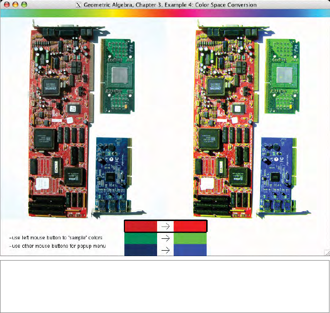
Figure 3.13: Color space conversion screenshot (Example 4). On the left is the original

image: a photo of some computer parts that contains red, green, and blue patches. On the right

is an example of a converted image: the colors of the parts have been converted to “pure”

red, green, and blue.

We now have a frame which spans the RGB color space. We can generate all fully saturated

colors by performing a rotation in the

O[0] ∧ O[1]-plane:

// alpha runs from 0 to 2 PI

for (float angle = 0.0f; angle < PI2; angle += STEP) {

// generate all fully saturated colors:

e3ga::vector C = _vector(white + cos(angle) * O[0] +

sin(angle) * O[1]);

// set current color:

glColor3fv(C.getC(vector_e1_e2_e3));

// draw small patch in the current color:

// ...

}

LINEAR TRANSFORMATIONS

OF SUBSPACES

Linear transformations of a vector space R

change its vectors. When this happens,

the blades spanned by those vectors change quite naturally to become the spans of the

transformed vectors. That deﬁnes the extension of a linear transformation to the full sub-

space algebra. This embedding gives us more powerful tools to apply linear transforma-

tions immediately to subspaces, without needing to ﬁrst decompose those subspaces into

vectors.

We study the resulting structure in this chapter. The algebra dictates how we should do

the outer products and contractions of transformed blades, and in that way gives us the

transformation formulas for the products themselves. Transforming contractions is a lot

more involved than transforming outer products (since it involves the metric of the space),

but the effort pays off by providing a compact coordinate-free formula for the inverse of

a linear transformation.

In this book we will mostly be interested in orthogonal transformations. We can

easily derive some of their properties in this chapter and see why they are special (they

are the only transformations that are structure-preserving for the contraction). Their real

importance and ease of representation will be revealed only in Chapter 7.

At ﬁrst reading, you can skim through this chapter, taking in only the principle of the

outermorphism, which takes the structure preservation of the outer product as its tenet

and the transformation formulas for the other products. The main facts are summarized

in Section 4.6.

100 LINEAR TRANSFORMATIONS OF SUBSPACES CHAPTER 4

f[αx]

f[x]

αx

x + y

x ∧ y

f[x ∧ y]

f[x]

f[y]

f[x + y]

(a) (b)

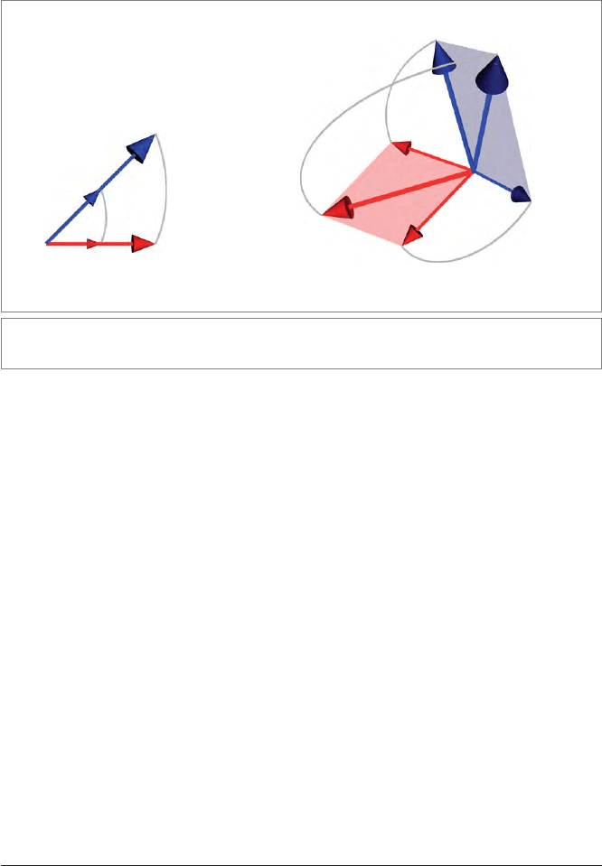
Figure 4.1: The deﬁning properties of a linear transformation.

4.1 LINEAR TRANSFORMATIONS OF VECTORS

We are interested in linear transformations, mapping a vector space R

onto itself.

Such

a linear transformation f :

→ R

has the deﬁning properties

f[α x + β y] = αf[x] + βf[y],

(4.1)

where α,β ∈

R are scalars and x, y ∈ R

are vectors. It is convenient to see this as two

conditions:



f[α x] = αf[x]

f[x + y] = f[x] + f[y]

(4.2)

The ﬁrst condition means that a line through the origin remains a straight line through the

origin, with a preservation of ratios of vectors along the lines (Figure 4.1(a)). The second

condition means that the parallelogram-based addition is preserved (see Figure 4.1(b)).

Examples of such linear transformations on subspaces include scaling, rotation (but only

around an axis through origin), and reﬂection (but only relative to subspace containing

the origin), but not translation, which tends to produce nonhomogeneous, offset spaces.

1 In this chapter, we perform linear transformations within the same space R

, not from one space to another.

Though the same principles apply to both, the additional notation involved in such space-to-space transformations

would hide the basic structural simplicity we need to expose here.

SECTION 4.2 OUTERMORPHISMS: LINEAR TRANSFORMATIONS OF BLADES 101

Linear transformations therefore do not include certain important transformations that

we deﬁnitely want to include in our treatment of geometry. Yet linear transformations are

important, because we will see in Part II how we can construct those desirables using linear

transformations in higher-dimensional operational models of afﬁne or Euclidean space.

Also, linear mappings provide a local description of a wide class of arbitrary mappings,

which is a successful way to study those in differential geometry.

4.2 OUTERMORPHISMS: LINEAR

TRANSFORMATIONS OF BLADES

We start with a speciﬁc linear transformationfin the vector space R

, which maps vectors

to vectors. We will use sans serif type to denote these linear transformations to distinguish

them from the blades (and other elements we introduce later), and denote their action

by square brackets to avoid confusion with the grouping brackets of the products, and

remind ourselves of their linearity. Sof[x] denotes the action of the linear transformation

f on the vector x.

We would like to ﬁnd a natural extension that makes f act on arbitrary blades, or even

arbitrary multivectors. We will argue that this natural extension should be done according

to the following simple rules:

f[α] = α for scalar α

f[A ∧ B] = f[A] ∧f[B]

f[A + B] = f[A] + f[B]

(4.3)

where A and B are blades of arbitrary grade (even grade 0), although the results imme-

diately generalize to general multivectors by the imposed linearity. (The third rule is a

consequence of the second and (4.2), at least for same-grade blades, but we prefer to have

it explicit so that linearity can be easily extended to multivectors.)

An extension of a map of vectors to vectors in this manner to the whole of the Grass-

mann algebra is called extension as a (linear) outermorphism, since the second property

shows that we obtain a morphism (i.e., a mapping) that commutes with the outer prod-

uct. The properties in (4.3) fully deﬁne the outermorphism corresponding to the linear

transformation f.

Outermorphisms have nice algebraic properties that are essential to their geometrical

usage:

•

Blades Remain Blades. Geometrically, oriented subspaces are transformed to

oriented subspaces.

•

Grades Are Preserved. The linear transformation f turnsvectorsintovectors.Then

it follows immediately from the second rule that grade(f[A]) = grade(A) for blades.

102 LINEAR TRANSFORMATIONS OF SUBSPACES CHAPTER 4

Geometrically, this means that the dimensionality of subspaces does not change

under a linear transformation.

•

Preservation of Factorization.IfA and B have a blade C in common (so that they

may be written as A = A



∧ C and B = C ∧ B



, for appropriately chosen A



and B



then f[A] and f[B] have f[C] in common. Geometrically, this means that the

meet

(intersection) of subspaces is preserved.

If you are happy with (4.3) as a deﬁnition, you can move on to Section 4.2.2. If you need

some motivation to convince yourself of its consistency with the algebra of subspaces as

we developed it thus far, read the next section.

4.2.1 MOTIVATION OF THE OUTERMORPHISM

Let us take a step back from the algebraic generalization of a linear transformation in (4.3)

and show its geometric plausibility.

In the beginning, we have nothing more than the linear transformation f from vectors

to vectors f :

→ R

. It obviously satisﬁes the linearity axioms of (4.2), graphically

depicted in Figure 4.1.

We want linear transformations on all k-blades. Starting with 2-blades, we introduce a

linear transformation f

mapping 2-blades to 2-blades (i.e., f



→



Linearity of f

now means linearity for 2-blades, so satisfying f

[αA] = αf

[A] and

[A + B] = f

[A] + f

[B] —whereA and B are 2-blades. But this mapping f

cannot be

totally arbitrary. One way to construct the 2-blades is by using two vectors. If A = x ∧ y,

how should we relate f (acting on vectors in

)tof

(acting on 2-blades in



), so

that we get a consistent structure to our subspace algebra? Figure 4.1 provides the clue:

the parallelogram construction is preserved under f by the linearity axioms—and such

a construction occurs not only in deﬁning the sum of vectors, but also in deﬁning the 2-

blade through the outer product (compare Figure 2.2 to Figure 2.3(a)). So we must connect

the two linear transformations f and f

in a structurally consistent manner by setting

[x ∧ y] = f[x] ∧f[y].

This 2-blade is linear in x and y, and so are both sides of this equation, guaranteeing that

the construction is internally consistent. For instance: f

[α(x ∧ y)] = f

[(α x) ∧ y] =

f[α x] ∧f[y] = αf[x] ∧f[y] = αf

[x ∧ y], which is a proof that f

thus deﬁned indeed

has one of the linearity properties. Since it is so consistent, we can consider f and f

the same linear transformation, just overloaded to apply to arguments of different grade,

so we denote them both by f.

The story for 3-blades is similar—the parallelepiped construction can be interpreted as

a span (outer product) or as an addition diagram (linearity). Equating the two suggests

deﬁning

SECTION 4.2 OUTERMORPHISMS: LINEAR TRANSFORMATIONS OF BLADES 103

f[x ∧ y ∧ z] = f[x] ∧f[y] ∧f[z].

Associativity of the outer product gives us associativity for the outermorphismf, and then

f naturally extends to all grades.

There is also a strong suggestion of how we should relate a linear transformation among

scalars (i.e., 0-blades) to the linear transformation f of vectors in a consistent manner.

Remember that by (2.5), the standard product of a vector with a scalar is just the outer

product in disguise. As a consequence, the ﬁrst linearity condition of (4.2) can be read

in our exterior algebra as f[α ∧ x] = α ∧f[x]. To keep the outermorphism property, it is

therefore natural to deﬁne

f[α] = α

as the extension of f to scalars. The geometric semantics of this is that the point at the

origin remains ﬁxed under a linear transformation, in all its qualities, including weight

and sign.

This is how the whole ladder of subspaces is affected naturally by the linear transformation

of the underlying vector space, preserving the structure of the spanning product that went

into its construction: the span of the transforms is the transform of the span.

4.2.2 EXAMPLES OF OUTERMORPHISMS

Let us look at some simple examples of such extensions of linear transformations.

1. Uniform Scaling. This is the linear transformation S[x] = αx.Onann-blade A =

∧ a

∧···∧a

, this gives

S[A] = S[a

] ∧ S[a

] ∧···∧S[a

] = α

(4.4)

For 2-blades represented as parallelograms, this contains the well-known result that

as each of the sides is multiplied by α, the area is multiplied by α

; but it is more, since

it also contains the statement that the attitude of the 2-blade remains the same, and

so does its orientation, even when α is negative. And since 2-blades have no ﬁxed

shape, the same applies to any area in the plane: as the linear measure gets scaled by

α, the area measure scales by α

For a 3-blade I

= a

∧ a

in 3-D space, we obtain S[I

] = α

,asexpected.

When α is negative, there is thus an orientation change of the volume. Again, noth-

ing shatteringly new in its geometric interpretation, but note how in the formulation

of such statements, their computation and their proof are all an intrinsic part of the

algebra at a very elementary level. That is how we would want it.

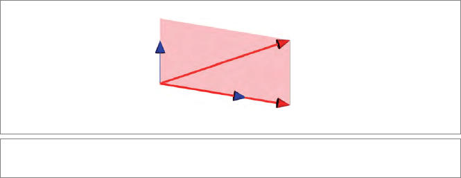
2. Parallel Projection onto a Line. In the plane with 2-blade a ∧b, let the linear trans-

formation P be such that P[a] = a, while P[b] = 0. This is a projection in the

b-direction onto the a-line (see Figure 4.2). Since any vector x in this plane can be

written as an a-component plus a b-component, this determines the transformation

104 LINEAR TRANSFORMATIONS OF SUBSPACES CHAPTER 4

P[x]

Figure 4.2: Projection onto a line a in the b-direction.

P[x] = P[α a + β b] = α a (4.5)

(where α can be computed as (x∧b)/(a∧b) using the reciprocal frame of Section 3.8

or the techniques of Section 2.7.1). Extending this P as an outermorphism, we ﬁnd

that P[a ∧ b] = P[a] ∧ P[b] = a ∧ 0 = 0. Any 2-blade in the plane a ∧ b becomes 0:

this transformation makes areas disappear.

You may have expected the answer to be P[a ∧ b] = P[a], because intuitively the

plane a∧b becomes the line a. But this is not what an outermorphism does (it always

preserves grade), so we must be careful with such na

ıve geometrical motivations for

the results of algebraic computations. The image of the plane of vectors is indeed

the line of vectors, but the plane of vectors is not equivalent to the 2-blade of the

plane!

3. Planar Rotation. Consider two independent unit vectors u and v that span a 2-blade

u ∧v. This 2-blade determines a plane through the origin in a Euclidean space

n,0

Let R be a rotation around the origin in this plane, a linear transformation. Let the

rotation be such that it turns u to v,soR[u] = v. Since the whole plane rotates,

the vector originally at v also rotates to a unit vector w ≡ R[v]. Since the rotation

around the origin is linear, the parallelogram spanned by u and v transforms to

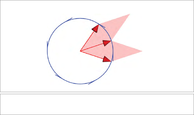
another parallelogram spanned by v = R[u] and w = R[v] (see Figure 4.3). The

sketch shows that u ∧ v and v ∧ w are identical 2-blades, so u ∧ v = v ∧ w. This

permits us to compute the effect of the rotation on a 2-blade:

R[u ∧ v] = R[u] ∧ R[v] = v ∧ w = u ∧ v.

(4.6)

It follows that the 2-blade u ∧ v is preserved under the rotation. This corresponds

well to our insight that a rotation plane is an invariant of a rotation. But note

how speciﬁc (4.6) is: it states that all properties of the plane—attitude, area mea-

sure, and orientation—are preserved. It is remarkable that although the vectors

SECTION 4.2 OUTERMORPHISMS: LINEAR TRANSFORMATIONS OF BLADES 105

v ∧ w

u ∧ v

Figure 4.3: A rotation around the origin of unit vectors in the plane of the page, described

by 2-blades.

u and v themselves are not preserved (they rotate), their 2-blade is. We might

express this as a rotation has no real eigenvectors in its plane, but it has a real

eigenblade of grade 2: the plane itself.

Note that we have not speciﬁed any space in which we perform the rotation,

assuming only that it has as least 2 dimensions for the 2-blade to be nonzero. So

our picture and reasoning apply to any space of more than 1 dimension.

4. Point Reﬂections. In a point reﬂection through the origin, all vectors change sign.

So this is a uniform scaling by −1. Then (4.4) shows that an n-blade changes by

(−1)

: blades of even grades are unchanged, and blades of odd grades obtain the

opposite orientation. Note that this does not depend on the dimensionality of the

space in which they are embedded. As an example, point reﬂection in 3-D space

changes the orientation of 3-blades, that is, the handedness of objects: a right-hand

glove becomes a left-hand glove (see also structural exercise 1). We will see soon that

this cannot be undone by a rotation, using an argument that only involves the outer

product.

5. Orthogonal Projection. In (3.25) we met the orthogonal projection of a vector x

onto a blade B as P

[x] =



(xB)B

−1



. Since the mapping is linear, we can extend

it as an outermorphism to construct the projection of a higher-order subspace X

onto B. Let us ﬁrst extend this orthogonal projection from the vector x to the bivec-

tor x∧y. By outermorphism, the projection of (x∧y) onto B should be P

[x]∧P

[y].

Now we have a straightforward derivation in which we challenge you to identify the

rewriting rules.

106 LINEAR TRANSFORMATIONS OF SUBSPACES CHAPTER 4

[x] ∧ P

[y] =



(xB)B

−1



∧



(yB)B

−1





(xB)B

−1



(yB)



B

−1



(xB)B

−1



∧ y



B



B

−1

= −



y ∧



(xB)B

−1



B



B

−1

= −



y



(xB)B

−1



B



B

−1

= −



y



(xB) ∧ (B

−1

B)



B

−1

= −



y(xB)



B

−1

= −



(y ∧ x)B



B

−1



(x ∧ y)B



B

−1

= P

[x ∧ y].

The ﬁnal result is, therefore, that we can just apply the projection formula directly

to the blade x∧y to get the outermorphism. Similar steps can be used to provide an

inductive proof of the general result for blades of (3.26).

Geometrically, the outermorphism property implies that the projection formula

generalizes to higher-order blades in a pleasant way. Our algebra permits the direct

projection of subspaces without the necessity of breaking them up into vectors, pro-

jecting those, and recomposing the result.

These examples show how merely having the outer product already reﬁnes and extends

our analysis and application of linear transformations.

4.2.3 THE DETERMINANT OF A LINEAR TRANSFORMATION

We have seen in Chapter 2 how in an n-dimensional space, the blade of highest grade

that can be constructed without being identical to 0 is an n-blade, which is a pseudoscalar

for the space. The grade-preservation property of a linear transformation f implies that a

linear transformation on a pseudoscalar I

produces another pseudoscalar. Moreover, all

pseudoscalars are scalar multiples of each other, since the space of n-blades



is a 1-D

linear space. Therefore we ﬁnd f[I

] = δ I

, with δ a scalar. This deﬁnes δ as the change

in pseudoscalar magnitude and orientation, as a ratio of the transformed n-dimensional

hypervolume (for that is what a pseudoscalar is) to the original hypervolume. It is called

the determinant of f, denoted det(f). So we have the important implicit deﬁnition

determinant : f[I

] ≡ det (f) I

(4.7)

This scalar number det(f) is indeed equivalent in value to that concept in linear algebra, so

we are not abusing the name. There, too, the determinant is a ratio of signed hypervolume

measures.

The usual way of teaching linear algebra in the applied sciences relies heavily on matrix

representations. You might be excused for believing that linear algebra is about matrices