Daniels M.J., Hogan J.W. Missing Data in Longitudinal Studies: Strategies for Bayesian Modeling and Sensitivity Analysis

Подождите немного. Документ загружается.

160 CASE STUDIES: IGNORABLE MISSINGNESS

Table 7.12 CTQ II: posterior means of diﬀerence in quit rates with 95% credible

intervals at week 8 for each ofthethreemodelsconsidered. Observed-data sample

means included for comparison.

Model Posterior Mean 95% C.I.

A-MAR .08 (.00, .16)

MAR .08 (.00, .16)

Independence .03 (–.06, .10)

Observed .04

population-level variation in CD4 before and after initiation of HAART. Here

we present a comparative analysis based on p-splines.

7.6.1 Models

Deﬁne Y

to be the J

-dimensional vector of CD4 counts measured at times

,...,t

i,J

). We model the CD4 trajectories using p-splines (see Examples

2.7 and 3.10) with linear (q =1)andquadratic(q =2)basesusing a multi-

variate normal model with an exponential covariance function

| X

∼ N (X

β, Σ

where the elements σ

ikl

(φ)ofΣ

take the form

ikl

= σ

exp(−φ

−t

). (7.3)

The matrices x

are speciﬁed using a truncated power basis with 18 equally

spaced knots placed at the sample quantiles of the observation times. So, the

jth row is given by

= {1,t

,...,t

, (t

− s

)

, (t

− s

)

,...,(t

− s

)

}

where {s

,...,s

} are the knots and β is partitioned as

β =(α

,α

,...,α

,...,a

)

=(α

, a

)

In this study, not all the data were observed and the observed data were

irregularly spaced. The analysis here implicitly assumes that the unobserved

data are MAR.

HERS CD4 DATA 161

7.6.2 Priors

Bounded uniform priors are speciﬁed for the residual standard deviation σ

and the correlation parameter φ for the exponential covariance function in

(7.3), with lower bounds of 0 and upper bounds of 100 and 10, respectively.

The components of the (q +1)-dimensional vector of coeﬃcients α are given

‘just proper’ independent normal priors with mean 0 and variance 10

;the

coeﬃcients corresponding to the knots a are given normal priors with mean

zero and variance τ

.Thestandard deviation τ is then given a Unif(0, 10)

prior.

7.6.3 MCMC details

Three chains wereruneachfor15, 000 iterations with a burn-in of 5000. The

autocorrelation in the chains was minimal.

7.6.4 Model selection

In addition to the model with an exponential covariance function for the

residuals, we also ﬁt a model that assumes independent residuals (φ =0)for

comparison. To assess ﬁt among the models, we computed the DIC with θ =

(β,φ,1/σ

, 1/τ

); see Table 7.13. The best-ﬁtting model was the quadratic

p-spline with the exponential covariance function. The greatly improved ﬁt

of both the linear and quadratic p-splines with residual autocorrelation over

independence of the residuals is clear from the large diﬀerences in the DIC.

Table 7.13 HERS CD4 data: DIC under q =1, q =2(linear and quadratic spline

bases), under independence and exponential covariance functions.

Model DIC Dev(θ) p

Independence, q =1 19417 19400 8

Independence, q =2 19417 19402 7

Exponential, q =1 18008 17985 11

Exponential, q =2 17999 17980 9

7.6.5 Results

Posterior means and 95% credible intervals for the covariance parameters

in the best-ﬁtting model (as measured by the DIC) with q =2appear in

162 CASE STUDIES: IGNORABLE MISSINGNESS

Table 7.14. The correlation parameter φ was signiﬁcantly diﬀerent from zero,

with the posterior mean corresponding to a lag 1 (week) correlation of .52.

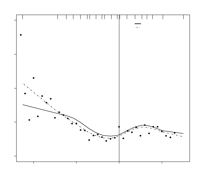
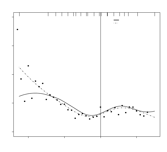
Posterior means of the curves for q =1andq =2appear in Figures 7.2 and

7.3, respectively.

The posterior mean of the spline curves were relatively similar for q =1and

q =2andcaptured more local variation thantheindependence models; time

zero on the plot represents self-reported initiation of HAART. An increase

can be seen near self-reported initiation (the eﬀect of HAART), followed by a

decrease later on, possibly attributable to noncompliance and development of

resistantviral strains. The results also suggest that the self-reports of HAART

initiation are subject to a delay relative to the actual initiation of HAART

because the decrease in CD4 levels occurs prior to self-reported initiation time

(t =0).

Table 7.14 Posterior means and 95% credible intervals for exponential covariance

function parameters and smoothing standard deviation under q =2for the HERS

CD4 data.

Parameter Posterior Mean 95% C.I.

φ .65 (.60, .70)

σ 3.9 (3.8, 4.0)

τ 1.9 (.81, 3.6)

7.7 Summary

The ﬁve examples in this chapter have demonstrated a variety of fundamental

concepts for properly modeling incomplete data under an assumption of ignor-

ability. The importance of correctly specifying the dependence structure was

emphasized in all the examples and approaches for choosing the best-ﬁtting

model and assessing the ﬁt of such models under ignorability using DIC

and

posterior predictive checks were demonstrated.

In addition, we illustrated the use of joint modeling to properly address

auxiliary stochastic time-varying covariates when an assumption of auxiliary

variable MAR (A-MAR) is thought plausible.

Under ignorability, model speciﬁcation only involved the full data response

model. In the next three chapters we discuss model-based approaches for

nonignorable missing data that require speciﬁcation of the full-data model,

i.e., the full-data response model and the missing data mechanism (explicitly).

In Chapter 10 we present threedetailed case studies.

SUMMARY 163

−2000 −1000 0 1000

200 400 600 800 1000

Time since HAART initiation

CD4 count

exponential covariance

naive independence

Figure 7.2 HERS CD4 data: plot of observed data with ﬁtted p-spline curve with

q =1under independence and exponential covariance function. The observed data

(dots) are averages over 100 day windows. The tick marks on the top of the plot

denote percentiles.

164 CASE STUDIES: IGNORABLE MISSINGNESS

−2000 −1000 0 1000

200 400 600 800 1000

Time since HAART initiation

CD4 count

exponential covariance

naive independence

Figure 7.3 HERS CD4 data: plot of observed data with ﬁtted p-spline curve with

q =2under independence and exponential covariance function. The observed data

(dots) are averages over 100 day windows. The tick marks on the top of the plot

denote percentiles.

CHAPTER 8

Models for Handling Nonignorable

Missingness

8.1 Overview

This chapter covers many of the central concepts and modeling approaches

for dealing with nonignorable missingness and dropout. A prevailing theme

is the factorization of the full-data model into the observed data distribution

and the extrapolation distribution, wherethelatter characterizes assumptions

about the conditional distribution of missing data given observed information

(observed responses, missing data indicators, and covariates). The extrapo-

lation factorization (as we refer to it) factors the full-data distribution into

its identiﬁed and nonidentiﬁed components. We argue that models for non-

ignorable dropout should be parameterized in such a way that one or more

parameters for the extrapolation distribution is completely nonidentiﬁed by

data. These also should have transparent interpretation so as to facilitate sen-

sitivity analysis or incorporation of prior information about the missing data

distribution or missing data mechanism.

In Section 8.2, we describe the extrapolation distribution and state con-

ditions for parameters to be sensitivity parameters.Section 8.3 reviews se-

lection models, with particular emphasis on how the models are identiﬁed.

We show that parametric selection models cannot be factored into identi-

ﬁed and nonidentiﬁed parts, resulting in an absence of sensitivity parameters.

Semiparametric selection models are introduced as a potentially useful alter-

native. Section 8.4 covers mixture models for both discrete and continuous

responses, and for discrete and continuous dropout times. We show that in

many cases, mixture models are easily factored using the extrapolation factor-

ization, enabling interpretable sensitivity analyses and formulation of missing

data assumptions. Computation of covariate eﬀects for mixture models also is

discussed. Section 8.5 provides an overview of shared parameters models. In

Section 8.6, we provide a detailed discussion of possible approaches to model

selection and model ﬁt. This is still an open area of research, and our coverage

highlights several of the key conceptual and technical issues. Model ﬁt and

model selection under nonignorable missingness diﬀer from the ignorable case

because with nonignorability, the full-data distribution includes a speciﬁca-

tion for f (r | y)thatmustbechecked against observed r. Suggestions for

further reading are given in Section 8.7.

165

166 NONIGNORABLE MISSINGNESS

8.2 Extrapolation factorization and sensitivity parameters

In Chapter 5, we introduced a classiﬁcation of dropout mechanisms that, with

respect to posterior inference, can be classiﬁed as ignorable or nonignorable.

In Chapter 6, we reviewed and discussed concepts and models for ignorable

dropout, and illustrated using case studies in Chapter 7. In this chapter, we

describe several diﬀerent models for nonignorable dropout that are character-

ized via speciﬁcation of the full data distribution f(y, r | ω).

Recall that the full data distribution can be factored into an extrapolation

model and an observed data model,

p(y, r | ω)=p(y

mis

| y

obs

, r, ω

) p(y

obs

, r | ω

Here, ω

and ω

denote parameters indexing the extrapolation and observed

data models, respectively. They are potentially, but not necessarily, overlap-

ping functions of ω.Theobserved data distribution p(y

obs

,r | ω

), is identi-

ﬁed and can (in principle) be estimated nonparametrically. The extrapolation

distribution p(y

mis

| y

obs

, r, ω

)cannotbeidentiﬁedwithoutmodelingas-

sumptions or constraints on the parameter space.

In general we advocate using parameterizations in which one or more pa-

rameters indexing the extrapolation cannot be identiﬁed by observed data.

To formalize this notion, we deﬁne a class of parameters for full-data models

that can be used for sensitivity analysisorincorporation of informative prior

information. Generally they are not identiﬁable from observed data, but when

their values are ﬁxed, the remainder of the full-data model is identiﬁed. For-

mally we call them sensitivity parameters and in general, we use the term to

mean parameters that satisfy this deﬁnition.

Deﬁnition 8.1. Sensitivity parameter.

Let p(y, r | ω)denoteafull-data model. Its extrapolation factorization is

given by

p(y, r | ω)=p(y

mis

| y

obs

, r, ω

) p(y

obs

, r | ω

If there exists a reparameterization ξ(ω)=(ξ

, ξ

)suchthat:

1. ξ

is a nonconstant function of ω

2. the observed-data likelihood

L(ξ

, ξ

| y

obs

, r)

is constant as afunction of ξ

,and

3. at a ﬁxed value of ξ

,theobserved data likelihood is a nonconstant

function of ξ

then ξ

is a sensitivity parameter. 2

The ﬁrst condition requires that ξ

be a nonconstant function of the param-

eters of the extrapolation distribution. The second condition implies that the

SELECTION MODELS 167

ﬁt of the model to the observed data is not aﬀected by the sensitivity parame-

ters. In any particular full-data model, there may be several sets of parameters

that satisfy the ﬁrst two conditions. However, there will often be only one set

that satisﬁes the third condition as well, which states when the sensitivity

parameters are ﬁxed, the full data model is identiﬁed. These conditions will

be helpful in determining sensitivity parameters for semiparametric selection

models in Section 8.3.7. For mixture models, ﬁnding sensitivity parameters is

usually very easy (see Section 8.4.3).

The framework we use is very similar to the one based on nonparametric

identiﬁed (NPI) full-data models proposed by Robins (1997) and discussed in

some detail by Vansteelandt et al. (2006). A class M (γ)offull-data models is

nonparametric identiﬁed if, for an observed data distribution p(y

obs

, r), there

exists a unique full-data model p(y

obs

, y

mis

, r | γ) ∈ M (γ)thatmarginalizes

to p(y

obs

, r); i.e.



p(y

obs

, y

mis

, r | γ) dy

mis

= p(y

obs

, r).

The observed data donotcontain information about γ, but knowing γ points

toaspeciﬁcp(y

obs

, y

mis

, r | γ)intheclassM (γ)thatcoincideswithp(y

obs

, r).

Vansteelandt et al. (2006) call γ asensitivityparameter if it indexes a NPI

class of full-data models M (γ).

Deﬁnition 8.1 is designed for the likelihood framework, but essentially pos-

sesses the same attributes. In short, sensitivity parameters index the missing

data extrapolation and cannot be identiﬁed by observed data. They provide

the framework for assessing sensitivity of model-based inferences to assump-

tions about the missing data mechanism, or incorporating those assumptions

formally in terms of informative prior distributions.

As it turns out, not all models are amenable to this type of parametriza-

tion. Parametric selectionmodelsinparticularcannot generally be factored

to permit sensitivity parameterizations. Mixture models tend to be easier to

work with. For models described below, we provide examples of parameteri-

zations that satisfy Deﬁnition 8.1, or indicate when they are diﬃcult or even

impossible to ﬁnd.

8.3 Selection models

In most of this section, we assume a common set, {t

,...,t

},ofobservation

times and without loss of generality t

= j.

8.3.1 Background and history

Recall from Chapter 5 that the selectionmodelfactors the full-data distribu-

tion as

p(y, r | ω)=p(r | y, ψ(ω)) p(y | θ(ω)); (8.1)

168 NONIGNORABLE MISSINGNESS

this factorization underlies the missing data taxonomy described in Section 5.4.

The typical strategy to model the two components is to specify a parametric

model for each and to assume that ψ and θ are distinct. In the following, we

will assume ψ and θ are distinct and aprioriindependent unless stated oth-

erwise. Note that this does not correspond to the (ω

, ω

)partition in (8.1).

An early example of selection modeling for multivariate data can be found

in Heckman(1979), where the joint distribution of a bivariate response Y

with missing Y

was speciﬁed using a multivariate normal distribution (im-

plicitly, a probit model for the binary indicators of missingness that is linear in

)

). Diggle and Kenward (1994) expanded the Heckman model to the

case of dropout in longitudinal studies using a logistic model for the hazard

of dropout. Many subsequent articles adapted and extended their approach

within a likelihood framework (see, e.g.,Fitzmaurice, Molenberghs, and Lip-

sitz, 1995; Baker, 1995; Molenberghs, Kenward, and Lesaﬀre, 1997; Liu, Wa-

ternaux, and Petkova, 1999; Albert, 2000; Heagerty and Kurland 2004). A

framework for semiparametric inference can be found in Robins et al. (1995)

and Scharfstein et al. (1999).

We begin our review of parametric selection models by demonstrating via

several examples the diﬃculty in ﬁnding sensitivity analysis parameteriza-

tions.

8.3.2 Absence of sensitivity parameters in the missing data mechanism

In many parametric selection models, all the parameters are identiﬁed. Iden-

tiﬁcation is drivenbyparametric assumptions on both the full-data response

model and the missing data mechanism (MDM).

To illustrate using a simple example, consider a cross-sectional setting

where Y may or may not be missing. Suppose the histogram of the observed

y’s looks like that given in Figure 8.1 and that we specify the following model

for the missing data mechanism:

logit{P (R =1| y)} = ψ

+ ψ

where R =1corresponds to observing Y .Withnofurtherassumptions about

the distribution of Y ,wecannot identify ψ

because when R =0,wedo

not observe Y .Itcan also be shown (Scharfstein et al., 2003) that ψ

is a

sensitivity parameter.

However, suppose we further assume that the full-data response model is

anormaldistribution, N(µ, σ

). By looking at the histogram of the observed

y’s in Figure 8.1, it is clear that for this histogram to be consistent with

normally distributed full-data y’s, we need to ﬁll in the right tail; this implies

< 0. On the other hand, if we assumed a parametric model for the full-data

response model that was consistent with the histogram for the observed y’s

(e.g., a skew-normal), it would suggest that ψ

=0.Thus,inference about

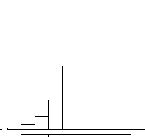
SELECTION MODELS 169

depends heavily on the distributional assumptions about p(y), and ψ

in fact identiﬁed by observed data. Hence it does not meet the criteria in

Deﬁnition 8.1, and therefore is not a sensitivity parameter.

Frequency

−3 −2 −1 0 1

050100 150

Figure 8.1 Histogram of observed responses.

This univariate example extends readily to the longitudinal setting. For

example, consider a bivariate normal full-data response having missingness in

,withmissing data mechanism

logit{P (R =1| y)} = ψ

+ ψ

, (8.2)

where R =1corresponds to observing Y

.Under a bivariate normal distribu-

tion for the full-data response model, the same argument used above would

be applicable in terms of the conditional distribution, p(y

| y

)andtheiden-

tiﬁcation of ψ

Sensitivity of MDM parameters to assumptions on the full-data response