Daniels M.J., Hogan J.W. Missing Data in Longitudinal Studies: Strategies for Bayesian Modeling and Sensitivity Analysis

Подождите немного. Документ загружается.

170 NONIGNORABLE MISSINGNESS

model was studied in a simple but very informative empirical example by Ken-

ward (1998). He considered a bivariate full-data response with Y

potentially

missing and missing data mechanism given in (8.2), and assessed the sensi-

tivity of inference about ψ to distributional assumptions about p(y

| y

). If

this distribution was assumed to be normal, the estimates and standard errors

of ψ implied MNAR. However, if this distribution was assumed to follow a

t-distribution with only a few degrees of freedom, the estimates and standard

errors of ψ implied MAR. So by just changing the tails of the distribution

of the full-data response, inference concerning the missing data mechanism

changedsigniﬁcantly. This and the previous hypothetical examples illustrate

the prominent role of modeling assumptions in parametric selection models:

widely diﬀering conclusions can be drawn based on unveriﬁable modeling as-

sumptions about the full-data response.

The preceding discussion has focused entirely on the full-data response

model in identifying potential sensitivity parameters in the missing data mech-

anism. However, we have focusedonthesimple(andcommon) situation where

the response y is entered into the MDM linearly. This is a strong assumption

and is not always appropriate. For example, in the schizophrenia clinical trial

(Section 1.2), it is conceivable that participants may be more likely to drop out

when they are doing much better or much worse, suggesting thatthemissing

data mechanism should be quadratic in y.Revisiting the previous example

with cross-sectional data, assume p(y

obs

)follows the histogram in Figure 8.1,

p(y)isanormaldistribution, and the MDM follows

logit{P (R =1| y)} = ψ

+ ψ

y + ψ

. (8.3)

This scenario is consistent with an MNAR mechanism having ψ

< 0and

=0,because the right tail needs to be ﬁlled in for the full-data responses

to be normally distributed (the left tail is already consistent with a normal

distribution). Alternatively, suppose that p(y

obs

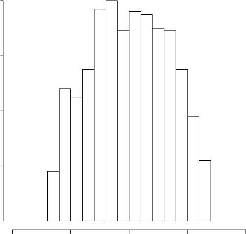
)resembled the histogram

in Figure 8.2. The quadratic MDM (8.3) is now consistent with ψ

> 0,

which is MNAR. On the other hand, with the same observed data response

distribution, an MDM that is linear in y (ψ

=0)isconsistent with ψ

=0,

which is MAR.

These simpleexamplesdemonstrate that for a fully speciﬁed parametric

selection model, all parameters are identiﬁed. Asaconsequence, there are no

obvious sensitivity parameters. By contrast, in an ideal sensitivity analysis, the

distribution of Y

mis

given Y

obs

and R is governed by parameters that aﬀect

the full-data distribution but not the observed-data distribution, so that per-

turbations of these parameter values do not aﬀect ﬁt of the full-data model

to observables. By this criterion, parametric selection models are not well-

suited to sensitivity analysis or to incorporation of prior information about

p(y

mis

| y

obs

, r). A detailed discussion of this point follows in Sections 8.3.3

through 8.3.6; in Section 8.3.7 we introduce semiparametric selection mod-

SELECTION MODELS 171

Frequency

−2 −1 0 1 2

020406080

Figure 8.2 Histogram of observed responses.

els, which oﬀer a more viable selection-model-based framework for sensitivity

analysis.

8.3.3 Heckman selection model for a bivariate response

We start out our review of parametric selection models by providing details

on the Heckman model (Heckman, 1979). Let Y =(Y

)

denote a bivari-

ate outcome,andletR be an indicator of whether Y

is observed (R =1

corresponds to Y

being observed). Heckman proposed to jointly model the

172 NONIGNORABLE MISSINGNESS

outcome and missingness using a trivariate normal distribution as follows:













∼ N





































. (8.4)

In this setup, Z is a continuous latent variable underlying the missingness

indicator, where R = I{Z>0}.Thismodelimplies Y ∼ N (µ

, Σ

), where

is the upper left 2 × 2submatrix of the covariance matrix in (8.4). The

Heckman model requires some restrictions on the the σ

,whichwedetail

below.

Let Γ = Σ

−1

,anddenote the unique elements of Γ by {γ

,γ

The selection model above implies that the missing data mechanism follows

aprobitregression that is linear in Y

and Y

P (R =1| y)=P (Z>0 | y)=Φ(ψ

+ ψ

). (8.5)

Referring to (8.4),

= µ

− ψ

= σ

+ σ

= σ

+ σ

Note that the regression parameters in the missing data mechanism are func-

tions of the mean and covariance parameters of the full-data response model

p(y | θ), which is bivariate normal with mean µ

=(µ

,µ

)

and covariance

matrix Γ

−1

.Ifthemissing data mechanism was thought to be nonlinear in

y,thetrivariate normal model given in (8.4) would not be appropriate as it

induces the linear missing data mechanism in (8.5).

Foridentiﬁability, the model in (8.4) is typically parameterized such that

the conditional variance of the latent variable Z is ﬁxed, i.e.,

var(Z | y

)=σ

− σ

Γσ

=1,

where σ

=(σ

,σ

). When the conditional variance is set to 1, the missing

data mechanism coeﬃcients ψ in (8.5) correspond to a standard deviation

change in the latent variable Z.

Individual contributions to the observed data likelihood take the form





−∞

p(y

,z | θ, ψ)dz



1−r





∞

p(y

,z | θ, ψ)dz



where the ﬁrst integrand is a bivariatenormalderived from (8.4) and the

second integrand is the trivariate normal given in (8.4).

The Heckman selection model can be extended in several ways. First, there

are obvious extensions to settings where J>2byincreasingthe dimension

SELECTION MODELS 173

of the model. Second, binary longitudinal responses can be accommodated

by making the multivariate normal in (8.4) into a multivariate probit model.

Third, the means µ

can be modiﬁed to include covariates. Because the model

relies on a normal speciﬁcation, integrating over Y

mis

is relatively straight-

forward. But the normality assumption also identiﬁes all model parameters,

including coeﬃcients of incompletely observed Y ’s in the missing data mech-

anism. We continue our review of parametric selection models by introducing

more general models for longer series of longitudinal responses.

8.3.4 Speciﬁcation of the missing data mechanism for longitudinal data

Recall that selection models for longitudinal data require speciﬁcation of two

separate models: (1) a model p(r | y, ψ)forthemissing data mechanism; and

(2) a model p(y | θ)forthefull-data response. General issues in specifying

p(y | θ)werediscussed in detail in Chapter 6 and still are applicable here.

The assumption of nonignorable dropout requires further speciﬁcation of p(r |

y, ψ).

As discussed in Chapter 5, it is convenient to specify the MDM for longi-

tudinal data with dropout using the hazard of dropout. As in Chapter 5, let

= {Y

,...,Y

} denote the history of responses for an individual up to and

including time t

.Forthecase of J ﬁxed measurement times, the hazard of

dropout at U = t

is a function of the full data Y via

h(t

| y

, ψ)=P (R

=0| R

= ···= R

j−1

=1, y

, ψ). (8.6)

Atransformation of h(t

| y

, ψ)isoftenspeciﬁed as additive in the compo-

nents of

.Forexample, we might assume

h(t

| y

, ψ)=g

−1

(ψ

where g is an appropriate link function and ψ

=(ψ

,...,ψ

)

.Under

MNAR, the parameters

{ψ

,ψ

j,j+1

,...,ψ

}

are potential sensitivity parameters.

The general model in (8.6), even under additivity in the components of

has a lot of potential sensitivity parameters. Diﬀerent simpliﬁcations can be

made to constrain the parameter space fully or partially identify the model;

choices include restricting the dependence on elements of

to one or two

informative variables (e.g., Y

and Y

− Y

j−1

); assuming constant baseline

hazard; or imposing restrictions on the missing data mechanism.

Related to the third choice, a parsimonious class of models for the missing

data mechanism, referred to as missing non-future dependence (Kenward et

al., 2003) is characterized by

h(t

| y

; ψ)=h(t

| y

; ψ), (8.7)

174 NONIGNORABLE MISSINGNESS

where the hazard of dropout at time j depends on past responses

j−1

,on

the potentially missing response Y

, but not on future responses. The non-

future dependent missing data mechanisms also can be applied in mixture

models (see Section 8.4.2). A simple version of the hazard of dropout under

non-future dependent missingness is

h(t

| y

, ψ)=g

−1

(ψ

+ ψ

j−1

+ ψ

), (8.8)

where the hazard of dropout at t

depends only on the current response y

and the most recent past response y

j−1

.Inthisspeciﬁcation, there is only

one potential sensitivity parameter, ψ

,whichconsiderably simpliﬁes sen-

sitivity analyses in certain classes of semiparametric selection models (see

Section 8.3.7 and Chapter 9). In addition, in this simpliﬁed form, a test for

MNAR vs. MAR reduces to a test of ψ

=0.However, this test is valid only

under the assumption that the full-data model is speciﬁed correctly.

8.3.5 Parametric selection models for longitudinal data

In this section, we present some details on parametric selection models for

continuous longitudinal responses and binary longitudinal responses, respec-

tively.

Example 8.1. Aparametric selection model for continuous responses.

Diggle and Kenward (1994) proposed a parametric selection model for a J-

dimensional vector of longitudinal responses Y with monotone dropout. We

describe this model in the context of the schizophrenia clinical trial (Section

1.2). In this trial, measurements of schizophrenia symptomatology (BPRS

scores) were intended to be collected for 6 weeks but there were dropouts at

each week after baseline. The full-data response model (for the six weekly

BPRS measurements) might be speciﬁed as

| x

∼ N(x

β, Σ),

where θ =(β, Σ). The hazard of dropout can be speciﬁed using a simple form

of the hazard with a logistic link,

logit{h(t

| y

, ψ)} = ψ

+ ψ

i,j−1

+ ψ

Thus, dropout at time j is allowed to depend on the immediate previous

response y

i,j−1

and the potentially unobserved current response y

.Equiva-

lently, the model could be speciﬁed using y

and the diﬀerence y

− y

i,j−1

The observed data likelihood for this model takes a complex form. In par-

ticular, with monotone missingness caused by dropout, the contribution to

the observed data likelihood for an individual who drops out just prior to

SELECTION MODELS 175

observing response k is

L(θ, φ | y

obs,i

) ∝







j<k

{1 − h(t

| y

, ψ)} p(y

| y

i,j−1

, θ)







h(t

| y

i,k− 1

, ψ) p(y

| y

i,k− 1

, θ) dy

. (8.9)

The complexity of this likelihood is due to the integral with respect to the

missing response y

.BayesianMCMCapproaches avoid direct evaluation of

this integral through data augmentation. Details are provided in Section 8.3.8.

The inability in parametric selection models to partition the full-data model

parameters vector into identiﬁed and nonidentiﬁed parameters is evident from

(8.9), where the observed data likelihood is a function of all the model pa-

rameters, including the coeﬃcient ψ

of the potentially missing response data;

hence, the parameters of the extrapolation distribution cannot be disentangled

from the parameters of the observed data distribution. 2

There is a considerable literature on parametric selection models for longi-

tudinalbinary responses (Baker, 1995; Fitzmaurice, Molenberghs, and Lipsitz,

1995; Albert, 2000; and Kurland and Heagerty, 2004) which mostly diﬀers in

how the the full-data response model is speciﬁed. For example, Kurland and

Heagerty (2004) proposed a parametric selection model for binary responses

that assumes the same form for the missing data mechanism as in Example 8.1

and then replaces the multivariate normal likelihood for the full-data response

model with a ﬁrst-order marginalized transition model, MTM(1) (see Exam-

ple 2.5). The observed-data log likelihood takes the same form as in (8.9), with

the terms involving the full-data response model now being derived based on

an MTM and integrals replaced by sums.

We ﬁt parametric selection model to longitudinal binary responses in Chap-

ter 10 using data from the OASIS study (Section 1.6) to examine the eﬀect

of two treatments on smoking cessation among alcoholic smokers.

8.3.6 Feasibility of sensitivity analysis for parametric selection models

In the setting of parametric selection models, several authors have suggested

ﬁxing parameters like ψ

in (8.2) at reasonable values (via expert opinion),

and thenmaximizing the observed data log likelihood over the remaining pa-

rameters (see Little and Rubin, 1999; Kurland and Heagerty, 2004). This is

similar in spirit to the sensitivity analysis approaches of Robins and colleagues

(e.g., Rotnitzky et al., 1998; Scharfstein et al., 1999), but there is an important

diﬀerence. In the work of Robins and colleagues, the observed data response

model was speciﬁed nonparametrically.Thus,ﬁxingthe potential sensitivity

parameters in the MDM did not impact the ﬁt of the model to the observed

responses. In a parametric selection model, diﬀerent choices of ψ

yield dif-

176 NONIGNORABLE MISSINGNESS

ferent models for the observable data because ψ

does not satisfy condition 2

of Deﬁnition 8.1. In a frequentist analysis, there is a best ﬁt to the observed

data within a given parametric speciﬁcation (at the mle of ψ).

In the next section, we discuss a more ﬂexible class of selection models.

These (Bayesian) semiparametric selection models allow sensitivity analysis

to be done without aﬀecting ﬁt to the observed data, and provide a sensitivity

analysis framework similar to those in the work of Robins and colleagues.

8.3.7 Semiparametric selection models

Semiparametric selection models typically use a parametric model for the

missing data mechanism and a semi- or nonparametric model for the observed-

data response distribution (or the full-data response distribution). In a frame-

work that is likelihood-based, it is sometimes the case that one can ﬁnd pa-

rameters in the missing data mechanism that very nearly satisfy Deﬁnition 8.1

in that they are only weakly identiﬁed by observed data. As such, we can then

specify an informative prior on these parameters in the missing data mecha-

nism — e.g., ψ

in (8.8) — and not aﬀect the ﬁt of the model to the observed

data. Fully parametric selection models typically do not allow this ﬂexibility.

For a (univariate) continuous response Y ,asemi-parametric selection model

wasproposed in Scharfstein et al. (1999) and extended to a fully Bayesian

modelbyScharfstein et al. (2003). Unfortunately, the multivariate nature

in the longitudinal case makes direct extensions diﬃcult due to the curse of

dimensionality(see, e.g., Robins and Ritov, 1997). However, in the case of

binary (categorical) longitudinal data, such extensions are more feasible.

Binary longitudinal responses

We begin withthesimplest longitudinal setting of a bivariate binary response

with missingness only in the second component (Y

)andno covariates. This

case provides a useful platform for understanding fully nonparametric model

speciﬁcation for selection models with longitudinal binary data and will pro-

vide a starting point for a semiparametric speciﬁcation for the full-data model.

Let Y =(Y

)

denote the full-data response, with R =1ifY

observed and R =0ifit is missing. The entire full-data distribution p(y,r | ω)

can be enumerated using a multinomial distribution with probabilities

(r)

= P (Y

= y

,R= r),

shown in Table 8.1. The multinomial model has seven distinct parameters

(noting that



r,y

(r)

=1).Theparameters ω

(1)

,...,ω

(1)

corresponding

to p(y

,r =1)allareidentiﬁable from the observed data. Among those

with R =0,wecanidentify only P (Y

=0,R =0)=ω

(0)

+ ω

(0)

and

SELECTION MODELS 177

P (Y

=1,R=0)=ω

(0)

+ ω

(0)

.Wedenotetheidentiﬁed parameters as

=(ω

(1)

,ω

(1)

,ω

(1)

,ω

(1)

,ω

(0)

,ω

(0)

), (8.10)

where

(0)

= ω

(0)

+ ω

(0)

= ω

(0)

+ ω

(0)

Table 8.1 Multinomial parameterization of full-data distribution for bivariate binary

data with possibly missing Y

p(y

,r | ω)

00 0 ω

(0)

00 1 ω

(0)

01 0 ω

(0)

01 1 ω

(0)

10 0 ω

(1)

10 1 ω

(1)

11 0 ω

(1)

11 1 ω

(1)

In this setting, the selection model canbeviewedasareparameterization

of the joint distribution in Table 8.1 using the factorization

p(y

,r)=p(r | y

) p(y

| y

) p(y

where

∼ Ber(θ

)

| Y

∼ Ber(θ

2|1

)

R | Y

∼ Ber(π),

and

logit(θ

)=α

logit(θ

2|1

)=β

+ β

logit(π)=ψ

+ ψ

178 NONIGNORABLE MISSINGNESS

This model has seven unique parameters, so it is saturated in time and

missingness pattern. It is therefore nonparametric. Clearly, with the selec-

tion model parameterization, α is directly identiﬁed from the observed data.

However, none of the other parameters can be identiﬁed without imposing

untestable constraints.

To identify the remaining parameters without aﬀecting the ﬁt of the model

to the observed data, we have two degrees of freedom with which to work.

Equivalently, we have two sensitivity parameters. In the logit parameteriza-

tion, the missing data mechanism is conveniently represented by the sensi-

tivity parameters (ψ

,ψ

)thatsatisfythethreeconditions in Deﬁnition 8.1.

Here, ψ

and ψ

are zero under MAR and correspond to log odds ratios of

missingness in Y

given Y

Fixing ψ

and ψ

identiﬁes all remaining model parameters. To see this,

we ﬁrst express the parameters in the missing data mechanism as functions

of the original multinomial probabilities ω:

=logit

(1)

+ ω

(0)

(8.11)

+ ψ

=logit

(1)

+ ω

(0)

(8.12)

+ ψ

=logit

(1)

+ ω

(0)

(8.13)

+ ψ

=logit

(1)

+ ω

(0)

. (8.14)

By subtracting (8.12) from (8.14), we obtain ψ

+ψ

.Aftersomealgebra, it is

possible to obtain a closed-form (but not simple) expression for ω

(0)

/ω

(0)

.By

combining this with the identiﬁed sum ω

(0)

+ ω

(0)

,wecanobtain closed-form

expressions for ω

(0)

and ω

(0)

individually. By taking a similar approach with

(8.11) and (8.13), we can identify ω

(0)

and ω

(0)

It turns out that if we specify an informative prior on (ψ

,ψ

)thatis

independent of the identiﬁed parameters ω

given in (8.10), the posterior for

(ψ

,ψ

)will be equal to the prior

p(ψ

,ψ

| y

obs

, r)=p(ψ

,ψ

). (8.15)

In Chapter 9 we actually recommend priors such that (ψ

,ψ

)areapriori

dependent on ω

.Inthiscase,theequality in (8.15) will not hold exactly. We

defer details on this to Chapter 9.

Unfortunately, when J  2, a fully nonparametric selection model is less

practical. For monotone dropout (and no dropouts at the ﬁrst observation

time), there are (2

−1)+(J −1)2

(= J2

−1) parameters, of which only (2

−

SELECTION MODELS 179

1) +



J−1

j=1

are identiﬁed;thisleaves



J−1

j=1

− 2

)sensitivityparameters.

For example, for J =4,thereare34sensitivityparameters — and this does

not even include covariates! However, a semiparametric selection model can

be a viable alternative. By semiparametric, we mean a parametric model for

the missing data mechanism and a nonparametric model for the full-data

response. We provide an example for a trivariate binary response next.

Example 8.2. Semiparametric selection model for longitudinal binary data

with J =3.

Let Y =(Y

)

be the full-data response and R =(R

)

the observed data indicators (assuming monotone dropout), where R

corresponds to Y

being missing. We assume R

≡ 1. The nonparametric

selection model can be written as

∼ Ber(θ

)

| Y

∼ Ber(θ

2|1

)

| Y

∼ Ber(θ

3|21

)

| Y

∼ Ber(π

)

| R

=1,Y

∼ Ber(π

)

with

logit(θ

)=α

logit(θ

2|1

)=β

+ β

logit(θ

3|21

)=β

+ β

logit(π

)=ψ

+ ψ

logit(π

)=ψ

+ ψ

There are 23 parameters, including 10 sensitivity parameters. Clearly, some

model simpliﬁcation is needed. We can reduce the number of sensitivity pa-

rameters used in a sensitivity analysis by ﬁxing some of these at zero. For

example, we could consider the following simpliﬁed MDM,

logit(π

)=ψ

+ ψ

logit(π

)=ψ

+ ψ

This model now has only two sensitivity parameters, ψ

and ψ

.Theyare not

identiﬁed by data, but ﬁxing their values identiﬁes the full-data model.

Even if we reduce the number of sensitivity parameters, there are still 13

parameters that need to be identiﬁed by the observed data. To reduce the

number of identiﬁed parameters, we can consider a semiparametric speciﬁca-

tion with a nonparametric full-data response model and a simpler, parametric