Daniels M.J., Hogan J.W. Missing Data in Longitudinal Studies: Strategies for Bayesian Modeling and Sensitivity Analysis

Подождите немного. Документ загружается.

130 INFERENCE UNDER MAR

C(t

; φ)=g(|t

− t

|; φ). An example is the exponential covariance

function (cf. Example 2.4) given by

C(t

; σ

,φ)=σ

exp{−φ|t

− t

|}.

The corresponding correlation function is exp(−φ|t

−t

|), which for φ>0

decays exponentially with the lag between times. We use this covariance func-

tion to model the residual autocorrelation of CD4 trajectories in the HERS

data (described in Section 1.5) in Section 7.6.

An example of a nonstationary covariance function is the one based on an

integrated Ornstein-Uhlenbeck process (Taylor, Cumberland, and Sy, 1994),

which takes the form

C(t

; σ

,α)=

2α

{2α min(t

)+exp(−αt

)

+exp(−αt

) − 1 − exp(−α|t

− t

|)} .

This is a structured nonstationary covariance function because the covariance

depends on the lag |t

− t

| between the observation times, and the times

themselves. These covariance functions have been used forlongitudinal CD4

counts (Taylor, Cumberland, and Sy, 1994).

6.5 Covariate-dependent covariance structures

The covariance structure can also depend on covariates. Recent work by Hea-

gerty and Kurland (2001) and Kurland and Heagerty (2004) has shown that

even for complete data, there can be bias in the mean regression coeﬃcients in

generalized linear mixed models if the random eﬀects variance depends on a

between-subject covariate and this dependence is not modeled. The problems

for incomplete data have already been documented.

6.5.1 Covariance/correlation matrices

Acomplication in allowing components of a covariance matrix to depend

on covariates is to ensure the resulting covariance matrices are positive def-

inite. Several parameterizations have been proposed that provide a new set

of parameters that are unconstrained, giving a natural parameterization on

which to introduce covariates. As we did to introduce structure, we use the

GARP/IV parameters of the modiﬁed Cholesky decomposition as a way to

introduce covariates. Other approaches are mentioned in Further Reading.

COVARIATE-DEPENDENT STRUCTURES 131

Modeling Σ as a function of covariates using the GARP/IV parameters

Recall that the GARP, {φ

ijk

},areunconstrained,asarethelogof the inno-

vation variances {log(σ

)}.Covariatescan therefore be introduced as

ijk

= v

ijk

γ, k =1,...,j− 1,j=2,...,J,

log(σ

)=d

λ, j =1,...,J,

where v

ijk

and d

are design matrices for the GARP and log innovation

variances, respectively. These design vectorscontaincovariates of interest.

The form of these models is the same as the structured GARP/IV models,

but now the design vectors are also indexed by i and include covariates.

We again illustrate this approach using thedata from the schizophrenia

clinical trial (described in Section 1.2). The main covariate of interest in this

data was treatment, so we examine the GARP and IV parameters by treat-

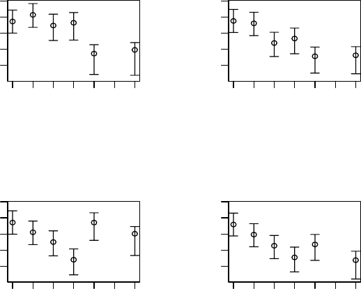
ment. Figure 6.4 shows the posterior means of the log innovation variances

for each treatment. Within each treatment, the innovation variances do not

show much structure as a function of time. However, there appear to be some

large diﬀerences across treatments. For example, the innovation variances for

the high dose at weeks4and6are considerably higher than for the other

three treatments. These plots suggest that the innovation variances at weeks

4and6couldbemodeled as a function of treatment.

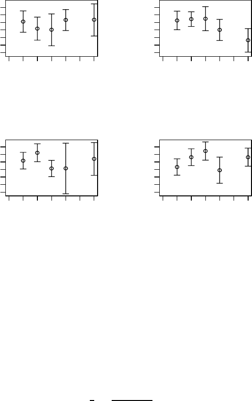
Figure 6.5 shows the lag-1 GARP for each treatment, again plotted as a

function of time. Here, the lag-1 GARP at week 6 for the medium dose is

much smaller than for the other three treatments (with its credible interval

not overlapping with the standard dose treatment) and we could allow this

GARP to diﬀer by treatment.

This exploratory analysis suggests the covariance matrix for the schizophre-

nia data does depend on treatment, and the GARP/IV parameterization pro-

vides a parsimonious way to model this as the individual parameters can de-

pend (or not) on (a subset of) treatment groups and the resulting covariance

matrices will be guaranteed to be positive deﬁnite.

These GARP/IV models will be explored more formally for the Growth

Hormone data in Chapter 7. For a detailed application of these models, see

Pourahmadi and Daniels (2002).

The modiﬁed Cholesky parameterization has also been used to introduce

covariates into the random eﬀects covariance matrix in the normal random

eﬀects model (Example 2.1) (Daniels and Zhao, 2003) and could also be used

for the random eﬀects covariance matrixingeneralized linear mixed models

(Example 2.2); however, there should be some implicit or explicit ordering of

the random eﬀects for this parameterization to be fully justiﬁed because the

parameterization is not invariant to the ordering of the components of b

.Ifthe

components of b

were the coeﬃcients of orthogonal polynomials or regression

splines, there is an obvious ordering. For a detailed example of introducing

132 INFERENCE UNDER MAR

0123456

3.5 4.5 5.5

(a)

Weeks

Log(IV)

0123456

3.5 4.5 5.5

(b)

Weeks

Log(IV)

0123456

3.5 4.5 5.5

(c)

Weeks

Log(IV)

0123456

3.5 4.5 5.5

(d)

Weeks

Log(IV)

Figure 6.4 Schizophrenia trial: posterior means of log of the innovation variances

(as a function of week) with 95% credible intervals for each treatment: (a) low dose,

(b) medium dose, (c) high dose, (d) standard treatment.

covariates into the random eﬀects matrix, we refer the reader to Daniels and

Zhao (2003). In Section 7.3, we allow the random eﬀects covariance matrix in

the schizophrenia trial to diﬀer by treatment.

There are other less computationally friendly ways to introduce covari-

ates into a covariance/correlation matrix. In the setting of the multivari-

ate normal model, there has been work on modeling the logarithm of the

marginal variances while keeping the correlation matrix constant across co-

variates (Manly and Rayner, 1987; Barnard, McCulloch, and Meng, 2000;

Pourahmadi, Daniels, and Park, 2007).

COVARIATE-DEPENDENT STRUCTURES 133

0123456

0.0 0.6 1.2

(a)

Weeks

GARP

0123456

0.0 0.6 1.2

(b)

Weeks

GARP

0123456

0.0 0.6 1.2

(c)

Weeks

GARP

0123456

0.0 0.6 1.2

(d)

Weeks

GARP

Figure 6.5 Schizophrenia trial: posterior means of lag-1 GARP (as a function of

week) with 95% credible intervals for each treatment: (a) low dose, (b) medium dose,

Modeling the correlation matrix as a function of covariates in the

multivariate probit model

In the setting of multivariate probit models, we can model the individual

correlations as a function of covariates. The typical approach is to individually

transform the correlations to R using Fisher’s z-transform

z(ρ

ijk

log

(1 − ρ

ijk

)

(1 + ρ

ijk

)

= v

ijk

(Czado, 2000). This transformation of the individual correlations does not

guarantee the resulting correlation matrices are positive deﬁnite. Hence, the

vector of regression coeﬃcients for the correlations γ will be constrained;

within a Gibbs sampling algorithm, values of γ sampled corresponding to a

134 INFERENCE UNDER MAR

non-positive deﬁnite correlation matrix will have prior probability zero and

will be rejected within a Metropolis-Hastings algorithm.

Modeling the covariance function in terms of covariates

For temporally misaligned data, similar approaches can be applied to co-

variance/correlation functions. Consider theexponential covariance function

introduced in Example 2.4,

C(t

; σ

,φ)=σ

exp(−φ|t

− t

|).

Anatural way to introduce covariates here is through log(σ

)andlog(φ)

(assuming φ>0) as these transformations provide a set of unconstrained

parameters to maintain positive deﬁniteness of C(·, ·; σ

,φ).

6.5.2 Dependence in longitudinal binary models

Forlongitudinal binary data models based on underlying normal latent vari-

ables (Example 2.6) or random eﬀects (Example 2.2), covariates can be intro-

duced into their corresponding correlation/covariance matrix as discussed in

the previous section. For (marginalized)transition models, covariates can be

introduced through the (unconstrained) Markov dependence parameters.

Recall a marginalized transition model of order one (MTM(1)) has (Markov)

dependence parameters γ

, j =2,...,J.Theγ

are (unconstrained) log odds

ratios that can be modeled as a function of covariates via

= v

α,

with few additional computations compared to models without covariates. For

higher-order MTMs, the dependence parameters corresponding to lags larger

than one also are unconstrained and can be similarly modeled.

These models are ﬁt to data from the CTQ I trial in Section 7.4.

6.6 Joint models for multivariate processes

Multiple longitudinal processes are typically modeled separately, despite po-

tential gains in eﬃciency from modeling them jointly, unless there is inter-

est speciﬁcally in the relationship between the multiple processes (Liu and

Daniels, 2007). In the case of incomplete data, there are additional reasons

to build and base inference on joint models. Joint modeling allows the use of

all available data, on both the process of interest and the other processes, to

‘impute’ the missing values on the processofinterest. This can be especially

advantageous when (1) the processes are not all observed at the same times

and observed responses for other processes are ‘closer’ temporally than ob-

served responses from the same processand(2)the correlation between the

JOINT MODELS FOR MULTIVARIATE PROCESSES 135

processes is strong. By modeling the processes separately, we do not use the

information from the other processes to ﬁll in the missing values.

Our primary interest here in developing joint models will be to incorporate

auxiliary variables under the auxiliary variable MAR (A-MAR) assumption

(Deﬁnition 5.11), where missingness in Y is MAR after conditioning on the

observed responses y

obs

,modelcovariates X, and auxiliary covariates V .Let

obs

be the observed values of the auxiliary covariate process. Then A-MAR

corresponds to the following form of the missing data mechanism,

p(r | y, x, v

obs

)=p(r | y

obs

, x, v

obs

In Bayesian inference, to allow for A-MAR mechanisms, we need to specify

the joint distribution p(y, v | x)andthenintegrate out v

p(y | x)=



p(y, v | x)dv (6.15)

to obtain the full data response model of interest; from a practical perspective,

joint models for which this integral can be obtained in closed form would be

preferred. When the auxiliary covariate(s) are time-varying, joint longitudinal

models can be constructed for the auxiliary process V and the process of

interest Y .

For the CTQ II example (Section 1.4), the A-MAR assumption implies

that probability of missingness of cessation status at time t is independent of

the unobserved cessation status at time t conditional on the previous weeks’

smoking responses and the previous weeks’ weight change responses (as op-

posed to conditional on just the previous weeks’ smoking responses). In a data

augmentation step, we draw Y

mis

from p(y

mis

| y

obs

, v

obs

), not p(y

mis

| y

obs

Hence, the A-MAR assumption is weaker than MAR to the extent that we can

correctly specify the distribution p(y, v | x). In the following, we review and

introduce some models for multivariate processes that are convenient when

one of the processes is of primary interest and the other process is an aux-

iliary covariate process (Carey and Rosner, 2001; Gueorgeiva and Agresti,

2001; O’Brien and Dunson, 2004; Liu and Daniels, 2007). In particular, the

models presented here lend themselves to the setting of auxiliary time-varying

covariates in that the full data responsemodelofinterestcan be obtained in

closed form (cf. (6.15)). We ﬁt one of these models to the CTQ II smoking

cessation data in Section 7.5.

In the following examples, we denote Y

as the primary response of interest

and V

as the auxiliary covariate process at time t

6.6.1 Continuous response and continuous auxiliary covariate

As a starting point, we assume both processes are (potentially) measured at

the same set of observation times (t

= t

). For continuous data, the multi-

variate normal distribution is an obvious choice for the joint distribution of the

136 INFERENCE UNDER MAR

longitudinal processes. We model the joint distribution of the two processes,

, V

), as

∼ N (x

β, Σ),

where

Σ =

The extension of this model to more than one auxiliary covariate process is

obvious. The dimension of Σ can be quite large, so structure is often imposed

on Σ using latent variables (Roy and Lin, 2000) or by inducing structure

directly on Σ (Carey and Rosner, 2001). To illustrate, consider models for

CD4 where the auxiliary covariate is viral load.

Consider the following (serial correlation) structure for Σ (Carey and Ros-

ner, 2001),

cov(Y



)=σ

−t



cov(V



)=σ

−t



cov(Y



)=σ

−t



+1|

The ﬁrst two covariances correspond to within-process covariances for the

primary response (CD4) and the auxiliary covariate (viral load), and the third

corresponds to the between-process covariance. For each, it is assumed that

the correlation decreasesforresponses farther apart in time by restricting γ

,andγ

to be in [0, 1). The parameter γ

determines the relationship

between CD4 and viral load; if γ

=0,thenthey are independent processes.

Missing data is imputed in the data augmentation step by constructing

the appropriate conditional distributions from this multivariate normal model

with a structured covariance matrix. Clearly, this form of Σ implies that

observed responses closer in time tothemissing responses will carry more

weight in the imputation and the magnitude of γ

will determine how much

information is used from the auxiliary covariates process to ﬁll in values for

the primary process.

Multivariate normal models are natural for handling time-varying continu-

ous(auxiliary) covariates as the conditional distribution of one process given

the other can be written downinclosedform(asalinearregression)aswell

as the marginal distribution of the primary process of interest using standard

multivariate normal results.

JOINT MODELS FOR MULTIVARIATE PROCESSES 137

The covariance structures described here also can be used for misaligned

measurement times by inducing a structured covariance function within a

Gaussian process.

6.6.2 Binary response and binary auxiliary covariate

Models for a binary response and binary auxiliary covariate can be speciﬁed

similarly to those described in Section 6.6.1. Let Y

= I{Z

> 0} and V

I{Z

> 0} where Z

=(Z

,...,Z

)

and Z

=(Z

,...,Z

)

are latent

variables modeled as

∼ N (x

β, Σ)

with

Σ =

The covariance matrix Σ is a correlation matrix for identiﬁability (cf. the

multivariate probit model in Example 2.6). Models using latent normal for-

mulations are convenient for speciﬁcation of dependence and computations.

Recent work has also considered allowing the latent variables to follow a

multivariate t-distribution (O’Brien and Dunson, 2004). One reason for using

a t-distribution is that when the scale matrix and degrees of freedom are appro-

priately speciﬁed, the multivariate t-distribution approximates a multivariate

logistic model; that is, the marginal distribution of Z

follows (approximately)

alogistic distribution, which in turn implies P (Y

ijk

=1| x

)follows a logistic

regression model. Computations are as easy as the probit model given that

the multivariate t-distribution can be re-expressed as a gamma mixture of

multivariate normals (see Example 3.16).

Similar to the model described in Section 6.6.1, this class of models is well-

suited for handling time-varying auxiliary covariates as the conditional and

marginal distributions of the process of interest take a simple form due to the

underlying normal (or t-) latent structure.

We ﬁnish our discussion of joint modeling in the next section by introducing

amodel for a binary primary process of interest and a continuous auxiliary

covariate (or vice versa). This is motivated by the CTQ II smoking cessation

data (Section 1.4) where the primary process of interest was smoking cessation

(binary) and the auxiliary covariate was weight change (continuous).

138 INFERENCE UNDER MAR

6.6.3 Binary response and continuous auxiliary covariate

Astraightforward way to induce correlation between a continuous and a bi-

nary longitudinal process is to specify a joint multivariate normal distribution

for the continuous responses and the latent variables underlying the binary

process, with the restriction that the marginal covariance matrix correspond-

ing to the binary responses is a correlation matrix. This model has appeared

in various forms in the literature (Catalano and Ryan, 1992; Gueorgeiva and

Agresti, 2001; Liu and Daniels, 2007).

As in Section 6.6.2, Y

= I{Z

> 0} where Z is the vector of latent

variables underlying the vector of longitudinal binary responses Y ,and(Z, V )

are jointly multivariate normal as follows:

∼ N (x

β, Σ),

where, as above,

Σ =

with Σ

acorrelation matrix. Notice that the marginal distribution of Z

multivariate normal and the marginal distribution of Y

follows a multivari-

ate probit model.Thesubmatrix Σ

characterizes the dependence between

the continuous and binary longitudinal processes. If Σ

= 0,thenthe two

longitudinal processes are independent.

This model is used to address an auxiliary covariate (process) in the CTQ II

smoking cessation data in Section 7.5.

6.7 Model selection and model ﬁt under ignorability

We now propose some modiﬁcations of the techniques for model comparison

and for assessing model ﬁt, ﬁrst introduced in Chapter 3, that can be extended

to incomplete data settings (under ignorability). Before we discuss these mod-

iﬁcations, we remind the reader that we can only assess the ﬁt of the full-data

model to the observed data;theadequacy of the model for the missing data

cannot be ascertained. Diﬀerent full-data models that provide the same ﬁt to

the observed data should be indistinguishable when using sensible model se-

lection criteria even though they may make very diﬀerent assumptions about

the missing data.

Because the focus of this chapter has been on ignorable missingness, we

MODEL SELECTION AND MODEL FIT 139

assess the ﬁt of the model using only the full-data response model p(y | θ),

and not the full data model p(y, r | ω)because it was unnecessary to specify

p(r | y

obs

, ψ). For nonignorable mechanisms, we do need to use p(y, r | ω);

this will be presented in detail in Chapter 8.

6.7.1 Deviance information criterion (DIC)

With complete data, the DIC is constructed using the likelihood based on the

full-data response model. The complication in using the DIC with incomplete

data under ignorability is that we do not observe the full data. The literature

is sparse on recommendations for constructing the DIC from incomplete data.

We consider two constructions based on those used in Pourahmadi and Daniels

(2002), Ilk and Daniels (2007) and Celeux et al. (2007). The recommendations

in Celeux et al., however, may not generalize well to our setting as they deal

with missing data that are latent (e.g., in the context of mixture and random

eﬀects models). Latent data are of course fundamentally diﬀerent than missing

response data. First, we can never observe the latent data, but we could have

observed the missing response data. Second, the observed vector of missingness

indicators has no analog in random eﬀects and mixture models.

DIC based on the observed data likelihood

Aﬁrst,andperhaps most obvious construction based on the development

in Chapter 5 and Section 6.1 would betoconstructtheDICbasedonthe

observed data likelihood L(θ | y

obs

DIC

=DIC

obs

)=−4E{ (θ | y

obs

)} +2(θ | y

obs

where

θ = E(θ | y

obs

). This approach has been applied by Pourahmadi and

Daniels (2002) and Ilk and Daniels (2007) and typically can be computed

directly in WinBUGS.

DIC based on the full-data likelihood

An alternative approach would be to constructtheDICbased on the full-data

response model likelihood,

DIC

full

obs

, y

mis

)=−4E

{(θ | y

obs

, y

mis

)} +2{θ(y

mis

) | y

obs

, y

mis

where E

(·)istheexpectation with respect to p(θ | y)and

θ(y

mis

E(θ | y

obs

, y

mis

). Since y

mis

is not observed, we take the expectation of

DIC

full

obs

, y

mis

)withrespect to the posterior predictive distribution p(y

mis