Daniels M.J., Hogan J.W. Missing Data in Longitudinal Studies: Strategies for Bayesian Modeling and Sensitivity Analysis

Подождите немного. Документ загружается.

120 INFERENCE UNDER MAR

the posterior for the mean parameters in Bayesian inference replaces (β, α)

in (6.8) with (β, α)+logp(β, α). 2

We illustrate using a multivariate normal model.

Example 6.2. Information matrix based on observed data log likelihood un-

der ignorability with a multivariate normal model.

Assume Y

follows a multivariate normal distribution with mean X

β and

covariance matrix Σ(α). Let θ =(β, α)andassume that p(β, α)=p(β)p(α)

(a common assumption). For the case of complete data, it is easy to show

that the oﬀ-diagonal block of the information matrix, I

β,α

,isequalto zero

for all values of α,therebysatisfying condition (6.8). For Bayesian inference,

the posterior for β will be consistent even under mis-speciﬁcation of Σ(α).

However, under ignorability, the submatrix of the information matrix, now

based on the observed data log likelihood 

obs

(or observed dataposterior)

and given by

obs

β,α

(β, α)=− E



∂



obs

(β, α)

∂β∂α



is no longer equal to zero even at the true value for Σ(α)(Little and Rubin,

2002). Hence the weaker parameter orthogonality condition given in Deﬁnition

6.2 does not even hold. As a result, in order for the posterior distribution of the

mean parameters to be consistent, the dependence structure must be correctly

speciﬁed.

This lack of orthogonality can be seen in the setting of a bivariate normal

linear regression, by making a simple analogy to univariate simple linear re-

gression. This will also provide some additional intuition into how inferences

change under missingness.

Suppose E(Y )=µ, R

=1fori =1,...,n

observed), and R

=0for

i = n

+1,...,n(y

missing). As in Chapter 5, we factor the joint distribution

of p(y

)asp(y

)p(y

| y

). For complete data, the conditional distribution

of Y

given Y

(ignoring priors for the time being) as a function of µ

and

= σ

/σ

is proportional to

exp

−



i=1

− µ

− φ

− µ

)}

/2σ

2|1

, (6.9)

where σ

2|1

= σ

− σ

−1

.Notethatφ

and µ

do not appear in p(y

Theorthogonality of µ

and φ

is apparent by recognizing (6.9) as the

same form as the log likelihood for a simple linear regression having a centered

covariate y

− µ

with intercept µ

and slope φ

.Itcanbeshownfromthis

form that the element of the (expected) information matrix corresponding to

and φ

is zero for all values of φ

.However, with missing data (under

DATA AUGMENTATION 121

MAR), the analogue of (6.9) is

exp

−



i=1

− µ

− φ

− µ

)}

/2σ

2|1

The sum is now only over the terms that correspond to R

=1.

Recall the mean of the completers at time j is µ

= E(Y

| R =1).Again

using the analogy to simple linear regression, µ

and φ

are orthogonal,

but µ

and φ

arenot.This is clear from the following, which holds under

ignorability:

= µ

π + µ

(1 − π)

= µ

− φ

(1 − π)(µ

− µ

where π = P (R

=1).Thus,µ

is a function of φ

.Withnomissing data,

π =1(soµ

= µ

). Under MCAR, (µ

− µ

)=0andthesecond term

involving φ

disappears. 2

Examples 6.1 and 6.2 demonstrate the importance of correctly specifying

Σ even when primary interest is in µ.Thus,ifwemodel the covariance matrix

parsimoniously, we must be sure to consider whether Σ depends on covariates.

Of course, such modeling decisionsareonlyveriﬁable from the data underthe

ignorability assumption.

Similar results hold for directly speciﬁed models for binary data. It can

be shown that the information matrix for the mean parameters β and the

dependence parameters α in an MTM(1) (Example 2.5) satisﬁes condition

(6.8) under no missing data or MCAR (Heagerty, 2002) , but not under MAR.

There are also situations where misspeciﬁcation of dependence with com-

plete data can lead to biased estimates of the mean parameters. For example,

in marginalized transition model of order p (where p ≥ 2), β and α are not

orthogonal (Heagerty, 2002). Hence, the dependence structure must be cor-

rectly speciﬁed. Similar speciﬁcationissues with complete data are also seen

in conditionally speciﬁed models for binary data.

Of course, it is not possible to verify whether the dependence structure is

correct when data are incomplete. As a practical matter, when ignorability

is being assumed, it is recommended that the dependence model be selected

based on the model that is most suitable for the observed data.

6.3 Posterior sampling using data augmentation

Data augmentation is an important tool for full data inference in the pres-

ence of missing data; it is related to theEMalgorithm (Dempster, Laird, and

Rubin, 1977) and its variations (van Dyk and Meng, 2001). As we illustrated

in Chapter 5 the general strategy is to specify a model and priors for the full

data and then to base posterior inference on the induced observed data pos-

122 INFERENCE UNDER MAR

terior, p(θ | y

obs

). However, the full-data posterior p(θ | y)isofteneasier to

sample than the observed-data posterior p(θ | y

obs

). Speciﬁcally, full condi-

tional distributions of the full-data posterior used in Gibbs sampling typically

have simpler forms than the full conditionals derived using the observed-data

posterior. This motivates augmenting the observed-data posterior with the

missing data y

mis

.Wepointout that if the model is speciﬁed directly for the

observed data, i.e, specify the observed data response model instead of the

full-data response model, and priors are put directly on the parameters of the

observed-data response model (see Example 5.7), then data augmentation is

not needed.

For data augmentation, at each iteration k of the sampling algorithm, we

sample (y

(k)

mis

, θ

(k)

)via

1. y

(k)

mis

∼ p(y

mis

| y

obs

, θ

(k−1)

)

2. θ

(k)

∼ p(θ | y

obs

, y

(k)

mis

Thus, we can sample θ using the tools we described in Chapter 3 for the full-

data posterior, as if we had complete data. Implicitly, via Monte Carlo integra-

tion within the MCMC algorithm, we obtain a sample from the observed-data

posterior p(θ | y

obs

)givenin (6.3).

Because data augmentation depends on sampling from p(y

mis

| y

obs

, θ), the

augmentation depends heavily on the within-subject dependence structure.

We illustrate by giving some examples of the data augmentation step for

several models from Chapter 2 under ignorable dropout.

Example 6.3. Data augmentation under ignorability with a multivariate nor-

mal model (continuation ofExample2.3).

Without loss of generality, deﬁne Y

obs,i

=(Y

,...,Y



)

and Y

mis,i

i,J



,...,Y

)

with corresponding partitions of X

and Σ given by

obs,i

mis,i

Σ =

obs

obs,mis

mis

Within the sampling algorithm, the distribution of p(y

mis,i

| y

obs,i

, θ)takes

the form

mis,i

| Y

obs,i

, θ ∼ N(µ



, Σ



where



= x

mis,i

β + B(Σ)(y

obs,i

− x

obs,i

β)



= Σ

mis

− Σ

obs,mis

−1

obs

obs,mis

and B(Σ)=Σ

obs,mis

−1

obs

.Thedependence of Y

mis,i

on Y

obs,i

is governed

DATA AUGMENTATION 123

by B(Σ), the matrix of autoregressive coeﬃcients from regressing Y

mis,i

obs,i

.Clearly, B(Σ)isafunction of the full-data covariance matrix Σ. 2

Example 6.4. Data augmentation under ignorability with random eﬀects lo-

gistic regression (continuation ofExample2.2).

Again, we deﬁne Y

mis,i

and Y

obs,i

as in Example 6.3. The distribution p(y

mis,i

obs,i

, b

, θ)isaproduct of independent Bernoullis with probabilities

P (Y

mis,ij

=1| y

obs,i

, b

, θ)=

exp(x

β + w

)

1+exp(x

β + w

)

,j≥ J



+1. (6.10)

The dependence of these imputed values on the random eﬀects covariance

matrix Ω is evidenced by the presence of b

in (6.10). By integrating out b

(as in Example 2.2), we have

p(y

mis,i

| y

obs,i

, θ)=



p(y

mis,i

| y

obs,i

, b

, θ) p(b

| θ, y

obs,i

) db



p(y

mis,i

| b

, β) p(b

| β, Ω, y

obs,i

) db

. (6.11)

The integral (6.11) is not available in closed form; however, recalling that the

population-averaged distribution can be approximated by

P (Y

mis,ij

=1| y

obs,i

, θ) ≈

exp(x



)

1+exp(x



)

where β



≈ βK(Ω)andK(Ω)isaconstantthat depends on Ω,thedepen-

dence on the random eﬀects covariance matrix is clear. 2

Data augmentation and multiple imputation

Certain types of multiple imputation (Rubin, 1987) can be viewed as ap-

proximations to data augmentation. Bayesianly proper multiple imputation

(Schafer, 1997) provides an approximation to the fully Bayesian data augmen-

tation procedure in (6.3), which is based on the full-data response model; for

nonignorable missingness (Chapter 8), it would be based on the entire full-

data model. This approximation is computed by sampling just a few values,

say M ,fromp(y

mis

| y

obs

)(asopposed to full Monte Carlo integration). The

M sets of y

mis

are then usedtocreateM full datasets that are analyzed using

full-data response log likelihoods, (θ | y)orfull-data response model poste-

riors p(θ | y). Inferences are then appropriately adjusted for the uncertainty

in themissing values (Schafer, 1997).

Bayesianly ‘improper’ multiple imputation would sample M values from

some distribution, say p



mis

| y

obs

), where



mis

| y

obs

) = p(y

mis

| y

obs

This might be implemented when the imputation model is speciﬁed and ﬁt

124 INFERENCE UNDER MAR

separately from the full-data response model (Rubin, 1987) or when auxiliary

covariates V arebeing used under an MAR assumption.

6.4 Covariance structures for univariate longitudinal processes

In Examples 6.1 and 6.2, we showed the importance of covariance speciﬁca-

tion in incomplete data. We now describe a number of speciﬁc approaches to

accomplish this. For multivariate normal models where the dimension of Y

is large relative to the sample size, it is common to assume a parsimonious

structure for Σ to avoid having to estimate a large numberofparameters.

We discuss two classes of models that are computationally convenient to do

this. For the ﬁrst class, we directly specify the covariance structure. For the

second, we specify the covariance structure indirectly via random eﬀects.

6.4.1 Serial correlation models

Anatural parameterization on whichtointroduce structure for Σ in multivari-

ate normal models is via the parameters in the modiﬁed Cholesky decomposi-

tion (Pourahmadi, 1999). The parameters of this decomposition correspond to

the means and variances of the conditional distributions p(y

| y

,...,y

j−1

j =1,...,J,

E(Y

| y

,...,y

j−1

)=µ

j−1



k=1

− µ

), (6.12)

var(Y

| y

,...,y

j−1

)=σ

. (6.13)

The autoregressive coeﬃcients in (6.12),

{φ

: k =1,...,j− 1; j =2,...,J},

are called generalized autoregressive parameters (GARP) and characterize the

dependence structure. The variance parameters in (6.13),

{σ

: j =1,...,J} ,

are called the innovation variances (IV). A major advantage of these param-

eters is that the GARP are unconstrained regression coeﬃcients and the logs

of the innovation variances are also unconstrained, unlike the variance and

covariances {σ

} of Σ.

The GARP/IV parameters are also natural for characterizing missingness

due to dropout and for characterizing identifying restrictions given their con-

nections to the conditional distributions p(y

| y

,...,y

j−1

). This was brieﬂy

discussed in Example 5.11 and will be discussed in detail in Section 8.4.2 in

Chapter 8.

Before discussing a particular class of models based on the GARP and IV

COVARIANCE STRUCTURES 125

parameters, we review some approaches to explore the feasibility of diﬀerent

parsimonious structures based on these parameters.

Exploratory analysis of GARP/IV parameters

Exploratory model selection can be conducted by examining an unstructured

estimate of Σ and by examining regressograms (Pourahmadi, 1999), which

plot the GARP and IV parameters vs. both lag and time. We illustrate both

these approaches on the schizophrenia data (Section 1.2). To simplify this

demonstration, we ignore the fact that the lag between the last two measure-

ments was 2 weeks, not 1 week.

Table 6.1 Schizophrenia trial: GARP parameters from ﬁtting a multivariate normal

model. The elements in the matrix are φ

j,j+k

Week (j)

Lag (k)1 2 3 4 5

1.81.89.85 .68 .80

2–.07.03.30 .14

3.17–.10 .06

4–.02.03

5–.04

Table 6.1 showstheestimated GARP parameters from ﬁtting a multivari-

ate normal model to the schizophrenia data. The lag-1 parameters (ﬁrst row)

are the largest and appear to characterize most of the dependence. We can also

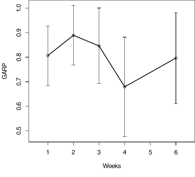
view the GARP graphically using regressograms. Figure 6.1 shows a regresso-

gram of the lag-1 GARP as a function of week (corresponding to the ﬁrst row

of Table 6.1); there is little structure to exploit here other than potentially

assuming the lag-1 GARP are constant over week φ

j,j+1

= φ

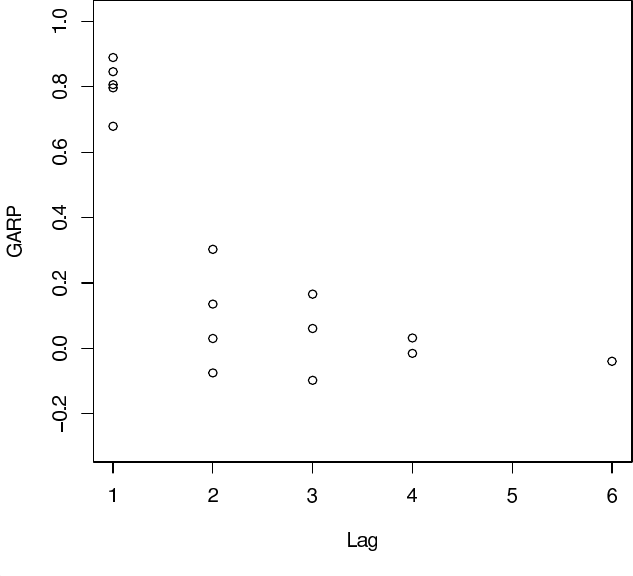
Figure 6.2 is another regressogram showing the GARP as a function of lag

(for example, the ﬁrst column in the ﬁgure has a dot for each of the ﬁve lag-1

GARP given inTable6.1). The GARP for lags greater than 2 seem small,

suggesting these parameters can be ﬁxed at zero. An alternative approach,

as suggested in Pourahmadi (1999) would be to model the GARP using a

polynomial in lag. Based on Figure 6.2, a quadratic might be adequate for

this data and would reduce the number of GARP parameters from ﬁfteen to

three. Note that this model implicitly assumes that for a given lag, the GARP

are constant.

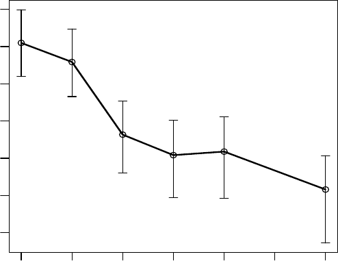
Figure 6.3 shows the log of the IV as a function of weeks. Clearly, the

126 INFERENCE UNDER MAR

Figure 6.1 Schizophrenia trial: posterior means of lag-1 GARP with 95% credible

intervals as a function of weeks.

innovation variances are decreasing over time andasimplelinear trend in

weeks would likely be adequate to model the IV, reducing the number of IV

parameters from six to two.

Structured GARP/IV models for Σ

Structured GARP/IV models (Pourahmadi and Daniels, 2002) specify linear

and log-linear models for the GARP and IV parameters, respectively, via

= v

γ,k=1,...,j− 1; j =2,...,J

log(σ

)= d

λ,j=1,...,J. (6.14)

The design vector v

can be speciﬁed as a smooth function in lag (j − k)(cf.

Figure 6.2) and/or a smooth function in j foraﬁxedlagj − k (cf. Figure 6.1).

The design vector d

can be speciﬁed as a smooth function of j (cf. Figure

6.3). These smooth functions are typically chosen as low-order polynomials

COVARIANCE STRUCTURES 127

Figure 6.2 Schizophrenia trial: posterior means of GARP as a function of lag.

(or splines). Special cases of these models include setting φ

= φ



|j−k|

for all

j and k, i.e., constant within lag (stationary) GARP. A ﬁrst-order structure

would set φ



|j−k|

=0for|j − k| > 1.

Based on our exploratory analysis of the schizophrenia data, we might

specify a ﬁrst order lag structure for the GARP. As such, the design vector

for the GARP would be



1 |j − k| =1

0otherwise

with γ representing the lag-1 regression coeﬃcient. We might specify a linear

model for the log IV, setting d

=(1,j)

Apracticaladvantage of structured GARP/IV models is that they allow

simple computations since the GARP regression parameters γ have full con-

ditional distributions that are normal when the prior on γ is normal (see

Pourahmadi and Daniels, 2002). In general, ﬁtting these models in WinBUGS

128 INFERENCE UNDER MAR

0123456

3.8 4.0 4.2 4.4 4.6 4.8 5.0

Weeks

Log(IV)

Figure 6.3 Schizophrenia trial: posterior means of log of the IV as a function of

weeks.

can be diﬃcult (slow mixing) because WinBUGS does not recognize that

the full conditional distributions of the mean regression coeﬃcients and the

GARP regression parameters are both multivariate normal (see Pourahmadi

and Daniels, 2002). However, for some simple cases, these can be ﬁt eﬃciently

in WinBUGS. In Chapter 7, we explore models based on these parameters

further (including the computations) for the Growth Hormone trial (Section

1.3).

6.4.2 Covariance matrices induced by random eﬀects

Random eﬀects are another way to parsimoniously model the dependence

structure. Whereas the GARP/IV modelsparameterize the covariance matrix

directly, random eﬀects models induce structure on the covariance matrix

indirectly.

COVARIANCE STRUCTURES 129

Recall the normal random eﬀects model (Example 2.1),

| x

, b

∼ N(µ

, Σ

)

| Ω ∼ N (0, Ω),

with

= x

β + w

Here, we set Σ

= σ

I.Themarginalcovariance structure for Y

,afterinte-

grating out the random eﬀects, is

Σ = σ

I + w

Ωw

with j, k element

= σ

I(j = k)+w

Ωw

where w

is the jth row of w

and dim(Ω)=q.Thevector of covariance

parameters has dimension q(q +1)/2+1 whereasthevector of parameters of

an unstructured Σ has dimension J(J +1)/2. Typically, q  J.

For the schizophrenia clinical trial analysis in Chapter 7, we specify w

usinganorthogonal quadratic polynomial (q =3).Assuch,wereduce the

number of covariance parameters from 21 to 7.

The random eﬀects structure is an alternative to the GARP/IV struc-

ture and can also be used to introduce structured dependence in general-

ized linear mixed models (cf. Example 2.2). It is possible to combine struc-

tured GARP/IV models with random eﬀects by decomposing Σ as Σ = Σ

Ωw

and modeling Σ

using a parsimonious GARP/IV model (Pourah-

madi and Daniels, 2002).

6.4.3 Covariance functions for misaligned data

As discussed in Example 2.4, a structured covariance is typically required

to estimate the covariance function for misaligned temporal data. We review

some examples next.

For temp orally misaligned longitudinal data, the covariance structure is

typically summarized via a covariance function,

cov(Y

; φ)=C(t

; x

, φ).

To draw inference about this function, simplifying assumptions (about the

process) or structure (on the function itself) are necessary because it is often

the casethatno(orfew)replications are available for observations at certain

times or pairs of times. In the remaining development, we drop the dependence

on x in the covariance function for clarity.

Acommon assumption is (weak) stationarity, where the covariance func-

tion C(t

; φ)isonlyafunction of the diﬀerence between times, i.e.,