Daniel W.W. Biostatistics: A Foundation for Analysis in the Health Sciences

Подождите немного. Документ загружается.

9.3 THE SAMPLE REGRESSION EQUATION 417

FIGURE 9.3.2 MINITAB procedure and output for obtaining the least-squares regression

equation from the data in Table 9.3.1.

Dialog box: Session command:

Stat ➤ Regression ➤ Regression MTB > Name C3 = ‘FITS1’ C4 = ‘RESI1’

Type y in Response and x in Predictors. MTB > Regress ‘y’ 1 ‘x’;

Click Storage. Check Residuals and Fits. SUBC> Fits ‘FITS1’;

Click OK . SUBC> Constant;

SUBC> Residuals ‘RESI1’.

Output:

Regression Analysis: y versus x

The regression equation is

y = -216 + 3.46 x

Predictor Coef Stdev t-ratio p

Constant -215.98 21.80 -9.91 0.000

x 3.4589 0.2347 14.74 0.000

s = 33.06 R-sq = 67.0% R-sq(adj) = 66.7%

Analysis of Variance

SOURCE DF SS MS F p

Regression 1 237549 237549 217.28 0.000

Error 107 116982 1093

Total 108 354531

Unusual Observations

Obs. x y Fit Stdev.Fit Residual St.Resid

58 86 155.00 82.52 3.43 72.48 2.20R

65 120 90.41 197.70 7.23 -107.29 -3.33R

66 120 106.00 198.74 7.29 -92.74 -2.88R

71 107 87.99 154.12 4.75 -66.13 -2.02R

97 106 241.00 150.66 4.58 90.34 2.76R

102 109 229.00 161.38 5.13 67.62 2.07R

103 115 253.00 181.79 6.28 71.21 2.19R

R denotes an obs. with a large st. resid.

From Figure 9.3.2 we see that the linear equation for the least-squares line that

describes the relationship between waist circumference and deep abdominal AT may be

written, then, as

This equation tells us that since is negative, the line crosses the Y-axis below the

origin, and that since the slope, is positive, the line extends from the lower left-hand cor-

ner of the graph to the upper right-hand corner. We see further that for each unit increase

in x, y increases by an amount equal to 3.46. The symbol y denotes a value of y computed

from the equation, rather than an observed value of Y.

By substituting two convenient values of X into Equation 9.3.2, we may obtain the

necessary coordinates for drawing the line. Suppose, ﬁrst, we let and obtain

If we let we obtain

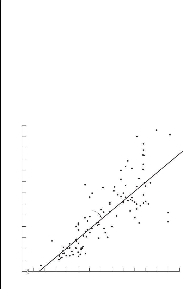
The line, along with the original data, is shown in Figure 9.3.3.

=-216 + 3.4611102= 164

X = 110

=-216 + 3.461702= 26.2

X = 70

=-216 + 3.46x

418

CHAPTER 9 SIMPLE LINEAR REGRESSION AND CORRELATION

Deep abdominal AT area (cm

), Y

Waist circumference (cm), X

100

120

140

160

180

200

220

240

260

60 65 70 75 80 85 90 95 100 105 110 115 120 125

216 + 3.46x

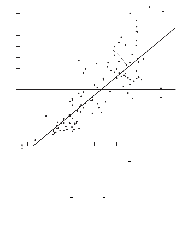
FIGURE 9.3.3 Original data and least-squares line for Example 9.3.1. ■

The Least-Squares Criterion Now that we have obtained what we call the

“best ﬁt” line for describing the relationship between our two variables, we need to deter-

mine by what criterion it is considered best. Before the criterion is stated, let us exam-

ine Figure 9.3.3. We note that generally the least-squares line does not pass through the

observed points that are plotted on the scatter diagram. In other words, most of the

observed points deviate from the line by varying amounts.

The line that we have drawn through the points is best in this sense:

The sum of the squared vertical deviations of the observed data points ()from the

least-squares line is smaller than the sum of the squared vertical deviations of the data

points from any other line.

In other words, if we square the vertical distance from each observed point ( )

to the least-squares line and add these squared values for all points, the resulting total

will be smaller than the similarly computed total for any other line that can be drawn

through the points. For this reason the line we have drawn is called the least-squares

line.

EXERCISES

9.3.1 Plot each of the following regression equations on graph paper and state whether X and Y are

directly or inversely related.

(a)

(b)

(c)

9.3.2 The following scores represent a nurse’s assessment (X ) and a physician’s assessment (Y ) of the

condition of 10 patients at time of admission to a trauma center.

X:181318151012 8473

Y:23201816141110764

(a) Construct a scatter diagram for these data.

(b) Plot the following regression equations on the scatter diagram and indicate which one you

think best ﬁts the data. State the reason for your choice.

(1)

(2)

(3)

For each of the following exercises (a) draw a scatter diagram and (b) obtain the regression

equation and plot it on the scatter diagram.

9.3.3 Methadone is often prescribed in the treatment of opioid addiction and chronic pain. Krantz et al.

(A-2) studied the relationship between dose of methadone and the corrected QT (QTc) interval for

17 subjects who developed torsade de pointes (ventricular tachycardia nearly always due to med-

ications). QTc is calculated from an electrocardiogram and is measured in mm/sec. A higher QTc

value indicates a higher risk of cardiovascular mortality. A question of interest is how well one

can predict and estimate the QTc value from a knowledge of methadone dose. This question is

typical of those that can be answered by means of regression analysis. Since QTc is the variable

= 1 + 1x

=-10 + 2x

= 8 + 0.5x

= 10 - 0.75x

= 3 + 0.5x

=-3 + 2x

EXERCISES 419

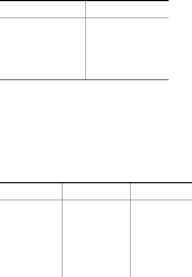
about which we wish to make predictions and estimations, it is the dependent variable. The

variable methadone dose, knowledge of which will be used to make the predictions and estima-

tions, is the independent variable.

Methadone Dose Methadone Dose

(mg/day) QTc (mm /sec) (mg/day) QTc (mm/sec)

1000 600 650 785

550 625 600 765

97 560 660 611

90 585 270 600

85 590 680 625

126 500 540 650

300 700 600 635

110 570 330 522

65 540

Source: Mori J. Krantz, Ilana B. Kutinsky, Alastair D. Roberston, and Philip

S. Mehler, “Dose-Related Effects of Methadone on QT Prolongation in a Series of

Patients with Torsade de Pointes,” Pharmacotherapy, 23 (2003), 802–805.

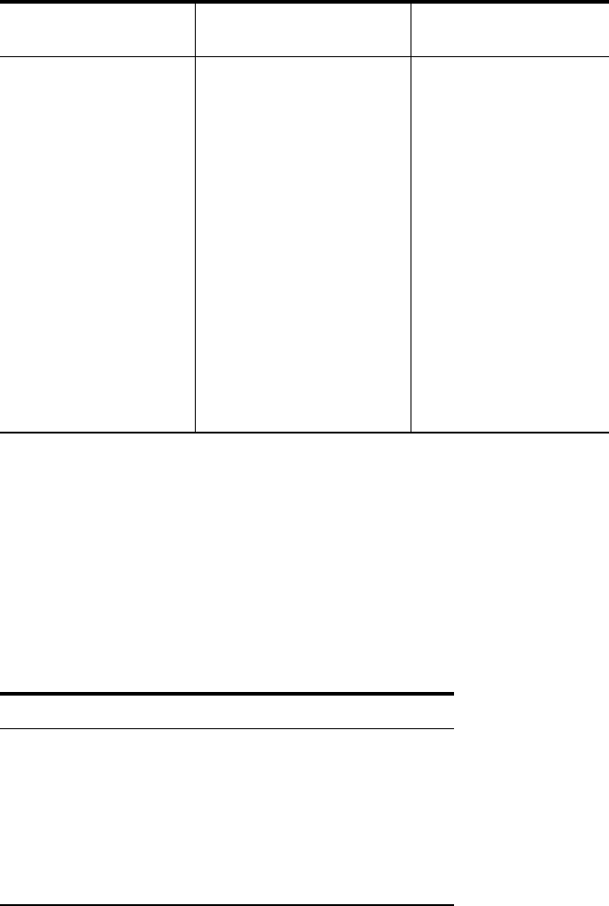
9.3.4 Reiss et al. (A-3) compared point-of-care and standard hospital laboratory assays for monitoring

patients receiving a single anticoagulant or a regimen consisting of a combination of anticoagulants.

It is quite common when comparing two measuring techniques, to use regression analysis in which

one variable is used to predict another. In the present study, the researchers obtained measures of

international normalized ratio (INR) by assay of capillary and venous blood samples collected from

90 subjects taking warfarin. INR, used especially when patients are receiving warfarin, measures the

clotting ability of the blood. Point-of-care testing for INR was conducted with the CoaguChek assay

product. Hospital testing was done with standard hospital laboratory assays. The authors used the

hospital assay INR level to predict the CoaguChek INR level. The measurements are given in the

following table.

CoaguChek Hospital CoaguChek Hospital CoaguChek Hospital

(Y)(X)(Y)(X)(Y)(X)

1.8 1.6 2.4 1.2 3.1 2.4

1.6 1.9 2.3 2.3 1.7 1.8

2.5 2.8 2.0 1.6 1.8 1.6

1.9 2.4 3.3 3.8 1.9 1.7

1.3 1.5 1.9 1.6 5.3 4.2

2.3 1.8 1.8 1.5 1.6 1.6

1.2 1.3 2.8 1.8 1.6 1.4

2.3 2.4 2.5 1.5 3.3 3.3

2.0 2.1 0.8 1.0 1.5 1.5

1.5 1.5 1.3 1.2 2.2 2.8

2.1 2.4 3.7 1.4 1.1 1.6

1.5 1.5 2.4 1.6 2.6 2.6

420 CHAPTER 9 SIMPLE LINEAR REGRESSION AND CORRELATION

(Continued)

CoaguChek Hospital CoaguChek Hospital CoaguChek Hospital

(Y)(X)(Y)(X)(Y)(X)

1.5 1.7 4.1 3.2 6.4 5.0

1.8 2.1 2.4 1.2 1.5 1.4

1.0 1.2 2.3 2.3 3.0 2.8

2.1 1.9 3.1 1.6 2.6 2.3

1.6 1.6 1.5 1.4 1.2 1.2

1.7 1.6 3.6 2.1 2.1 1.9

2.0 1.9 2.5 1.7 1.1 1.1

1.8 1.6 2.1 1.7 1.0 1.0

1.3 4.1 1.8 1.2 1.4 1.5

1.5 1.9 1.5 1.3 1.7 1.3

3.6 2.1 2.5 1.1 1.2 1.1

2.4 2.2 1.5 1.2 2.5 2.4

2.2 2.3 1.5 1.1 1.2 1.3

2.7 2.2 1.6 1.2 2.5 2.9

2.9 3.1 1.4 1.4 1.9 1.7

2.0 2.2 4.0 2.3 1.8 1.7

1.0 1.2 2.0 1.2 1.2 1.1

2.4 2.6 2.5 1.5 1.3 1.1

Source: Curtis E. Haas, Pharm.D. Used with permission.

9.3.5 Digoxin is a drug often prescribed to treat heart ailments. The purpose of a study by Parker et al. (A-4)

was to examine the interactions of digoxin with common grapefruit juice. In one experiment, subjects

took digoxin with water for 2 weeks, followed by a 2-week period during which digoxin was with-

held. During the next 2 weeks subjects took digoxin with grapefruit juice. For seven subjects, the

average peak plasma digoxin concentration (Cmax) when taking water is given in the ﬁrst column of

the following table. The second column contains the percent change in Cmax concentration when

subjects were taking the digoxin with grapefruit juice [GFJ (%) change]. Use the Cmax level when

taking digoxin with water to predict the percent change in Cmax concentration when taking digoxin

with grapefruit juice.

Cmax (ngl/ml) with Water Change in Cmax with GFJ (%)

2.34 29.5

2.46 40.7

1.87 5.3

3.09 23.3

5.59 45.1

4.05 35.3

6.21 44.6

2.34 29.5

Source: Robert B. Parker, Pharm.D. Used with permission.

9.3.6 Evans et al. (A-5) examined the effect of velocity on ground reaction forces (GRF) in dogs with

lameness from a torn cranial cruciate ligament. The dogs were walked and trotted over a force

EXERCISES 421

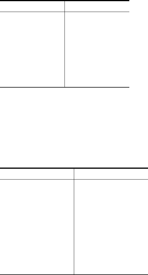
platform and the GRF recorded (in newtons) during the stance phase. The following table contains

22 measurements of force expressed as the mean of ﬁve force measurements per dog when walk-

ing and the mean of ﬁve force measurements per dog when trotting. Use the GRF value when

walking to predict the GRF value when trotting.

GRF-Walk GRF-Trot GRF-Walk GRF-Trot

31.5 50.8 24.9 30.2

33.3 43.2 33.6 46.3

32.3 44.8 30.7 41.8

28.8 39.5 27.2 32.4

38.3 44.0 44.0 65.8

36.9 60.1 28.2 32.2

14.6 11.1 24.3 29.5

27.0 32.3 31.6 38.7

32.8 41.3 29.9 42.0

27.4 38.2 34.3 37.6

31.5 50.8 24.9 30.2

Source: Richard Evans, Ph.D. Used with permission.

9.3.7 Glomerular ﬁltration rate (GFR) is the most important parameter of renal function assessed in renal

transplant recipients. Although inulin clearance is regarded as the gold standard measure of GFR,

its use in clinical practice is limited. Krieser et al. (A-6) examined the relationship between the

inverse of Cystatin C (a cationic basic protein measured in mg/L) and inulin GFR as measured by

technetium radionuclide labeled diethylenetriamine penta-acetic acid) (DTPA GFR) clearance

(ml/min/1.73 ). The results of 27 tests are shown in the following table. Use DTPA GFR as the

predictor of inverse Cystatin C.

DTPA GFR 1/Cystatin C DTPA GFR 1/Cystatin C

18 0.213 42 0.485

21 0.265 42 0.427

21 0.446 43 0.562

23 0.203 43 0.463

27 0.369 48 0.549

27 0.568 48 0.538

30 0.382 51 0.571

32 0.383 55 0.546

32 0.274 58 0.402

32 0.424 60 0.592

36 0.308 62 0.541

37 0.498 67 0.568

41 0.398 68 0.800

88 0.667

Source: David Krieser, M.D. Used with permission.

422 CHAPTER 9 SIMPLE LINEAR REGRESSION AND CORRELATION

9.4 EVALUATING THE REGRESSION EQUATION

Once the regression equation has been obtained it must be evaluated to determine

whether it adequately describes the relationship between the two variables and whether

it can be used effectively for prediction and estimation purposes.

When Is Not Rejected If in the population the relationship

between X and Y is linear, , the slope of the line that describes this relationship, will

be either positive, negative, or zero. If is zero, sample data drawn from the popu-

lation will, in the long run, yield regression equations that are of little or no value for

prediction and estimation purposes. Furthermore, even though we assume that the rela-

tionship between X and Y is linear, it may be that the relationship could be described

better by some nonlinear model. When this is the case, sample data when fitted to a

linear model will tend to yield results compatible with a population slope of zero. Thus,

following a test in which the null hypothesis that equals zero is not rejected, we

may conclude (assuming that we have not made a type II error by accepting a false

null hypothesis) either (1) that although the relationship between X and Y may be lin-

ear it is not strong enough for X to be of much value in predicting and estimating Y,

or (2) that the relationship between X and Y is not linear; that is, some curvilinear

model provides a better fit to the data. Figure 9.4.1 shows the kinds of relationships

between X and Y in a population that may prevent rejection of the null hypothesis that

When Is Rejected Now let us consider the situations in a pop-

ulation that may lead to rejection of the null hypothesis that . Assuming that

we do not commit a type I error, rejection of the null hypothesis that may be

attributed to one of the following conditions in the population: (1) the relationship is

linear and of sufficient strength to justify the use of sample regression equations to

predict and estimate Y for given values of X; and (2) there is a good fit of the data

to a linear model, but some curvilinear model might provide an even better fit. Fig-

ure 9.4.2 illustrates the two population conditions that may lead to rejection of

Thus, we see that before using a sample regression equation to predict and esti-

mate, it is desirable to test We may do this either by using analysis of vari-

ance and the F statistic or by using the t statistic. We will illustrate both methods. Before

we do this, however, let us see how we may investigate the strength of the relationship

between X and Y.

The Coefﬁcient of Determination One way to evaluate the strength of

the regression equation is to compare the scatter of the points about the regression line

with the scatter about the mean of the sample values of Y. If we take the scatter dia-

gram for Example 9.3.1 and draw through the points a line that intersects the Y-axis at

and is parallel to the X-axis, we may obtain a visual impression of the relative mag-

nitudes of the scatter of the points about this line and the regression line. This has been

done in Figure 9.4.3.

: b

= 0.

: b

= 0.

= 0

: B

 0

= 0.

: B

 0

9.4 EVALUATING THE REGRESSION EQUATION 423

It appears rather obvious from Figure 9.4.3 that the scatter of the points about

the regression line is much less than the scatter about the line. We would not wish,

however, to decide on this basis alone that the equation is a useful one. The situation

may not be always this clear-cut, so that an objective measure of some sort would be

much more desirable. Such an objective measure, called the coefﬁcient of determina-

tion, is available.

The Total Deviation Before deﬁning the coefﬁcient of determination, let us justify

its use by examining the logic behind its computation. We begin by considering the point

corresponding to any observed value, and by measuring its vertical distance from the

line. We call this the total deviation and designate it .

The Explained Deviation If we measure the vertical distance from the regres-

sion line to the line, we obtain , which is called the explained deviation, since

it shows by how much the total deviation is reduced when the regression line is ﬁtted to

the points.

- y2y

- y2

424 CHAPTER 9 SIMPLE LINEAR REGRESSION AND CORRELATION

(a)

(b)

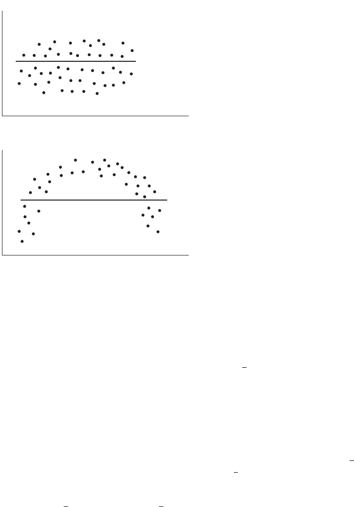
FIGURE 9.4.1 Conditions in a population that may prevent rejection of the null hypothe-

sis that (

) The relationship between

and

is linear, but is so close to zero that

sample data are not likely to yield equations that are useful for predicting

when

given. (

) The relationship between

and

is not linear; a curvilinear model provides a

better ﬁt to the data; sample data are not likely to yield equations that are useful for pre-

dicting

when

is given.

= 0.

Unexplained Deviation Finally, we measure the vertical distance of the

observed point from the regression line to obtain , which is called the unex-

plained deviation, since it represents the portion of the total deviation not “explained”

or accounted for by the introduction of the regression line. These three quantities are

shown for a typical value of Y in Figure 9.4.4. The difference between the observed value

of Y and the predicted value of Y, is also referred to as a residual. The set of

residuals can be used to test the underlying linearity and equal-variances assumptions

of the regression model described in Section 9.2. This procedure is illustrated at the end

of this section.

It is seen, then, that the total deviation for a particular y

is equal to the sum of

the explained and unexplained deviations. We may write this symbolically as

(9.4.1)

total explained unexplained

deviation deviation deviation

- y2= 1y

- y2+ 1y

- y

9.4 EVALUATING THE REGRESSION EQUATION 425

(a)

(b)

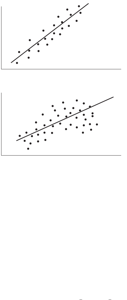
FIGURE 9.4.2 Population conditions relative to

and

that may cause rejection of the null

hypothesis that (

) The relationship between

and

is linear and of sufﬁcient strength

to justify the use of a sample regression equation to predict and estimate

for given values

(

) A linear model provides a good ﬁt to the data, but some curvilinear model would

provide an even better ﬁt.

= 0.

If we measure these deviations for each value of y

and , square each deviation,

and add up the squared deviations, we have

(9.4.2)

total explained unexplained

sum sum sum

of squares of squares of squares

These quantities may be considered measures of dispersion or variability.

Total Sum of Squares The total sum of squares (SST), for example, is a mea-

sure of the dispersion of the observed values of Y about their mean ; that is, this term is

a measure of the total variation in the observed values of Y. The reader will recognize this

term as the numerator of the familiar formula for the sample variance.

Explained Sum of Squares The explained sum of squares measures the

amount of the total variability in the observed values of Y that is accounted for by the

linear relationship between the observed values of X and Y. This quantity is referred to

also as the sum of squares due to linear regression (SSR).

g1y

- y2

= g1y

- y2

+ g1y

- y

426 CHAPTER 9 SIMPLE LINEAR REGRESSION AND CORRELATION

Deep abdominal AT area (cm

), Y

Waist circumference (cm), X

100

120

140

160

180

200

220

240

260

60 65 70 75 80 85 90 95 100 105 110 115 120 125

–

= 101.89

216 + 3.46x

FIGURE 9.4.3 Scatter diagram, sample regression line, and line for Example 9.3.1.y