Daniel W.W. Biostatistics: A Foundation for Analysis in the Health Sciences

Подождите немного. Документ загружается.

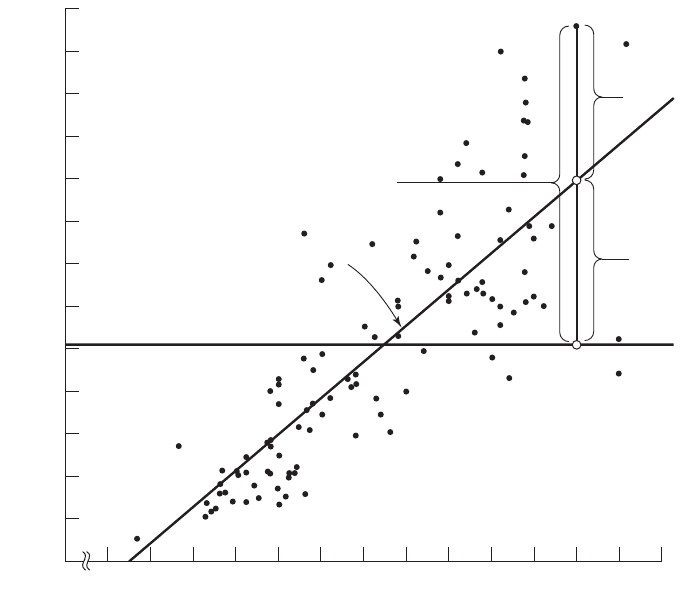
Unexplained Sum of Squares The unexplained sum of squares is a mea-

sure of the dispersion of the observed Y values about the regression line and is sometimes

called the error sum of squares, or the residual sum of squares (SSE). It is this quantity

that is minimized when the least-squares line is obtained.

We may express the relationship among the three sums of squares values as

The numerical values of these sums of squares for our illustrative example appear in

the analysis of variance table in Figure 9.3.2. Thus, we see that

and

Calculating It is intuitively appealing to speculate that if a regression equa-

tion does a good job of describing the relationship between two variables, the explained

or regression sum of squares should constitute a large proportion of the total sum of

354531 = 354531

354531 = 237549 + 116982

SSE = 116982,SSR = 237549,

SST = 354531,

SST = SSR + SSE

9.4 EVALUATING THE REGRESSION EQUATION 427

Deep abdominal AT area (cm

), Y

Waist circumference (cm), X

100

120

140

160

180

200

220

240

260

60 65 70 75 80 85 90 95 100 105 110 115 120 125

–

= 101.89

216 + 3.46x

Total deviation

– y

–

)

Explained

deviation

– y

)

Unexplained

deviation

– y

)

FIGURE 9.4.4 Scatter diagram showing the total, explained, and unexplained

deviations for a selected value of

, Example 9.3.1.

squares. It would be of interest, then, to determine the magnitude of this proportion by

computing the ratio of the explained sum of squares to the total sum of squares. This is

exactly what is done in evaluating a regression equation based on sample data, and the

result is called the sample coefﬁcient of determination, That is,

In our present example we have, using the sums of squares values from Figure 9.3.2,

The sample coefﬁcient of determination measures the closeness of ﬁt of the sample

regression equation to the observed values of Y. When the quantities the vertical

distances of the observed values of Y from the equations, are small, the unexplained sum

of squares is small. This leads to a large explained sum of squares that leads, in turn, to a

large value of This is illustrated in Figure 9.4.5.

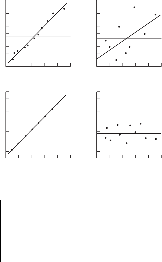
In Figure 9.4.5(a) we see that the observations all lie close to the regression line,

and we would expect to be large. In fact, the computed for these data is .986, indi-

cating that about 99 percent of the total variation in the is explained by the regression.

In Figure 9.4.5(b) we illustrate a case in which the are widely scattered about

the regression line, and there we suspect that is small. The computed for the data

is .403; that is, less than 50 percent of the total variation in the is explained by the

regression.

The largest value that can assume is 1, a result that occurs when all the varia-

tion in the is explained by the regression. When all the observations fall on

the regression line. This situation is shown in Figure 9.4.5(c).

The lower limit of is 0. This result is obtained when the regression line and the

line drawn through coincide. In this situation none of the variation in the is explained

by the regression. Figure 9.4.5(d) illustrates a situation in which is close to zero.

When is large, then, the regression has accounted for a large proportion of the

total variability in the observed values of Y, and we look with favor on the regression

equation. On the other hand, a small which indicates a failure of the regression to

account for a large proportion of the total variation in the observed values of Y, tends

to cast doubt on the usefulness of the regression equation for predicting and estimat-

ing purposes. We do not, however, pass final judgment on the equation until it has

been subjected to an objective statistical test.

Testing with the

Statistic The following example illus-

trates one method for reaching a conclusion regarding the relationship between X and Y.

EXAMPLE 9.4.1

Refer to Example 9.3.1. We wish to know if we can conclude that, in the population

from which our sample was drawn, X and Y are linearly related.

: B

 0

= 1y

- y

237549

354531

= .67

g1y

- y2

g1y

- y2

SSR

SST

428

CHAPTER 9 SIMPLE LINEAR REGRESSION AND CORRELATION

Solution: The steps in the hypothesis testing procedure are as follows:

1. Data. The data were described in the opening statement of Example

9.3.1.

2. Assumptions. We presume that the simple linear regression model and

its underlying assumptions as given in Section 9.2 are applicable.

3. Hypotheses.

a = .05

: b

Z 0

: b

= 0

9.4 EVALUATING THE REGRESSION EQUATION 429

(a)

Close fit, large r

(c)

= 1

(d)

(b)

Poor fit, small r

←

FIGURE 9.4.5 as a measure of closeness-of-ﬁt of the sample regression line to

the sample observations.

4. Test statistic. The test statistic is V.R. as explained in the discussion

that follows.

From the three sums-of-squares terms and their associated degrees

of freedom the analysis of variance table of Table 9.4.1 may be constructed.

In general, the degrees of freedom associated with the sum of

squares due to regression is equal to the number of constants in the regres-

sion equation minus 1. In the simple linear case we have two estimates,

and ; hence the degrees of freedom for regression are

5. Distribution of test statistic. It can be shown that when the hypothesis

of no linear relationship between X and Y is true, and when the assump-

tions underlying regression are met, the ratio obtained by dividing the

regression mean square by the residual mean square is distributed as F

with 1 and degrees of freedom.

6. Decision rule. Reject if the computed value of V.R. is equal to or

greater than the critical value of F.

7. Calculation of test statistic. As shown in Figure 9.3.2, the computed

value of F is 217.28.

8. Statistical decision. Since 217.28 is greater than 3.94, the critical value

of F (obtained by interpolation) for 1 and 107 degrees of freedom, the

null hypothesis is rejected.

9. Conclusion. We conclude that the linear model provides a good ﬁt to

the data.

10. p value. For this test, since we have

■

Estimating the Population Coefﬁcient of Determination The

sample coefﬁcient of determination provides a point estimate of the population coef-

ﬁcient of determination. The population coefﬁcient of determination, has the same

function relative to the population as has to the sample. It shows what proportion of

the total population variation in Y is explained by the regression of Y on X. When the

number of degrees of freedom is small, is positively biased. That is, tends to be

large. An unbiased estimator of is provided by

(9.4.3)r

= 1 -

g1y

- y

>1n - 22

g1y

- y2

>1n - 12

p 6 .005.217.28 7 8.25,

n - 2

2 - 1 = 1.b

430 CHAPTER 9 SIMPLE LINEAR REGRESSION AND CORRELATION

TABLE 9.4.1 ANOVA Table for Simple Linear Regression

Source of

Variation SS

d.f.

MS V.R.

Linear regression

SSR

MSR



SSR/

MSR/MSE

Residual

SSE n

 2

MSE



SSE/

(

 2)

Total

SST n

 1

Observe that the numerator of the fraction in Equation 9.4.3 is the unexplained mean square

and the denominator is the total mean square. These quantities appear in the analysis of

variance table. For our illustrative example we have, using the data from Figure 9.3.2,

This quantity is labeled R-sq(adj) in Figure 9.3.2 and is reported as 66.7 percent. We see

that this value is less than

We see that the difference in and is due to the factor When n is

large, this factor will approach 1 and the difference between and will approach zero.

Testing with the

Statistic When the assumptions stated

in Section 9.2 are met, and are unbiased point estimators of the corresponding

parameters and Since, under these assumptions, the subpopulations of Y values

are normally distributed, we may construct conﬁdence intervals for and test hypotheses

about and . When the assumptions of Section 9.2 hold true, the sampling distri-

butions of and are each normally distributed with means and variances as follows:

(9.4.4)

(9.4.5)

(9.4.6)

and

(9.4.7)

In Equations 9.4.5 and 9.4.7 is the unexplained variance of the subpopulations of Y

values.

With knowledge of the sampling distributions of and we may construct

confidence intervals and test hypotheses relative to and in the usual manner.

Inferences regarding are usually not of interest. On the other hand, as we have seen,

a great deal of interest centers on inferential procedures with respect to . The rea-

son for this is the fact that tells us so much about the form of the relationship

between X and Y. When X and Y are linearly related a positive indicates that, in gen-

eral, Y increases as X increases, and we say that there is a direct linear relationship

between X and Y. A negative indicates that values of Y tend to decrease as values

of X increase, and we say that there is an inverse linear relationship between X and

y>x

g1x

- x2

= b

y>x

ng1x

- x2

= b

: B

 0

1n - 12>1n - 22.r

= 1 -

116982

354531

= .67004

= 1 -

116982>107

354531>108

= .66695

9.4 EVALUATING THE REGRESSION EQUATION 431

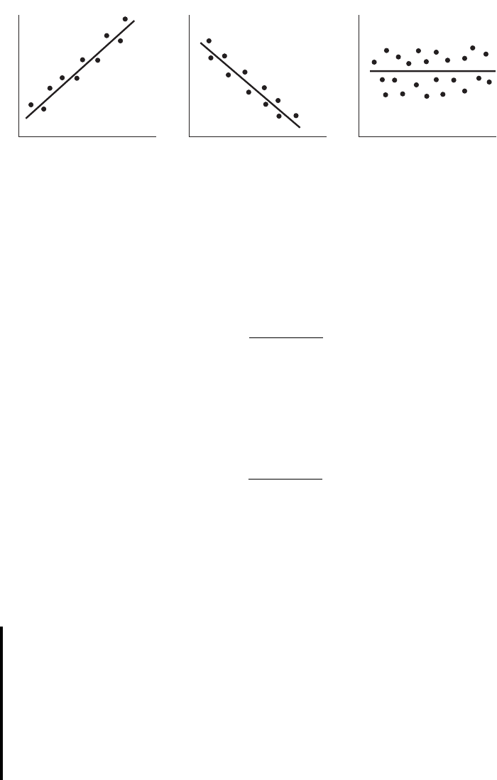
Y. When there is no linear relationship between X and Y, is equal to zero. These

three situations are illustrated in Figure 9.4.6.

The Test Statistic For testing hypotheses about the test statistic when

is known is

(9.4.8)

where is the hypothesized value of . The hypothesized value of does not

have to be zero, but in practice, more often than not, the null hypothesis of interest is

that

As a rule is unknown. When this is the case, the test statistic is

(9.4.9)

where is an estimate of and t is distributed as Student’s t with degrees of

freedom.

If the probability of observing a value as extreme as the value of the test statistic

computed by Equation 9.4.9 when the null hypothesis is true is less than (since we

have a two-sided test), the null hypothesis is rejected.

EXAMPLE 9.4.2

Refer to Example 9.3.1. We wish to know if we can conclude that the slope of the

population regression line describing the relationship between X and Y is zero.

Solution:

1. Data. See Example 9.3.1.

2. Assumptions. We presume that the simple linear regression model and

its underlying assumptions are applicable.

a>2

n - 2s

t =

- 1b

y|x

= 0.

z =

- 1b

y>x

432 CHAPTER 9 SIMPLE LINEAR REGRESSION AND CORRELATION

(a) (b) (c)

FIGURE 9.4.6 Scatter diagrams showing (

) direct linear relationship, (

) inverse

linear relationship, and (

) no linear relationship between

and

3. Hypotheses.

4. Test statistic. The test statistic is given by Equation 9.4.9.

5. Distribution of test statistic. When the assumptions are met and is

true, the test statistic is distributed as Student’s t with degrees of

freedom.

6. Decision rule. Reject if the computed value of t is either greater

than or equal to 1.9826 or less than or equal to

7. Calculation of statistic. The output in Figure 9.3.2 shows that

and

8. Statistical decision. Reject because

9. Conclusion. We conclude that the slope of the true regression line is

not zero.

10. p value. The p value for this test is less than .01, since, when H

is true,

the probability of getting a value of t as large as or larger than 2.6230

(obtained by interpolation) is .005, and the probability of getting a value

of t as small as or smaller than is also .005. Since 14.74 is greater

than 2.6230, the probability of observing a value of t as large as or larger

than 14.74 (when the null hypothesis is true) is less than .005. We double

this value to obtain

Either the F statistic or the t statistic may be used for testing

The value of the variance ratio is equal to the square of

the value of the t statistic i.e., and, therefore, both statistics

lead to the same conclusion. For the current example, we see that

the value obtained by using the F statistic in Exam-

ple 9.4.1.

The practical implication of our results is that we can expect to get

better predictions and estimates of Y if we use the sample regression

equation than we would get if we ignore the relationship between X and

Y. The fact that b is positive leads us to believe that is positive and

that the relationship between X and Y is a direct linear relationship. ■

As has already been pointed out, Equation 9.4.9 may be used to test the null hypothe-

sis that is equal to some value other than 0. The hypothesized value for is

substituted into Equation 9.4.9. All other quantities, as well as the computations, are the

same as in the illustrative example. The degrees of freedom and the method of deter-

mining signiﬁcance are also the same.

114.742

= 217.27,

= F 21

: b

= 0.

21.0052= .01.

-2.6230

14.74 7 1.9826.H

t =

3.4589 - 0

.2347

= 14.74

= .2347,b

= 3.4589,

-1.9826.

n - 2

a = .05

: b

Z 0

: b

= 0

9.4 EVALUATING THE REGRESSION EQUATION 433

A Conﬁdence Interval for Once we determine that it is unlikely, in light

of sample evidence, that is zero, we may be interested in obtaining an interval esti-

mate of The general formula for a conﬁdence interval,

may be used. When obtaining a conﬁdence interval for , the estimator is , the reli-

ability factor is some value of z or t (depending on whether or not is known), and

the standard error of the estimator is

When is unknown, is estimated by

where

In most practical situations our percent conﬁdence interval for is

(9.4.10)

For our illustrative example we construct the following 95 percent confidence

interval for :

We interpret this interval in the usual manner. From the probabilistic point of view we

say that in repeated sampling 95 percent of the intervals constructed in this way will

include The practical interpretation is that we are 95 percent conﬁdent that the sin-

gle interval constructed includes

Using the Conﬁdence Interval to Test

: It is instructive

to note that the conﬁdence interval we constructed does not include zero, so that zero is

not a candidate for the parameter being estimated. We feel, then, that it is unlikely that

This is compatible with the results of our hypothesis test in which we rejected

the null hypothesis that Actually, we can always test at the sig-

niﬁcance level by constructing the percent conﬁdence interval for and

we can reject or fail to reject the hypothesis on the basis of whether or not the interval

includes zero. If the interval contains zero, the null hypothesis is not rejected; and if zero

is not contained in the interval, we reject the null hypothesis.

Interpreting the Results It must be emphasized that failure to reject the null

hypothesis that does not mean that X and Y are not related. Not only is it pos-

sible that a type II error may have been committed but it may be true that X and Y are

related in some nonlinear manner. On the other hand, when we reject the null hypothe-

sis that we cannot conclude that the true relationship between X and Y isb

= 0,

= 0

,10011 - a2

: b

= 0b

= 0.

 0

2.99, 3.92

3.4589 ; 1.98261.23472

; t

11-a>22

b10011 - a2

= MSE

g1x

- x2

g1x

- x2

estimator ; 1reliability factor21standard error of the estimate2

434 CHAPTER 9 SIMPLE LINEAR REGRESSION AND CORRELATION

linear. Again, it may be that although the data ﬁt the linear regression model fairly well

(as evidenced by the fact that the null hypothesis that is rejected), some nonlin-

ear model would provide an even better fit. Consequently, when we reject that

the best we can say is that more useful results (discussed below) may be

obtained by taking into account the regression of Y on X than in ignoring it.

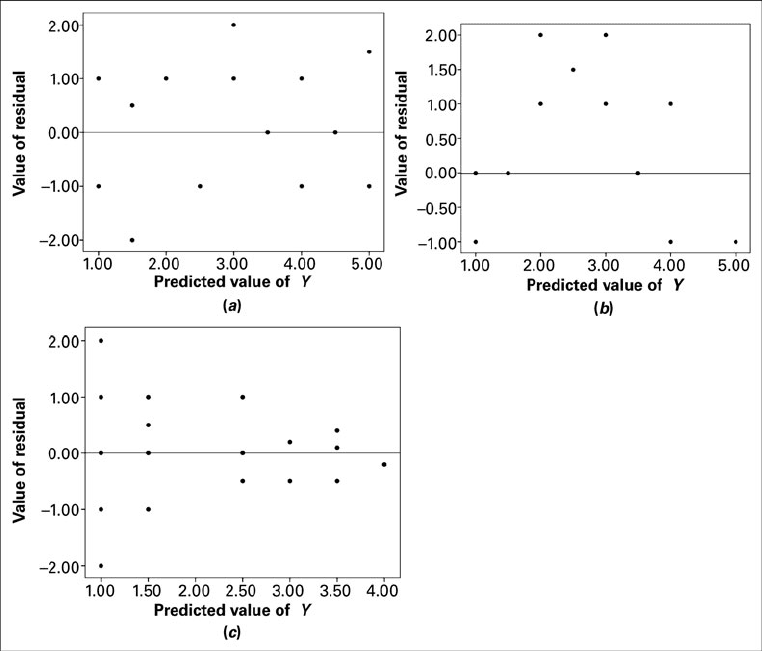
Testing the Regression Assumptions The values of the set of residu-

als, for a data set are often used to test the linearity and equal-variances

assumptions (assumptions 4 and 5 of Section 9.2) underlying the regression model. This

is done by plotting the values of the residuals on the y-axis and the predicted values of

y on the x-axis. If these plots show a relatively random scatter of points above and below

a horizontal line at , these assumptions are assumed to have been met for

a given set of data. A non-random pattern of points can indicate violation of the linear-

ity assumption, and a funnel-shaped pattern of the points can indicate violation of the

equal-variances assumption. Examples of these patterns are shown in Figure 9.4.7. Many

- y

2= 0

- y

= 0,

= 0

9.4 EVALUATING THE REGRESSION EQUATION 435

FIGURE 9.4.7 Residual plots useful for testing the linearity and equal-variances assump-

tions of the regression model. (

) A random pattern of points illustrating non-violation of the

assumptions. (

) A non-random pattern illustrating a likely violation of the linearity assump-

tion. (

) A funneling pattern illustrating a likely violation of the equal-variances assumption.

computer packages will provide residual plots automatically. These plots often use stan-

dardized values i.e., of the residuals and predicted values, but are interpreted

in the same way as are plots of unstandardized values.

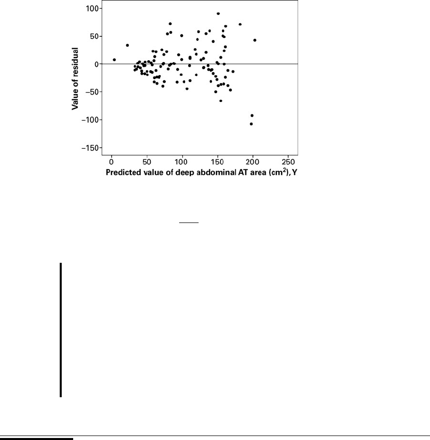
EXAMPLE 9.4.3

Refer to Example 9.3.1. We wish to use residual plots to test the assumptions of linear-

ity and equal variances in the data.

Solution: A residual plot is shown in Figure 9.4.8.

Since there is a relatively equal and random scatter of points above

and below the residual line, the linearity assumption is pre-

sumed to be valid. However, the funneling tendency of the plot suggests

that as the predicted value of deep abdominal AT area increases, so does

the amount of error. This indicates that the assumption of equal variances

may not be valid for these data.

■

EXERCISES

9.4.1 to 9.4.5 Refer to Exercises 9.3.3 to 9.3.7, and for each one do the following:

(a) Compute the coefﬁcient of determination.

(b) Prepare an ANOVA table and use the F statistic to test the null hypothesis that Let

(d) Determine the p value for each hypothesis test.

(e) State your conclusions in terms of the problem.

(f) Construct the 95 percent conﬁdence interval for b

= 0

a = .05.

= 0.

- y

= 0

>1MSE21

436 CHAPTER 9 SIMPLE LINEAR REGRESSION AND CORRELATION

FIGURE 9.4.8 Residual plot of data from Example 9.3.1.