Dan B. Marghitu, Mechanisms and Robots Analysis with MATLAB®
Подождите немного. Документ загружается.


6.3 Lagrange’s Equations for Two-Link Robot Arm 217
Next, the derivative of ∂T /∂ ˙q
i
with respect to time is calculated
d
dt
∂ T
∂ ˙q
1
=
mL
2
6
[8¨q
1
+ 3¨q
2
cos(q
2
−q
1
) −3˙q
2
( ˙q
2
− ˙q
1
) sin(q
2
−q
1
)],
d
dt
∂ T
∂ ˙q
2
=
mL
2
6
[3¨q
1
cos(q
2
−q
1
) −3˙q
1
( ˙q
2
− ˙q
1
) sin(q
2
−q
1
)+2¨q
2
],
and in MATLAB the terms
d
dt
∂ T
∂ ˙q
i
are:
Tt1 = diff(Tdq1, t);
Tt2 = diff(Tdq2, t);
The partial derivative of the kinetic energy with respect to q
i
are
∂ T
∂ q
1
=
mL
2
6
3˙q
1
˙q
2
sin(q
2
−q
1
)=
mL
2
2
˙q
1
˙q
2
sin(q
2
−q
1
);
∂ T
∂ q
2
= −
mL
2
6
3˙q
1
˙q
2
sin(q
2
−q
1
)=−
mL
2
2
˙q
1
˙q
2
sin(q
2
−q
1
),
and with MATLAB:
Tq1 = deriv(T, q1);
Tq2 = deriv(T, q2);
The left-hand side of Lagrange’s equations,
d
dt
∂ T
∂ ˙q
i
−
∂ T
∂ q
i
, with MATLAB are:
LHS1 = Tt1 - Tq1;
LHS2 = Tt2 - Tq2;
Generalized Active Forces
The gravity forces on links 1 and 2 at the mass centers C
1
and C
2
G
1
= −m
1
gj = −mgj and G
2
= −m
2
gj = −mgj.
The torque transmitted from 0 to 1 at A is T
01
= T
01z
k and the torque transmitted
from 1 to 2 at B is T
12
= T
12z
k. The MATLAB commands for the net forces and
moments are:
G1=[0-m1
*
g 0];
G2=[0-m2
*
g 0];
syms T01z T12z
T01 = [0 0 T01z];
T12 = [0 0 T12z];

218 6 Analytical Dynamics of Open Kinematic Chains
There are two generalized forces. The generalized force associated to q
1
is
Q
1
= G
1
·
∂ r
C
1
∂ q
1
+ T
01
·
∂
ω
1
∂ ˙q
1
−T
12
·
∂
ω
1
∂ ˙q
1
+ G
2
·
∂ r
C
2
∂ q
1
+ T
12
·
∂
ω
2
∂ ˙q
1
= −mgj ·(−0.5L sin q
1
ı + 0.5L cos q
1
j)+T
01z
−T
12z
−mgj ·(−L sinq
1
ı + L cosq
1
j)=−1.5mgL cos q
1
+ T
01z
−T
12z
.
The generalized force associated to q
2
is
Q
2
= G
1
·
∂ r
C
1
∂ q
2
+ T
01
·
∂
ω
1
∂ ˙q
2
−T
12
·
∂
ω
1
∂ ˙q
2
+ G
2
·
∂ r
C
2
∂ q
2
+ T
12
·
∂
ω
2
∂ ˙q
2
= −mgj ·(−0.5 L sinq
2
ı + 0.5L cos q
2
j)+T
12z
= −0.5mgL cos q
2
+ T
12z
.
The MATLAB commands for the partial derivatives of the position vectors of the
mass centers,
∂ r
C
1
∂ q
1
,
∂ r
C
2
∂ q
1
,
∂ r
C
1
∂ q
2
,
∂ r
C
2
∂ q
2
are:
rC1
1 = deriv(rC1, q1);
rC2
1 = deriv(rC2, q1);
rC1
2 = deriv(rC1, q2);
rC2
2 = deriv(rC2, q2);
The MATLAB commands for the partial angular velocities,
∂
ω
1
∂ ˙q
1
,
∂
ω
2
∂ ˙q
1
,
∂
ω
1
∂ ˙q
2
,
∂
ω
2
∂ ˙q
2
are:
w1
1 = deriv(omega1, diff(q1,t));
w2
1 = deriv(omega2, diff(q1,t));
w1
2 = deriv(omega1, diff(q2,t));
w2
2 = deriv(omega2, diff(q2,t));
The generalized active forces are calculated with the MATLAB commands:
Q1 = rC1
1
*
G1.’+w1 1
*
T01.’+w1 1
*
(-T12.’)+...
rC2
1
*
G2.’+w2 1
*
T12.’;
Q2 = rC1
2
*
G1.’+w1 2
*
T01.’+w1 2
*
(-T12.’)+...
rC2
2
*
G2.’+w2 2
*
T12.’;

6.3 Lagrange’s Equations for Two-Link Robot Arm 219
The two Lagrange’s equations are
d
dt
∂ T
∂ ˙q
1
−
∂ T
∂ q
1
= Q
1
,
1.333mL
2
¨q
1
+ 0.5mL
2
¨q
2
cos(q
2
−q
1
) −0.5mL
2
˙q
2
2
sin(q
2
−q
1
)
+1.5mgL cos q
1
−T
01z
+ T
12z
= 0;
d
dt
∂ T
∂ ˙q
2
−
∂ T
∂ q
2
= Q
2
,
0.5mL
2
¨q
1
cos(q
2
−q
1
)+0.333mL
2
¨q
2
+ 0.5mL
2
˙q
2
1
sin(q
2
−q
1
)
+0.5mgL cos q
2
−T
12z
= 0, (6.23)
or in MATLAB:
Lagrange1 = LHS1-Q1;
Lagrange2 = LHS2-Q2;
The feedback control laws are
T
01z
= −β
01
˙q
1
−γ
01
(q
1
−q
1 f
)+0.5gL
1
m
1
cos q
1
+ gL
1
m
2
cos q
1
,
T
12z
= −β
12
˙q
2
−γ
12
(q
2
−q
2 f
)+0.5gL
2
m
2
cos q
2
,
with β
01
= 450 Nm s/rad, γ
01
= 300 Nm/rad, β
12
= 200 Nm s/rad, and γ
12
=
300 Nm/rad.
The feedback control torques using MATLAB commands are:
b01 = 450; g01 = 300;
b12 = 200; g12 = 300;
q1f = pi/6;
q2f = pi/3;
T01zc = -b01
*
diff(q1,t)-g01
*
(q1-q1f)+ ...
0.5
*
g
*
L1
*
m1
*
c1+g
*
L1
*
m2
*
c1;
T12zc = -b12
*
diff(q2,t)-g12
*
(q2-q2f)+0.5
*
g
*
L2
*
m2
*
c2;
tor = {T01z, T12z};
torf = {T01zc, T12zc};
The feedback control torques are introduced into Lagrange’s equations:
Lagrang1 = subs(Lagrange1, tor, torf);
Lagrang2 = subs(Lagrange2, tor, torf);
220 6 Analytical Dynamics of Open Kinematic Chains
The numerical data for L
1
, L
2
, m
1
, m
2
, and g are introduced in MATLAB with the
lists:
data = {L1, L2, m1, m2, g };
datn = {1,1,1,1,9.81};
and are substituted into Lagrange’s equations:
Lagran1 = subs(Lagrang1, data, datn);
Lagran2 = subs(Lagrang2, data, datn);
The two second-order Lagrange’s equations have to be rewritten as a first-order sys-
tem and two MATLAB lists are created:
ql={diff(q1,t,2),diff(q2,t,2),...
diff(q1,t),diff(q2,t),q1,q2};
qf={’ddq1’,’ddq2’,’x(2)’,’x(4)’,’x(1)’,’x(3)’};
%ql qf
% ----------------------------
% diff(’q1(t)’,t,2) -> ’ddq1’
% diff(’q2(t)’,t,2) -> ’ddq2’
% diff(’q1(t)’,t) -> ’x(2)’
% diff(’q2(t)’,t) -> ’x(4)’
% ’q1(t)’ -> ’x(1)’
% ’q2(t)’ -> ’x(3)’
In the expression of Lagrange’s equations:
diff(’q1(t)’,t,2) is replaced by ’ddq1’,
diff(’q2(t)’,t,2) is replaced by ’ddq2’,
diff(’q1(t)’,t) is replaced by ’x(2)’,
diff(’q2(t)’,t) is replaced by ’x(4)’,
’q1(t)’ is replaced by ’x(1)’, and
’q2(t)’ is replaced by ’x(3)’
or:
Lagra1 = subs(Lagran1, ql, qf);
Lagra2 = subs(Lagran2, ql, qf);
Lagrange’s equations are solved in terms of ’ddq1’ (¨q
1
) and ’ddq2’ (¨q
2
):
sol = solve(Lagra1,Lagra2,’ddq1, ddq2’);
Lagr1 = sol.ddq1; Lagr2 = sol.ddq2;

6.3 Lagrange’s Equations for Two-Link Robot Arm 221
The system of differential equations is solved numerically by m-file functions. The
function file, RR
Lagr.m is created using the statements:
dx2dt = char(Lagr1);
dx4dt = char(Lagr2);
fid = fopen(’RR
Lagr.m’,’w+’);
fprintf(fid,’function dx = RR
Lagr(t,x)\n’);
fprintf(fid,’dx = zeros(4,1);\n’);
fprintf(fid,’dx(1) = x(2);\n’);
fprintf(fid,’dx(2) = ’);
fprintf(fid,dx2dt);
fprintf(fid,’;\n’);
fprintf(fid,’dx(3) = x(4);\n’);
fprintf(fid,’dx(4) = ’);
fprintf(fid,dx4dt);
fprintf(fid,’;’);
fclose(fid); cd(pwd);
The ode45 solver is used for the system of differential equations
t0 = 0; tf = 15; time = [0 tf];
x0 = [pi/18 0 pi/6 0];
[t,xs] = ode45(@RR
Lagr, time, x0);
x1 = xs(:,1);
x2 = xs(:,2);
x3 = xs(:,3);
x4 = xs(:,4);
subplot(2,1,1),plot(t,x1
*
180/pi,’r’),...
xlabel(’t (s)’),ylabel(’q1 (deg)’),grid,...
subplot(2,1,2),plot(t,x3
*
180/pi,’b’),...
xlabel(’t (s)’),ylabel(’q2 (deg)’),grid
[ts,xs] = ode45(@RR
Lagr,0:1:5,x0);
fprintf(’Results \n\n’)
fprintf(’t(s) q1(rad) dq1(rad/s) q2(rad) dq2(rad/s)\n’)
[ts,xs]
A MATLAB computer program for the direct dynamics is given in the Appendix E.1.
II. Inverse Dynamics
The generalized coordinates are given explicitly for 0 ≤t ≤ T
p
= 15 s
q
r
(t)=q
r
(0)+
q
rf
(T
p
) −q
r
(0)
T
p
t −
T
p
2π
sin
2π t
T
p
, r = 1, 2. (6.24)
222 6 Analytical Dynamics of Open Kinematic Chains
The initial conditions, at t = 0 s, are q
1
(0)=π/18 rad and q
2
(0)=π/6 rad. The
robot arm is brought from an initial state of rest to a final state of rest in such a way
that q
1
and q
2
have the specified values q
1 f
(T
p
)=π/6 rad and q
2 f
(T
p
)=π/3 rad.
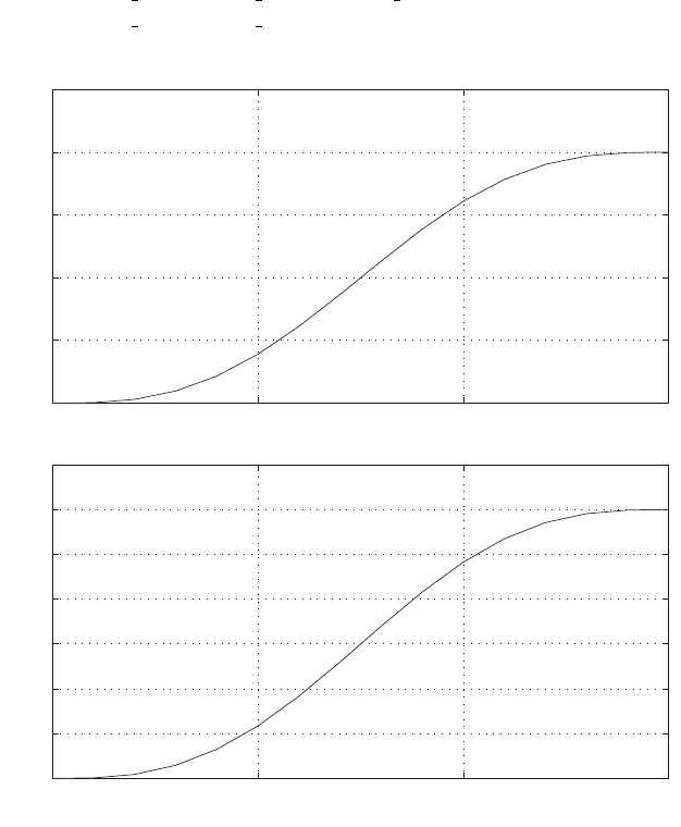
Figure 6.1 shows the plots of q
1
(t) and q
2
(t) rad.
The MATLAB commands for finding Lagrage’s equations are identical with the
commands presented in Direct Dynamics:
........................
syms T01z T12z
T01 = [0 0 T01z];
T12 = [0 0 T12z];
Q1 = rC1
1
*
G1.’+w1 1
*
T01.’+w1 1
*
(-T12.’)+...
rC2
1
*
G2.’+w2 1
*
T12.’;
0 5 10 15
10
15
20
25
30
35
t (s)
q1 (deg)
0 5 10 15
30
35
40
45
50
55
60
65
t (s)
q2 (deg)
Fig. 6.1 Generalized coordinates q
1
(t) and q
2
(t)

6.3 Lagrange’s Equations for Two-Link Robot Arm 223
Q2 = rC1 2
*
G1.’+w1 2
*
T01.’+w1 2
*
(-T12.’)+...
rC2
2
*
G2.’+w2 2
*
T12.’;
Lagrange1 = LHS1-Q1; Lagrange2 = LHS2-Q2;
data = {L1, L2, m1, m2, g};
datn = {1,1,1,1,9.81};
Lagr1 = subs(Lagrange1, data, datn);
Lagr2 = subs(Lagrange2, data, datn);
From Lagrange’s equations of motions the torques T
01z
and T
12z
are calculated:
sol = solve(Lagr1,Lagr2,’T01z, T12z’);
T01zc = sol.T01z;
T12zc = sol.T12z;
The generalized coordinates, q
1
and q
2
, given by Eq. 6.24 and their derivatives,
˙q
1
, ˙q
2
, ¨q
1
, ¨q
2
, are substituted in the expressions of T
01z
and T
12z
:
q1f = pi/6 ; q2f = pi/3;
q1s = pi/18; q2s = pi/6;
Tp=15.;
q1n = q1s+(q1f-q1s)/Tp
*
(t-Tp/(2
*
pi)
*
sin(2
*
pi/Tp
*
t));
q2n = q2s+(q2f-q2s)/Tp
*
(t-Tp/(2
*
pi)
*
sin(2
*
pi/Tp
*
t));
dq1n = diff(q1n,t);
dq2n = diff(q2n,t);
ddq1n = diff(dq1n,t);
ddq2n = diff(dq2n,t);
ql={diff(q1,t,2),diff(q2,t,2),...
diff(q1,t),diff(q2,t),q1,q2};
qn={ddq1n,ddq2n,dq1n,dq2n,q1n,q2n};
%ql qn
% ----------------------------
% diff(’q1(t)’,t,2) -> ddq1n
% diff(’q2(t)’,t,2) -> ddq2n
% diff(’q1(t)’,t) -> dq1n
% diff(’q2(t)’,t) -> dq2n
% ’q1(t)’ -> q1n
% ’q2(t)’ -> q1n
T01zt = subs(T01zc, ql, qn);
T12zt = subs(T12zc, ql, qn);
The MATLAB statement ezplot(f,[min,max]) plots f(t) over the domain:
min<t<max. The plots of T
01z
(t) and T
12z
(t) are obtained with the help of
MATLAB function ezplot:
224 6 Analytical Dynamics of Open Kinematic Chains
subplot(2,1,1), ezplot(T01zt,[0,Tp]),...
title(’’), xlabel(’t (s)’), ylabel(’T01z (N m)’),grid
subplot(2,1,2),ezplot(T12zt,[0,Tp]),...
title(’’), xlabel(’t (s)’), ylabel(’T12z (N m)’),grid
Another way of plotting T
01z
(t) and T
12z
(t) is:
time = 0:1:Tp;
T01t = subs(T01zt,’t’,time);
T12t = subs(T12zt,’t’,time);
subplot(2,1,1),plot(time,T01t),...
xlabel(’t (s)’),ylabel(’T01z (N m)’),grid
subplot(2,1,2),plot(time,T12t),...
xlabel(’t (s)’),ylabel(’T12z (N m)’),grid
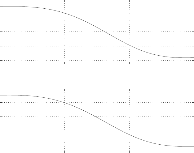
Figure 6.2 shows the control torques and the MATLAB program is given in Ap-
pendix E.2.
0 15
15
16
17
18
19
T01z (N m)
0
5 10
15
2.5
3
3.5
4
t (s)
T12z (N m)
510
t (s)
Fig. 6.2 Control torques
6.4 Rotation Transformation 225
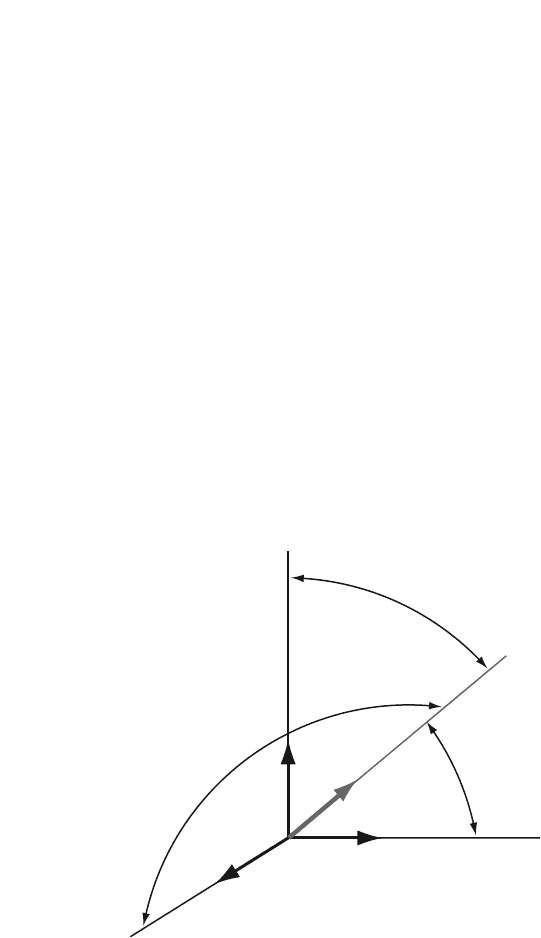
6.4 Rotation Transformation
Two orthogonal reference frames, Oxyz and O
x
y
z
, are considered. The unit vec-
tors of the reference frame Oxyz are ı, j
, k and the unit vectors of the reference frame
O
x
y
z
are ı
, j
, k
. The origins of the reference frames may coincide because only
the orientation of the axes is of interest O = O
.
The angles between the x
-axis and each of the x, y, z axes are the direction an-
gles α, β , and γ (O < α, β,γ < π) as shown in Fig. 6.3. The unit vector ı
can be
expressed in terms of ı, j
, k and the direction angles
ı
=(ı
·ı)ı +(ı
·j)j +(ı
·k)k = cosα ı + cos β j +cosγ k.
The cosines of the direction angles are the direction cosines and cos
2
α + cos
2
β +
cos
2
γ = 1.
With the notations cos α = a
x
x
, cosβ = a
x
y
, and cosγ = a
x
z
the unit vector ı
is
ı
= a
x
x
ı + a
x
y
j + a
x
z
k.
In a similar way, the unit vectors j
and k
are
j
= a
y
x
ı + a
y
y
j + a
y
z
k,
k
= a
z
x
ı + a
z
y
j + a
z
z
k,
where a
r
s
= a
rs
are the cosine of the angle between axis r
and axis s, with r and r
representing x,y,orz. In matrix form
Fig. 6.3 Direction angles
α, β , and γ
O
α
β
γ
k
ı
j
ı
y
z
x
x

226 6 Analytical Dynamics of Open Kinematic Chains
⎡
⎣
ı
j
k
⎤
⎦
= R
⎡
⎣
ı
j
k
⎤
⎦
,
where
R =
⎡
⎣
a
x
x
a
x
y
a
x
z
a
y
x
a
y
y
a
y
z
a
z
x
a
z
y
a
z
z
⎤
⎦
.
The matrix R is the rotation transformation matrix from xyz to x
y
z
. The unit vec-
tors ı,j
,k are an orthogonal set of unit vectors and the unit vectors ı
,j
,k
are an
orthogonal set too. Using these properties it results that
R ·R
T
= I,
where I is the identity matrix. Multiplication of Eq. 6.25 by R
−1
gives
R
−1
= R
T
.
The matrix R is an orthonormal matrix because R
−1
= R
T
.
Let R
be the transformation matrix from ı,j, k to ı
,j
,k
⎡
⎣
ı
j
k
⎤
⎦
= R
⎡
⎣
ı
j
k
⎤
⎦
. (6.25)
The matrix R
is the inverse of the original transformation matrix R, which is iden-
tical to the transpose of R.
R
= R
−1
= R
T
.
Any vector p is independent of the reference frame used to describe its components,
so
p = p
x
ı + p
y
j + p
z
k = p
x
ı
+ p
y
j
+ p
z
k
,
or in matrix form as
[
ı
j
k
]
⎡
⎣
p
x
p
y
p
z
⎤
⎦
=[
ıj
k
]
⎡
⎣
p
x
p
y
p
z
⎤
⎦
.
Using Eq. 6.25 and the fact that the transpose of a product is the product of the