Dan B. Marghitu, Mechanisms and Robots Analysis with MATLAB®

Подождите немного. Документ загружается.

186 5 Direct Dynamics: Newton–Euler Equations of Motion

It is also useful to deﬁne a set of body-ﬁxed coordinate axes. These are axes that

move with the link (body-ﬁxed axes). The n-axis is along the length of the link,

the positive direction running from the origin O toward the mass center C. The unit

vector of the n-axis is n. The t-axis will be perpendicular to the link and be contained

in the plane of motion as shown in Fig. 5.1a.The unit vector of the t-axis is t and

n ×t = k. The velocity of the mass center C in the body-ﬁxed reference frame is

= v

+ ω ×r



ntk

00ω



Lω

t =

t, (5.7)

where r

=(L/2)n. The acceleration of the mass center C in the body-ﬁxed refer-

ence frame is

= a

+ α ×r

−ω

Lα

t −ω

n =

t −

n, (5.8)

= a

+ a

with the components

t and a

= −

Newton–Euler Equation of Motion

The link is rotating about a ﬁxed axis. The mass moment of inertia of the link about

the ﬁxed pivot point O can be evaluated from the mass moment of inertia about the

mass center C using the transfer theorem. Thus

= I

+ m





. (5.9)

The pin is frictionless and is capable of exerting horizontal and vertical forces on

the link at O

= F

01x

ı + F

01y

j, (5.10)

where F

01x

and F

01y

are the components of the pin force on the link in the ﬁxed-axes

system.

The force driving the motion of the link is gravity. The weight of the link is acting

through its mass center and will cause a moment about the pivot point. This moment

will give the link a tendency to rotate about the pivot point. This moment will be

given by the cross product of the vector from the pivot point, O, to the mass center,

C, crossed into the weight force G = −mgj

As the pivot point, O, of the link is ﬁxed, the appropriate moment summation

point will be about that pivot point. The sum of the moments about this point will be

5.1 Compound Pendulum 187

equal to the mass moment of inertia about the pivot point multiplied by the angular

acceleration of the link. The only contributor to the moment is the weight of the

link. Thus we should be able to directly determine the angular acceleration from

the moment equation. The sum of the forces acting on the link should be equal to

the product of the link mass and the acceleration of its mass center. This should be

useful in determining the forces exerted by the pin on the link.

The free-body diagram shows the link at the instant of interest, Fig. 5.1b. The

link is acted upon by its weight acting vertically downward through the mass center

of the link. The link is acted upon by the pin force at its pivot point. The motion

diagram shows the link at the instant of interest, Fig. 5.1c. The motion diagram

shows the relevant acceleration information. The Newton–Euler equations of motion

for the link are

= ΣF = G + F

, (5.11)

α = ΣM

= r

×F

. (5.12)

Since the rigid body has a ﬁxed point at O the equations of motion state that the

moment sum about the ﬁxed point must be equal to to the product of the link mass

moment of inertia about that point and the link angular acceleration. Thus,

α = ΣM

= r

×G. (5.13)

Using Eqs. 5.4, 5.9, and 5.13 the equation of motion is

θk =



ıj

cosθ

sinθ 0

0 −mg 0



, (5.14)

θ = −

cosθ . (5.15)

The equation of motion, Eq. 5.15, is a non-linear, second-order, differential equation

relating the second time derivative of the angle, θ, to the value of that angle and

various problem parameters g and L. The equation is non-linear due to the presence

of the cosθ , where θ(t) is the unknown function of interest.

The force exerted by the pin on the link is obtained from Eq. 5.11

= ma

−G,

and the components of the force are

01x

= m ¨x

= −

(

θ sin θ +

cosθ ),

01y

= m ¨y

+ mg =

(

θ cos θ −

sinθ )+mg. (5.16)

188 5 Direct Dynamics: Newton–Euler Equations of Motion

Using the moving reference frame (body-ﬁxed) the components of the reaction force

on n and t axes are

01n

= ma

−mgsin θ = −

+ mgsin θ,

01t

= ma

−mgcos θ =

+ mgcos θ. (5.17)

If the link is released from rest, then the initial value of the angular velocity is

zero ω(t = 0)=ω(0)=

θ(0)=0 rad/s. If the initial angle is θ (0)=0 radians,

then the cosine of that initial angle is unity and the sine is zero. The initial angular

acceleration can be determined from Eq. 5.15

θ(0)=α(0)=−

cosθ (0)=−

= 16.1 rad/s

. (5.18)

The negative sign indicates that the initial angular acceleration of the link is coun-

terclockwise, as one would expect.

The initial reaction force components can be evaluated from Eq. 5.16

01x

(0)=0lb,

01y

(0)=

θ(0)+mg =

= 3lb.

The equation of motion, Eq. 5.15, is obtained symbolically using the MATLAB



commands:

symsLmgt

omega = [0 0 diff(’theta(t)’,t)];

alpha = diff(omega,t);

c = cos(sym(’theta(t)’));

s = sin(sym(’theta(t)’));

xC = (L/2)

yC = (L/2)

rC = [xC yC 0];

G=[0-m

g 0];

IC=m

Lˆ2/12;

IO=IC+m

(L/2)ˆ2;

MO = cross(rC,G);

eq = -IO

alpha+MO;

eqz = eq(3);

The MATLAB statement diff(X,’t’) or diff(X,sym(’t’)) differentiates

a symbolic expression X with respect to t, and the statement diff(X,’t’,n)

and diff(X,n,’t’) differentiates Xntimes, where n is a positive integer.

An analytical solution to the differential equation is difﬁcult to obtain. Numeri-

cal approaches have the advantage of being simple to apply even for complex me-

5.1 Compound Pendulum 189

chanical systems. The MATLAB function ode45 is used to solve the differential

equation.

The differential equation

θ = −

cosθ is of order 2. The equation has to be

re-written as a ﬁrst-order system. Let x

= θ and x

θ, this gives the ﬁrst-order

system

˙x

= x

˙x

= −

cosx

The MATLAB commands for the right-hand side of the ﬁrst-order system are:

eqI = subs(eqz,{L,m,g},{3,12/32.2,32.2});

eqI1 = subs(eqI,diff(’theta(t)’,t,2),’ddtheta’);

eqI2 = subs(eqI1,diff(’theta(t)’,t),sym(’x(2)’));

eqI3 = subs(eqI2,’theta(t)’,sym(’x(1)’));

dx1 = sym(’x(2)’);

dx2 = solve(eqI3,’ddtheta’);

dx1dt = char(dx1);

dx2dt = char(dx2);

An inline function g is deﬁned for the right-hand side of the ﬁrst-order system.

Note that g must be speciﬁed as a column vector using [...;...] (not a row

vector using [...,...] ). In the deﬁnition of g, x(1) was used for x

and x(2)

was used for x

. The deﬁnition of g should have the form:

g = inline(sprintf(’[%s;%s]’,dx1dt,dx2dt),’t’,’x’);

The statement has to have the form inline(...,’t’,’y’),evenift does not

occur in your formula. The ﬁrst component of g is x(2). The statement sprintf

writes formatted data to string. The time t is going from an initial value t0 to a

ﬁnal value f:

t0=0;

tf = 10;

time = [0 tf];

The initial conditions at t

= 0 are θ(0)=π/4 rad and

θ(0)=0 rad/s or in MAT-

LAB:

x0 = [pi/4; 0]; % define initial conditions

The numerical solution of all the components of the solution for t going from t0

to f is obtained using the command:

190 5 Direct Dynamics: Newton–Euler Equations of Motion

[t,xs] = ode45(g, time, x0);

where x0 is the initial value vector at the starting point t0.

One can obtain a vector t and a matrix xs with the coordinates of these points

using ode45 command.

The vector of x1 values in the ﬁrst column of xs is obtained by using xs(:,1)

and the vector of x2 values in the second column of xs is obtained by using

xs(:,2):

x1 = xs(:,1);

x2 = xs(:,2);

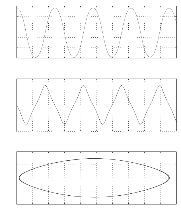
The plot of the solution curves are obtained using the commands:

subplot(3,1,1),plot(t,x1,’r’),...

xlabel(’t’),ylabel(’\theta’),grid,...

subplot(3,1,2),plot(t,x2,’g’),...

xlabel(’t’),ylabel(’\omega’),grid,...

subplot(3,1,3),plot(x1,x2),...

xlabel(’\theta’),ylabel(’\omega’),grid

The plots using MATLAB are shown in Fig. 5.2. In general, the error tends to grow

as one goes further from the initial conditions. To obtain numerical values at speciﬁc

t values one can specify a vector tp of t values and use [ts,xs] = ode45(g,

tp, x0). The ﬁrst element of the vector tp is the initial value and the vector tp

must have at least 3 elements. To obtain the solution with the initial values at t=

0, 0.5, 1.0, 1.5, ... , 10 one can use:

[ts,xs] = ode45(g, 0:0.5:10, x0);

[ts,xs]

and the results are displayed as a table with 3 columns ts, x1 = xs(:,1),

x2 = xs(:,1).

A MATLAB computer program to solve the governing differential equation is

given in Appendix D.1.

The differential equation can be solved numerically by m-ﬁle functions. First

create a function ﬁle, R.m as shown below:

function dx = R(t,x);

dx = zeros(2,1); % a column vector

W=12;L=3;g=32.2; m = W/g;

dx(1) = x(2);

dx(2) = -3

cos(x(1))/(2

L);

5.1 Compound Pendulum 191

012345678910

-4

-3

-2

-1

012345678910

-10

-5

-4 -3.5 -3 -2.5 -2 -1.5 -1 -0.5 0 0.5 1

-10

-5

Fig. 5.2 Plot of solution curves θ and ω =

The ode solver provided by MATLAB (ode45) is used to solve the differential

equation:

tfinal=10;

time=[0 tfinal];

x0=[pi/4 0]; % x(1)(0)=pi/4; x(2)(0)=0

[t,x]=ode45(@R, time, x0);

The MATLAB program is given in Appendix D.2.

192 5 Direct Dynamics: Newton–Euler Equations of Motion

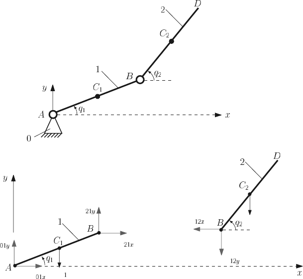
5.2 Double Pendulum

Exercise

A two-link planar chain (double pendulum) is considered, Fig. 5.3a. The links 1 and

2 have the masses m

and m

and the lengths AB = L

and BD = L

. The system

is free to move in a vertical plane. The local acceleration of gravity is g. Numerical

application: m

= m

= 1 kg, L

= 1m,L

= 0.5m,andg = 10 m/s

. Find and solve

the equations of motion.

(a)

(b)

Fig. 5.3 Double pendulum

Solution

The plane of motion is the (x, y) plane with the y-axis vertical, with the positive

sense directed upward. The origin of the reference frame is at A. The mass centers

of the links are designated by C

,0) and C

,0).

The number of degrees of freedom are computed using the relation

5.2 Double Pendulum 193

M = 3n −2c

−c

where n is the number of moving links, c

is the number of one degree of freedom

joints, and c

is the number of two degrees of freedom joints. For the double pendu-

lum n = 2, c

= 2, c

= 0, and the system has two degrees of freedom, M = 2, and

two generalized coordinates. The angles q

(t) and q

(t) are selected as the general-

ized coordinates as shown in Fig. 5.3a.

Kinematics

The position vector of the center of the mass C

of the link 1 is

= x

ı + y

where x

and y

are the coordinates of C

cosq

and y

sinq

The position vector of the center of the mass C

of the link 2 is

= x

ı + y

where x

and y

are the coordinates of C

= L

cosq

and y

= L

sinq

The velocity vector of C

is the derivative with respect to time of the position vector

of C

= ˙x

ı + ˙y

where

˙x

= −

˙q

sinq

and ˙y

˙q

cosq

The velocity vector of C

is the derivative with respect to time of the position vector

of C

= ˙x

ı + ˙y

where

˙x

= −L

˙q

sinq

−

˙q

sinq

and ˙y

= L

˙q

cosq

˙q

cosq

The acceleration vector of C

is the double derivative with respect to time of the

position vector of C

= ¨x

ı + ¨y

where

194 5 Direct Dynamics: Newton–Euler Equations of Motion

¨x

= −

¨q

sinq

−

˙q

cosq

and ¨y

¨q

cosq

−

˙q

sinq

The acceleration vector of C

is the double derivative with respect to time of the

position vector of C

= ¨x

ı + ¨y

where

¨x

= −L

¨q

sinq

−L

˙q

cosq

−

¨q

sinq

−

˙q

cosq

¨y

= L

¨q

cosq

−L

˙q

sinq

¨q

cosq

−

˙q

sinq

The MATLAB commands for the linear accelerations of the mass centers C

and C

are:

L1 = 1; L2 = 0.5; m1 = 1; m2 = 1;g=10;

t = sym(’t’,’real’);

xB=L1

cos(sym(’q1(t)’));

yB=L1

sin(sym(’q1(t)’));

rB = [xB yB 0];

rC1 = rB/2;

vC1 = diff(rC1,t);

aC1 = diff(vC1,t);

xD=xB+L2

cos(sym(’q2(t)’));

yD=yB+L2

sin(sym(’q2(t)’));

rD = [xD yD 0];

rC2 = (rB + rD)/2;

vC2 = diff(rC2,t);

aC2 = diff(vC2,t);

The angular velocity vectors of the links 1 and 2 are

= ˙q

k and ω

= ˙q

The angular acceleration vectors of the links 1 and 2 are

= ¨q

k and α

= ¨q

The MATLAB commands for the angular accelerations of the links 1 and 2 are

omega1 = [0 0 diff(’q1(t)’,t)];

alpha1 = diff(omega1,t);

omega2 = [0 0 diff(’q2(t)’,t)];

alpha2 = diff(omega2,t);

5.2 Double Pendulum 195

Newton–Euler Equations of Motion

The weight forces on the links 1 and 2 are

= −m

gj and G

= −m

gj,

and in MATLAB:

G1=[0-m1

g 0];

G2=[0-m2

g 0];

The mass moment of inertia of the link 1 with respect to the center of mass C

The mass moment of inertia of the link 1 with respect to the ﬁxed point of rotation

A is

= I

+ m





The mass moment of inertia of the link 2 with respect to the center of mass C

The MATLAB commands for the mass moments of inertia are:

IC1=m1

L1ˆ2/12;

IA=IC1+m1

(L1/2)ˆ2;

IC2=m2

L2ˆ2/12;

The equations of motion of the pendulum are inferred using the Newton–Euler

method. There are two rigid bodies in the system and the Newton–Euler equations

are written for each link using the free-body diagrams shown in Fig. 5.3b.

Link 1

The Newton–Euler equations for the link 1 are

= F

+ F

+ G

= r

×F

+ r

×F

where F

is the joint reaction of the ground 0 on the link 1 at point A, and F

the joint reaction of the link 2 on the link 1 at point B

= F

01x

ı + F

01y

and F

= F

21x

ı + F

21y