Dan B. Marghitu, Mechanisms and Robots Analysis with MATLAB®

Подождите немного. Документ загружается.

4.7 R-RTR-RTR Mechanism 175

∑

(4&5)

= r

×(G

+ F

in4

)+r

×F

+ M

in4

×(G

+ F

in5

)+M

in5

+ M

5ext

= 0, (4.85)

where r

= r

−r

, and r

= r

−r

. Equation 4.85 with MATLAB becomes:

eqDR24=cross(rC4-rA,G4+Fin4)+cross(rD-rA,F34)+Min4;

eqDR25=cross(rC5-rA,G5+Fin5)+Me+Min5;

eqDR2=eqDR24+eqDR25;

eqDR2z=eqDR2(3);

The system of two equations is solved using the MATLAB commands:

solF34=solve(eqDR1,eqDR2z);

F34s=[ eval(solF34.F34x), eval(solF34.F34y), 0 ];

The following numerical solution is obtained

= −336.176ı −385.777 j

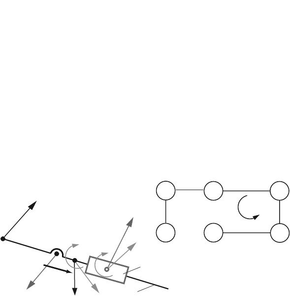
Reaction Force F

The rotation joint C

between the links 0 and 3 is replaced with the unknown reac-

tion force F

(Fig. 4.40)

= F

03x

ı + F

03y

With MATLAB the force F

is written as:

F03=[ sym(’F03x’,’real’), sym(’F03y’,’real’), 0 ];

Following the path I (Fig. 4.40), a force equation is written for the translation joint

. The projection of all forces, that act on the link 3, onto the sliding direction CD

in 2

in 3



(3)

· r



(2&3)

Fig. 4.40 Diagram for calculating the reaction force F

176 4 Dynamic Force Analysis

is zero

∑

(3)

·r

=(F

+ F

+ G

+ F

in3

) ·r

= 0, (4.86)

where r

= r

−r

. Equation 4.86 with the MATLAB command is

eqCR1=dot(F03-F34s+G3+Fin3,rD-rC);

Continuing on the path II (Fig. 4.40), a moment equation is written for the rotation

joint B

∑

(3&2)

= r

×(G

+ F

in3

)+r

×F

+ r

×F

+ M

in2

+ M

in3

= 0, (4.87)

where r

= r

−r

, r

= r

−r

, and r

= r

−r

. With MATLAB Eq. 4.87

gives:

eqCR2=cross(rC3-rB,G3+Fin3)+cross(rC-rB,F03)+...

cross(rD-rB,-F34s)+Min2+Min3;

eqCR2z=eqCR2(3);

To solve the system of two equations the MATLAB commands are used:

solF03=solve(eqCR1,eqCR2z);

F03s=[ eval(solF03.F03x), eval(solF03.F03y), 0 ];

The following numerical solution is obtained

= −431.027ı −878.152 j N.

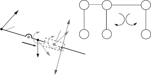
Reaction Force F

The translation joint B

between the links 2 and 3 is replaced with the unknown

reaction force F

(Fig. 4.41)

= −F

= F

23x

ı + F

23y

The position of the application point Q of the force F

is unknown

= x

ı + y

where x

and y

are the plane coordinates of the point Q. The force F

and its point

of application Q are written in MATLAB as:

F23=[ sym(’F23x’,’real’), sym(’F23y’,’real’), 0 ];

F32=-F23;

rQ=[ sym(’xQ’,’real’), sym(’yQ’,’real’), 0 ];

Following the path I (Fig. 4.41), a moment equation is written for the rotation joint

4.7 R-RTR-RTR Mechanism 177

in 2

in 3



(2)



(3)

Fig. 4.41 Diagram for calculating the reaction force F

∑

(3)

= r

×F

+ r

×(G

+ F

in3

)+r

×F

+ M

in3

= 0, (4.88)

where r

= r

−r

, r

= r

−r

, and r

= r

−r

. Using MATLAB, Eq. 4.88

is written as:

eqBT1=cross(rQ-rC,F23)+cross(rC3-rC,G3+Fin3)+...

cross(rD-rC,-F34s)+Min3;

eqBT1z=eqBT1(3);

Following the path II (Fig. 4.41), a moment equation is written for the rotation joint

∑

(2)

= r

×F

+ M

in2

= 0, (4.89)

where r

= r

−r

. Equation 4.89 with MATLAB becomes:

eqBT2=cross(rQ-rB,F32)+Min2;

eqBT2z=eqBT2(3);

The direction of the unknown joint force F

is perpendicular to the sliding direction

BC. The following relation is written

·r

= 0,

or with MATLAB, it is:

eqF23BC=dot(F23,rC-rB);

The application point Q of the force F

is located in the direction BC, that is

−r

) ×(r

−r

)=0. (4.90)

178 4 Dynamic Force Analysis

Equation 4.90 with MATLAB gives:

eqQ=cross(rB-rC,rQ-rC);

eqQz=eqQ(3);

The system of four equations is solved using the MATLAB command:

solF23=solve(eqBT1z,eqBT2z,F23BC,eqQz);

F23s=[ eval(solF23.F23x), eval(solF23.F23y), 0 ];

rQs=[ eval(solF23.xQ), eval(solF23.yQ), 0 ];

The following numerical solutions are obtained

= 94.8233ı + 492.717 j N and r

= 0.129904ı + 0.075 j m.

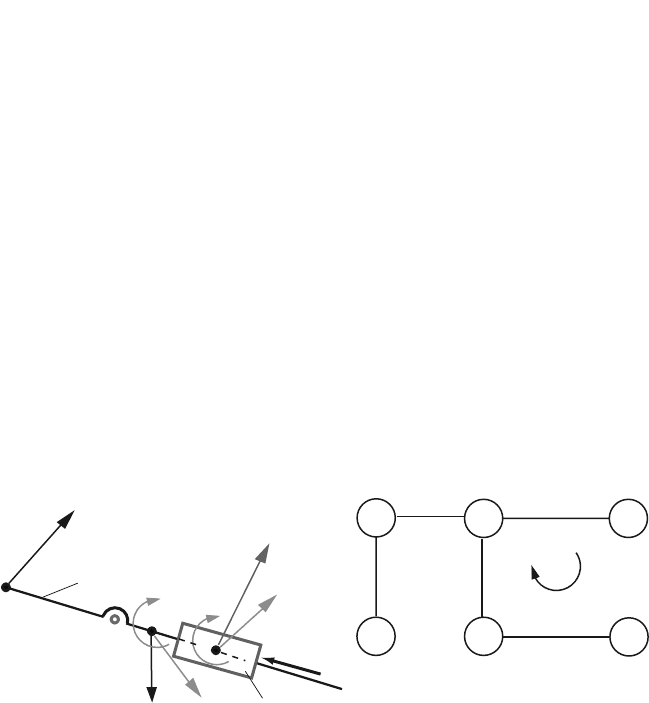
Reaction Force F

The rotation joint B

between the links 1 and 2 is replaced with the unknown reac-

tion force F

(Fig. 4.42)

= −F

= F

12x

ı + F

12y

With MATLAB it is written as:

F12=[ sym(’F12x’,’real’), sym(’F12y’,’real’), 0 ];

F21=-F12;

Following the path I (Fig. 4.42), a force equation is written for the translation joint

. The projection of all forces, that act on the link 2, onto the sliding direction BC

is zero

∑

(2)

·r

=(F

+ G

+ F

in2

) ·r

= 0. (4.91)

in 2

in 3



(2)

· r



(2&3)

Fig. 4.42 Diagram for calculating the reaction force F

4.7 R-RTR-RTR Mechanism 179

Using MATLAB it is written as:

eqBR1=dot(F12+G2+Fin2,rC-rB);

Continuing on the path I, a moment equation is written for the rotation joint C

∑

(2&3)

= r

×F

+ r

×(G

+ F

in2

)+M

in2

×(G

+ F

in3

)+r

×F

+ M

in3

= 0, (4.92)

where r

= r

−r

, r

= r

−r

, r

= r

−r

, and r

= r

−r

. Using

the MATLAB, commands Eq. 4.92 gives:

eqBR2=cross(rB-rC,F12)+cross(rC2-rC,G2+Fin2)+Min2...

+cross(rC3-rC,G3+Fin3)+cross(rD-rC,-F34s)+Min3;

eqBR2z=eqBR2(3);

The system of two equations is solved using the MATLAB commands:

solF12=solve(eqBR1,eqBR2z);

F12s=[ eval(solF12.F12x), eval(solF12.F12y), 0 ];

and the following numerical solution is obtained

= 94.7949ı + 492.779 j

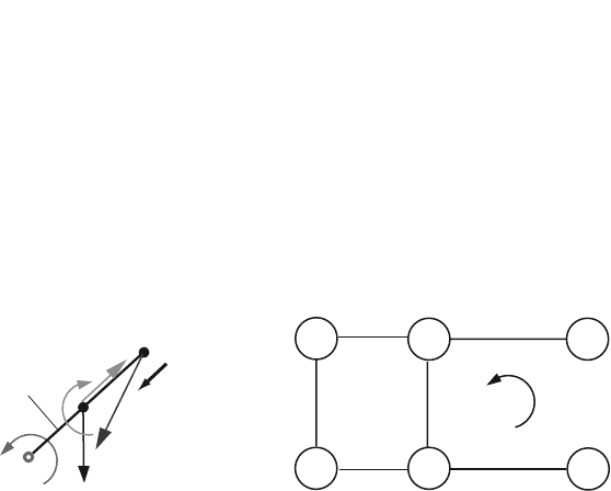
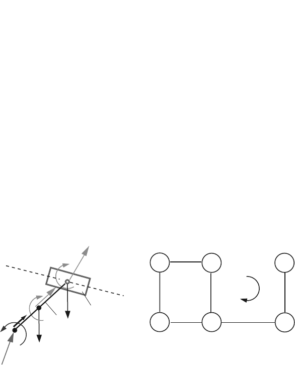
Motor Moment M

mot

The motor moment needed for the dynamic equilibrium of the mechanism is M

mot

k (Fig. 4.43). Following the path I (Fig. 4.43), a moment equation is written

for the rotation joint A

∑

(1)

= r

×F

+ r

×(G

+ F

in1

)+M

in1

+ M

mot

= 0. (4.93)



(1)

mot

in 1

mot

Fig. 4.43 Diagram for calculating the motor moment M

mot

180 4 Dynamic Force Analysis

Equation 4.93 is solved using the MATLAB command:

M1m=-(cross(rB,-F12s)+cross(rC1,G1+Fin1)+Min1);

The numerical solution is

mot

= 56.9119 k Nm.

Reaction Force F

The rotation joint A

between the links 0 and 1 is replaced with the unknown reac-

tion force F

(Fig. 4.44)

= −F

= F

01x

ı + F

01y

With MATLAB it is written as:

F01=[ sym(’F01x’,’real’), sym(’F01y’,’real’), 0 ];

Following the path I (Fig. 4.44), a moment equation is written for the rotation joint

∑

(1)

= r

×F

+ r

×(G

+ F

in1

)+M

in1

+ M

mot

= 0, (4.94)

where r

= −r

, and r

= r

−r

. Equation 4.94 using the MATLAB com-

mands gives:

eqAAR1=cross(-rB,F01)+cross(rC1-rB,G1+Fin1)+Min1+M1m;

eqAAR1z=eqAAR1(3);

Continuing on the path I (Fig. 4.44), a force equation is written for the translation

joint B



(1)

mot

in 1

in 2



F · r

(1&2)

Fig. 4.44 Diagram for calculating the reaction force F

4.7 R-RTR-RTR Mechanism 181

The projection of all forces, that act on the links 1 and 2, onto the sliding direction

BC is zero

∑

(1&2)

·r

=(F

+ G

+ F

in1

+ G

+ F

in2

) ·r

= 0, (4.95)

or with MATLAB it is:

eqAAR2=dot(F01+G1+Fin1+G2+Fin2,rC-rB);

The system of two equations is solved using the MATLAB commands:

solF01=solve(eqAAR1z, eqAAR2);

F01s=[ eval(solF01.F01x), eval(solF01.F01y), 0 ];

The following numerical solution is obtained

= 94.7736ı + 492.884 j N.

The MATLAB program for the dynamic force analysis is presented in Appendix C.7.

Chapter 5

Direct Dynamics: Newton–Euler Equations of

Motion

The Newton–Euler equations of motion for a rigid body in plane motion are

∑

F and I

Czz

α =

∑

or using the Cartesian components

m ¨x

∑

, m ¨y

∑

, and I

Czz

θ =

∑

The forces and moments are known and the differential equations are solved for the

motion of the rigid body (direct dynamics).

5.1 Compound Pendulum

Exercise

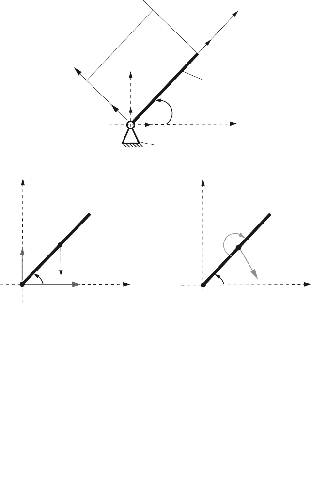
Figure 5.1a depicts a compound pendulum of mass m and length L. The pendulum

is connnected to the ground by a pin joint and is free to swing in a vertical plane.

The link is moving and makes an instant angle θ(t) with the horizontal. The local

acceleration of gravity is g. Numerical application: L = 3 ft, g = 32.2 ft/s

, G =

mg = 12 lb. Find and solve the Newton–Euler equations of motion.

Solution

The system of interest is the link during the interval of its motion. The link in rota-

tional motion is constrained to move in a vertical plane. First, a reference frame will

be introduced. The plane of motion will be designated the (x, y) plane. The y-axis is

vertical, with the positive sense directed vertically upward. The x-axis is horizontal

and is contained in the plane of motion. The z-axis is also horizontal and is perpen-

dicular to the plane of motion. These axes deﬁne an inertial reference frame. The

unit vectors for the inertial reference frame are ı, j

, and k. The angle between the x

and the link axis is denoted by θ . The link is moving and hence the angle is chang-

ing with time at the instant of interest. In the static equilibrium position of the link,

183

184 5 Direct Dynamics: Newton–Euler Equations of Motion

01x

01y

(a)

(

)

(c)

m a

Fig. 5.1 Compound pendulum

the angle, θ , is equal to −π/2. The system has one degree of freedom. The angle,

θ, is an appropriate generalized coordinate describing this degree of freedom. The

system has a single moving body. The only motion permitted that body is rotation

about a ﬁxed horizontal axis (z-axis). The body is connected to the ground with the

rotating pin joint (R) at O. The mass center of the link is at the point C. As the link

is uniform, its mass center is coincident with its geometric center.

Kinematics

The mass center, C, is at a distance L/2 from the pivot point O and the position

vector is

= r

= x

ı + y

j, (5.1)

where x

and y

are the coordinates of C

5.1 Compound Pendulum 185

cosθ and y

sinθ . (5.2)

The link is constrained to move in a vertical plane, with its pinned location, O,

serving as a pivot point. The motion of the link is planar, consisting of pure rotation

about the pivot point. The directions of the angular velocity and angular acceleration

vectors will be perpendicular to this plane, in the z-direction.The angular velocity

of the link can be expressed as

ω = ωk =

dθ

k =

θk, (5.3)

ω is the rate of rotation of the link. The positive sense is clockwise (consistent with

the x and y directions deﬁned above). This problem involves only a single moving

rigid body and the angular velocity vector refers to that body. For this reason, no

explicit indication of the body, 1, is included in the speciﬁcation of the angular

velocity vector

ω = ω

. The angular acceleration of the link can be expressed as

α =

ω = αk =

k =

θk, (5.4)

α is the angular acceleration of the link. The positive sense is clockwise.

The velocity of the mass center can be related to the velocity of the pivot point

using the relationship between the velocities of two points attached to the same rigid

body

= v

+ ω ×r



ıj

00ω



= ω(−y

ı + x

Lω

(−sin θı + cos θj

). (5.5)

The velocity of the pivot point, O, is zero. The acceleration of the mass center can be

related to the acceleration of the pivot point (a

= 0) using the relationship between

the accelerations of two points attached to the same rigid body

= a

+ α ×r

+ ω ×(ω ×r

)=a

+ α ×r

−ω



ıj

00α



−ω

ı + y

j)=α(−y

ı + x

j) −ω

ı + y

= −(αy

+ ω

)ı +(αx

−ω

= −

(α sin θ + ω

cosθ )ı +

(α cos θ −ω

sinθ )j

= −

(

θ sin θ +

cosθ )ı +

(

θ cos θ −

sinθ )j. (5.6)