Dake L.P. Fundamentals of reservoir engineering

Подождите немного. Документ загружается.

SOME BASIC CONCEPTS IN RESERVOIR ENGINEERING 30

depletion line

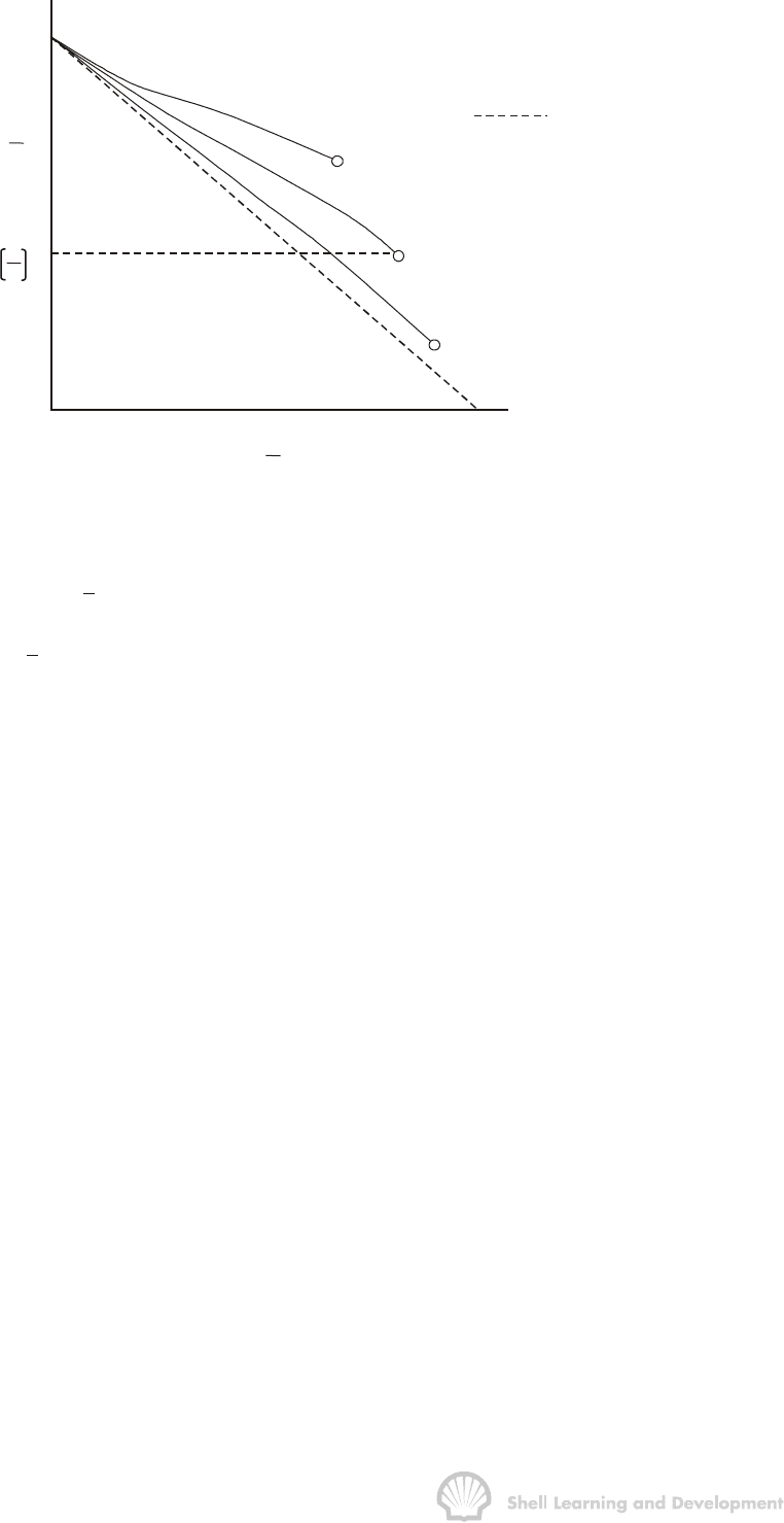
Fig. 1.11 Graphical representation of the material balance equation for a water drive

gas reservoir, for various aquifer strengths; equ. (1.41)

WcWp=∆

where c =the total aquifer compressibility (c

+ c

)

W =the total volume of water, and depends primarily on the geometry of

the aquifer

and

p∆=the pressure drop at the original reservoir-aquifer boundary.

This model assumes that, because the aquifer is relatively small, a pressure drop in the

reservoir is instantaneously transmitted throughout the entire reservoir-aquifer system.

The material balance in such a case would be as shown by plot A in fig. 1.11, which is

not significantly different from the depletion line.

To provide the pressure response shown by lines B and C, the aquifer volume must be

considerably larger than that of the reservoir and it is then inadmissible to assume

instantaneous transmission of pressure throughout the system. There will now be a

time lag between a pressure perturbation in the reservoir and the full aquifer response.

To build an aquifer model, including this time dependence, is quite complex and the

subject will be deferred until Chapter 9 where the use of such a model for both history

matching and prediction will be described in detail.

One of the unfortunate aspects in the delay in aquifer response is that, initially, all the

material balance plots in fig. 1.11 appear to be linear and, if there is insufficient

production and pressure history to show the deviation from linearity, one may be

tempted to extrapolate the early trends, assuming a depletion type reservoir, which

would result in the determination of too large a value of the GIIP. In such a case, a

large difference between this and the volumetric estimate of the GIIP can be diagnostic

in deciding whether there is an aquifer or not. It also follows that attempting to build a

SOME BASIC CONCEPTS IN RESERVOIR ENGINEERING 31

mathematical model to describe the reservoir performance based on insufficient history

data can produce erroneous results when used to predict future reservoir performance.

If production-pressure history is available it is possible to make an estimate of the GIIP,

in a water drive reservoir, using the following method as described by Bruns et.al

. The

depletion material balance, equ. (1.34), is first solved to determine the apparent gas in

place as

1E/E

−

(1.42)

If there is an active water drive, the value of G

calculated using this equation, for

known values of E and G

, will not be unique. Successive, calculated values of G

will

increase as the deviation of p/Z above the depletion material balance line increases,

due to the pressure maintenance provided by the aquifer. The correct value of the gas

in place, however, can be obtained from equ. (1.40) as

GWE

1E/E

−

—

(1.43)

where W

is the cumulative water influx calculated, using some form of mathematic

aquifer model, at the time at which both E and G

have been measured.

- too small

- correct model

- too large

E/ (1−E / E

)

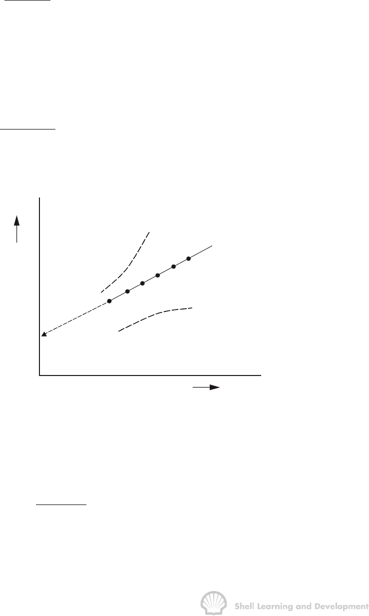
Fig. 1.12 Determination of the GIIP in a water drive gas reservoir. The curved, dashed

lines result from the choice of an incorrect, time dependent aquifer model;

(refer Chapter 9)

Subtracting equ. (1.43) from equ. (1.42) gives

1E/E

−

(1.44)

If the calculated values of G

, equ. (1.42), are plotted as a function of W

E/(1−E/E

) the

result should be a straight line, provided the correct aquifer model has been selected,

SOME BASIC CONCEPTS IN RESERVOIR ENGINEERING 32

as shown in fig. 1.12, and the proper value of G can be determined by linear

extrapolation to the ordinate. Selecting the correct aquifer model (aquifer fitting) is a

trial and error business which continues until a straight line is obtained.

One other interesting feature shown in fig. 1.11 is that the maximum possible gas

recovery, shown by the circled points, depends on the degree of pressure maintenance

afforded by the aquifer, being smaller for the more responsive aquifers. The reason for

this has already been mentioned in sec. 1.2; that in the immiscible displacement of one

fluid by another not all of the displaced fluid can be removed from each pore space.

Thus as the water advances through the reservoir a residual gas saturation is trapped

behind the front. This gas saturation, S

, is rather high being of the order of 30−50% of

the pore volume

7,17

, and is largely independent of the pressure at which the gas is

trapped. This being the case, then applying the equation of state, equ. (1.15), to the

gas trapped per cu.ft of pore volume behind the flood front, gives

SnRT

and, since S

is independent of pressure, then for isothermal depletion

∝

which indicates that a greater quantity of gas is trapped at high pressure than at low.

The ultimate gas recovery depends both on the nature of the aquifer and the

abandonment pressure. For the value of (p/Z)

shown in fig. 1.11, the aquifer giving

the pressure response corresponding to line B is the most favourable. While choice of

the abandonment pressure is under the control of the engineer, the choice of the

aquifer, unfortunately, is not. It is, therefore, extremely important to accurately measure

both pressures and gas production to enable a reliable aquifer model to be built which,

in turn, can be used for performance predictions.

One of the more adventurous aspects of gas reservoir engineering is that gas sales

contracts, specifying the market rate and pipeline pressure, are usually agreed

between operator and purchaser very early in the life of the field, when the amount of

history data is minimal. The operator is then forced to make important decisions on

how long he will be able to meet the market demand, based on the rather scant data.

Sensitivity studies are usually conducted at this stage, using the simple material

balance equations presented in this chapter, and varying the principal parameters, i.e.

− the GIIP

− the aquifer model, based on the possible geometrical configurations of the aquifer

− abandonment pressure; whether to apply surface compression or not

− the number of producing wells and their mechanical design.

SOME BASIC CONCEPTS IN RESERVOIR ENGINEERING 33

(the latter point has not been discussed so far, since it requires the development of well

inflow equations, which will be described in Chapter 8). The results of such a study can

give initial guidance on the best way to develop the gas reserve.

EXERCISE 1.2 GAS MATERIAL BALANCE

The following data are available for a newly discovered gas reservoir:

GWC = 9700 ft

Centroid depth = 9537 ft

Net bulk volume (V) = 1.776 × 10

cu.ft

=0.19

=0 20

=0.85

Although a gas sample was collected during a brief production test the reservoir

pressure was not recorded because of tool failure. It is known, however, that the water

pressure regime in the locality is

= 0.441D + 31 psia

and that the temperature gradient is 1.258°F/100 ft, with ambient surface temperature

80° F.

1) Calculate the volume of the GIIP.

2) It is intended to enter a gas sales contract in which the following points have

been stipulated by the purchaser.

a) during the first two years, a production rate build-up from zero

−100 MMscf/d (million) must be achieved while developing the field

b) the plateau rate must be continued for 15 years at a sales point delivery

pressure which corresponds to a minimum reservoir pressure of 1200 psia.

Can this latter requirement be fulfilled? (Assume that the aquifer is small so

that the depletion material balance equation can be used).

3) Once the market requirement can no longer be satisfied the field rate will decline

exponentially by 20% per annum until it is reduced to 20 MMscf/d. (This gas will

either be used as fuel in the company's operations or compressed to supply part

of any current market requirement).

What will be the total recovery factor for the reservoir and what is the length of the

entire project life?

EXERCISE 1.2 SOLUTION

a) In order to determine the GIIP it is first necessary to calculate the initial gas

pressure at the centroid depth of the reservoir. That is, the depth at which there is

SOME BASIC CONCEPTS IN RESERVOIR ENGINEERING 34

as much gas above as there is beneath, the pressures for use in the material

balance equation will always be evaluated at this depth.

To do this the water pressure at the gas−water contact must first be calculated as

= 0.441 × 9700 + 31 = 4309 psia =

GWC

and the temperature as

9700

T (1.258 ) 80 460 662 R

100

=×++=

for this 0.85 gravity gas the isothermal Z−factor plot at 200°F (660°R), fig. 1.8,

can be used to determine the Z−factor at the GWC, with negligible error. Thus

GWC

= 0.888

and E

GWC

= 35.37

p 35.37 4309

259.3

ZT 0.888 662

The pressure gradient in the gas, at the GWC, can now be calculated, as

described in exercise 1.1, as

dp 0.0763 0.85 259.3

0.117 psi / ft

dD 144 144

××

== =

The gas pressure at the centroid is therefore

GWC

pp D

æö

=− ×∆

ç÷

èø

(1.45)

p = 4309 − 0.117 × (9700 − 9537) = 4290 psia

and the absolute temperature at the centroid is

9537

T (1.258 ) 80 460 660 R

100

=×++=

One could improve on this estimate by re−evaluating the gas gradient at the

centroid, for p = 4290 psia and T = 660°R, and averaging this value with the

original value at the GWC to obtain a more reliable gas gradient to use in

'equ. (1.45). Gas gradients are generally so small, however, that this correction is

seldom necessary. The reader can verify that, in the present case, the correction

would only alter the centroid pressure by less than half of one psi.

For the centroid pressure and temperature of 4290 psia and 660°R, the GIIP can

be estimated as

GIIP = G = V

(1−S

) E

(1.26)

SOME BASIC CONCEPTS IN RESERVOIR ENGINEERING 35

1.776x10 0.19 0.8 35.37 4290

699.70 10 scf

0.887 660

××× ×

==×

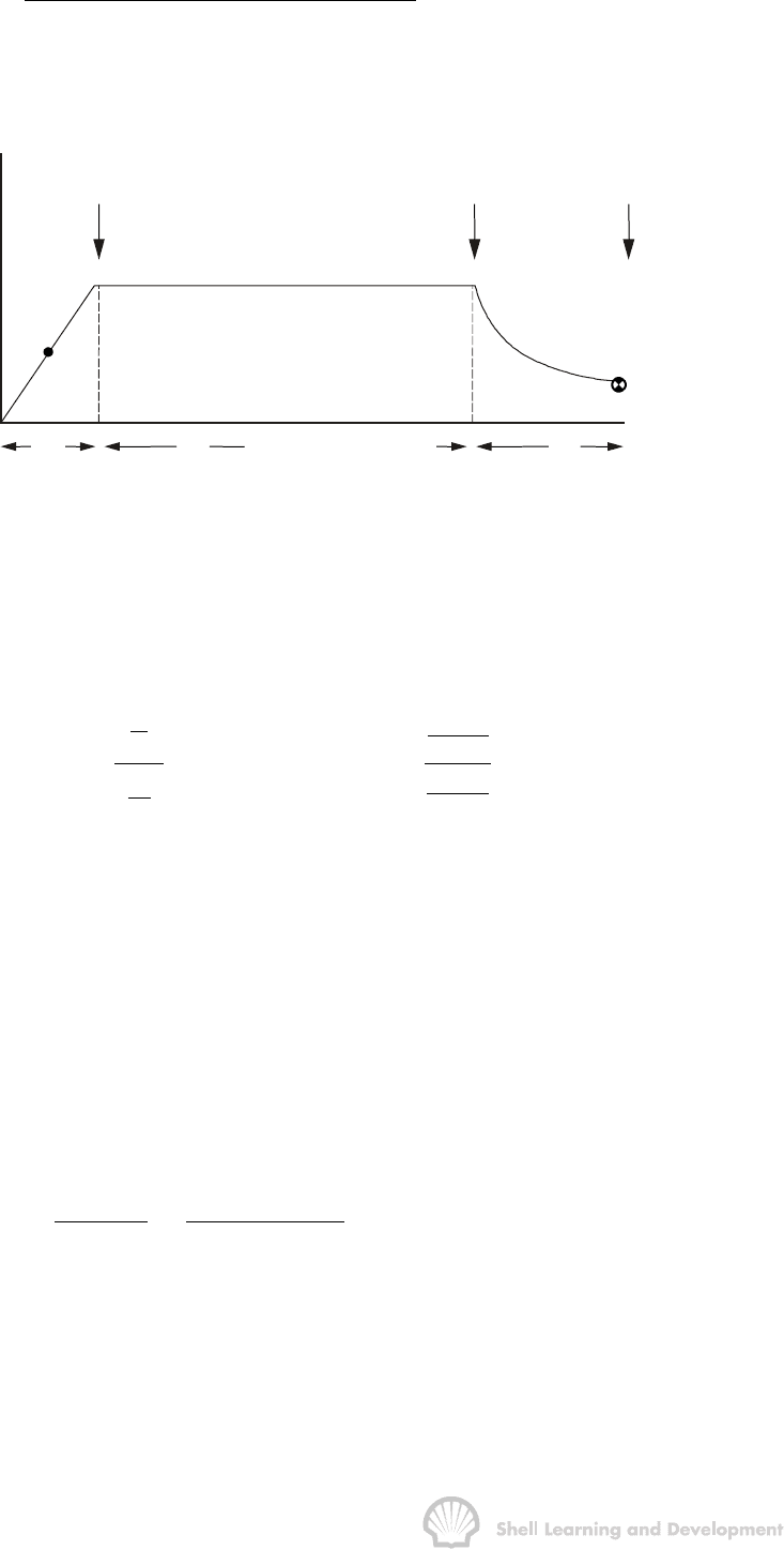
2) The overall production schedule can be divided into three parts, the build-up,

plateau production and decline periods, as shown in fig. 1.13.

= 100 (MMscf/d)

50 (MMscf /d)

Rate

(MMscf /d)

20 (MMscf /d)

Fig. 1.13 Gas field development rate−

−−

−time schedule (Exercise 1.2)

It is first required, to determine

G , that is, the cumulative production when the

reservoir pressure has fallen to 1200 psia and the plateau rate can no longer be

maintained. When p = 1200 psia, Z = 0.832 (fig. 1.8) and using the depletion

material balance, equ. (1.35),

1200

0.832

GG(1 )699.7010(1 )

4290

0.887

G 491.04 10 scf

æö

ç÷

èø

=− = × =

æö

ç÷

èø

=×

Since the cumulative production during the two years build-up period is

G = Q

avg

× 2 × 365 = 50 × 10

× 2 × 365 = 36.5 × 10

scf

the gas production at the plateau rate of 100 MMscf/d is

G −

G = (491.04 – 36.50) × 10

= 454.54 × 10

scf

and the time for which this rate can be maintained is

454.54 10

t12.45yrs

100 10 365

−

== =

××

Therefore the time for which the plateau rate can be sustained will fall short of the

requirement by some 2.5 years.

3) During the exponential decline period the rate at any time after the start of the

decline can be calculated as

SOME BASIC CONCEPTS IN RESERVOIR ENGINEERING 36

QQe=

−bt

where Q

is the rate at t = 0, i.e. 100 MMscf/d, and b is the exponential decline

factor of 0.2 p.a. Therefore, the time required for the rate to fall to 20 MMscf/d will

11100

tln ln 8.05yrs

bQ0.220

== =

If g

is the cumulative gas production at time t, measured from the start of the

decline, then

g Qdt Q e dt

−

òò

i.e.

g(1e)

−

=−

and when t = 8.05 yrs.

(8.05)

100 10 365

0.2 8.05

g (1 e ) 146.02 10 scf

0.2

××

−×

=−=×

Therefore, the total cumulative recovery at abandonment will be

32(8.05)

ppp

G G g (491.04 146.02) 10 637.06 10 scf=+ = + ×= ×

and the recovery factor

637.06 10

RF 0.91 or 91% GIIP

699.70 10

== =

which will be recovered after a total period of

+ t

= 2 + 12.45 + 8.05 = 22.5 years.

This simple exercise covers the spectrum of reservoir engineering activity,

namely, estimating the hydrocarbons in place, calculating a recovery factor and

attaching a time scale to the recovery. The latter is imposed by the overall market

rate required of the field, i.e.

cumulative production

time

field rate

Later in the book, in Chapters 4, 6 and 8, the method of calculating individual well

rates is described, which means that the time scale can be fixed by the more

usual type of expression.

SOME BASIC CONCEPTS IN RESERVOIR ENGINEERING 37

()

12 2

wpw

m p 3.161 10 FQ

βγ

−

∆=× =

1.8 HYDROCARBON PHASE BEHAVIOUR

This subject has been covered extensively in specialist books

8,13,18

and is described

here in a somewhat perfunctory manner simply to provide a qualitative understanding

of the difference between various hydrocarbon systems as they exist in the reservoir.

Consider, first of all, the simple experiment in which a cylinder containing one of the

lighter members of the paraffin series, C

−ethane, is subjected to a continuously

increasing pressure at constant temperature. At some unique pressure (the vapour

pressure) during this experiment the C

, which was totally in the gas phase at low

pressures will condense into a liquid. If this experiment were repeated at a series of

different temperatures the resulting phase diagram, which is the pressure temperature

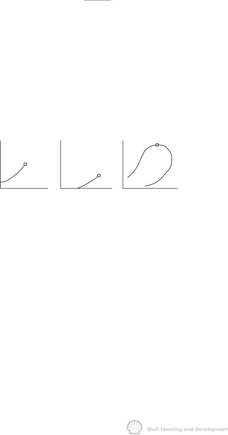
relationship, could be drawn as shown in fig. 1.14(a).

100% - C

50% - C

PP P

LIQUID

GAS

LIQUID

GAS

GAS GAS

( a )

( b )

( c )

Fig. 1.14 Phase diagrams for (a) pure ethane; (b) pure heptane and (c) for a 50−

−−

−50

mixture of the two

The line defining the pressures at which the transition from gas to liquid occurs, at

different temperatures, is known as the vapour pressure line. It terminates at the critical

point (CP) at which it is no longer possible to distinguish whether the fluid is liquid or

gas, the intensive properties of both phases being identical. Above the vapour pressure

line the fluid is entirely liquid while below it is in the gaseous state.

If the above experiment were repeated for a heavier member of the paraffin series, say,

− heptane, the results would be as shown in fig. 1.14(b). One clear difference

between (a) and (b) is that at lower temperatures and pressures there is a greater

tendency for the heavier hydrocarbon, C

, to be in the liquid state.

For a two component system, the phase diagram for a 50% C

and 50% C

mixture would be as shown in fig. 1.14 (c). In this case, while there are regions where

the fluid mixture is either entirely gas or liquid, there is now also a clearly defined

region in which the gas and liquid states can coexist; the, so-called, two phase region.

The shape of the envelope defining the two phase region is dependent on the

composition of the mixture, being more vertically inclined if the C

is the predominant

component and more horizontal if it is the C

SOME BASIC CONCEPTS IN RESERVOIR ENGINEERING 38

Naturally occurring hydrocarbons are more complex than the system shown in fig. 1.14

in that they contain a great many members of the paraffin series and usually some non-

hydrocarbon impurities. Nevertheless, a phase diagram can similarly be defined for

complex mixtures and such a diagram for a typical natural gas is shown in fig. 1.15(a).

The lines defining the two phase region are described as the bubble point line,

separating the liquid from the two phase region, and the dew point line, separating the

gas from the two phase region. That is, on crossing the bubble point line from

90%

70%

50%

30%

10%

LIQUID

( a )

LIQUID

( b )

GAS GAS

Fig. 1.15 Schematic, multi-component, hydrocarbon phase diagrams; (a) for a natural

gas; (b) for oil

liquid to the two phase region, the first bubbles of gas will appear while, crossing the

dew point line from the gas, the first drops of liquid (dew) will appear. The lines within

the two phase region represent constant liquid saturations.

For a gas field, as described in secs. 1.5 − 1.8, the reservoir temperature must be such

that it exceeds the so-called cricondentherm (CT), which is the maximum temperature

at which the two phases can coexist for the particular hydrocarbon mixture. If the initial

reservoir pressure and temperature are such that they coincide with point A in

fig. 1.15(a), then for isothermal reservoir depletion, which is generally assumed, the

pressure will decline from A towards point B and the dew point line will never be

crossed. This means that only dry gas will exist in the reservoir at any pressure. On

producing the gas to the surface, however, both pressure and temperature will

decrease and the final state will be at some point X within the two phase envelope, the

position of the point being dependent on the conditions of surface separation.

The material balance equations presented in this chapter, equs. (1.35) and (1.41),

assumed that a volume of gas in the reservoir was produced as gas at the surface. If,

due to surface separation, small amounts of liquid hydrocarbon are produced, the

cumulative liquid volume must be converted into an equivalent gas volume and added

to the cumulative gas production to give the correct value of G

for use in the material

balance equation.

SOME BASIC CONCEPTS IN RESERVOIR ENGINEERING 39

Thus if n pound moles of liquid have been produced, of molecular weight M, then the

total mass of liquid is

nM =

× (liquid volume)

where γ

is the oil gravity (water = 1), and

is the density of water (62.43 Ib/cu.ft).

Since liquid hydrocarbon volumes are generally measured in stock tank barrels

(1 bbl = 5.615 cu.ft), then the number of pound moles of liquid hydrocarbon produced in

stb is

n350.5

Expressing this number of moles of hydrocarbon as an equivalent gas volume at

standard conditions, gives

nRT

10.732 520

V 350.5

p M 14.7

or V 1.33 10

== ×

=×

The correction in adding the equivalent gas volume to the cumulative gas production is

generally rather small, of the order of one percent or less, and is sometimes neglected.

If the initial reservoir pressure and temperature are such that the gas is at point C,

fig. 1.15(a), then during isothermal depletion liquid will start to condense in the

reservoir when the pressure has fallen below the dew point at D.

The maximum liquid saturation deposited in the reservoir, when the pressure is

between points D and E in the two phase region, is generally rather small and

frequently is below the critical saturation which must be exceeded before the liquid

becomes mobile. This phenomenon is analogous to the residual saturations, discussed

previously, at which flow ceases. Therefore, the liquid hydrocarbons deposited in the

reservoir, which are referred to as retrograde liquid condensate, are not recovered and,

since the heavier components tend to condense first, this represents a loss of the most

valuable part of the hydrocarbon mixture. It may be imagined that continued pressure

depletion below the dew point at E would lead to re-vapourisation of the liquid

condensate. This does not occur, however, because once the pressure falls below

point D the overall molecular weight of the hydrocarbons remaining in the reservoir

increases, since some of the heavier paraffins are left behind in the reservoir as

retrograde condensate. Therefore, the composite phase envelope for the reservoir

fluids tends to move downwards and to the right thus inhibiting re-vapourisation.

It is sometimes economically viable to produce a gas condensate field by the process

of dry gas re-cycling. That is, from the start of production at point C, fig. 1.15(a),

separating the liquid condensate from the dry gas at the surface and re-injecting the

latter into the reservoir in such a way that the dry gas displaces the wet gas towards

the producing wells. Since only a relatively small amount of fluid is removed from the

reservoir during this process, the pressure drop is small and, for a successful project,