Coburn J.W., Herdlick J.D. College Algebra: Graphs and Models

Подождите немного. Документ загружается.

370 CHAPTER 3 Quadratic Functions and Operations on Functions 3–90

College Algebra G&M—

1. ____

2. ____

3. ____ ,

4. ____ ,

5. ____ ,

6. ____ ,

7. ____

8. ____ y ⫽ 31x ⫺ 22

⫺ 5

y ⫽⫺x

⫹ 4

b 6 0m 7 0

b 7 0m 6 0

1x2T for x 僆 12, q2

1x2c for x 僆 1⫺q, 22

1x2c for x 僆 12, q2

1x2T for x 僆 1⫺q, 22

y ⫽⫺

x ⫹ 1

1x ⫹ 12

⫹ 1y ⫺ 22

⫽ 4

9. ____ center

10. ____ vertex (2, 5), y-intercept (0, 1)

11. ____

12. ____

13. ____ axis of symmetry ,

opens downward

14. ____

15. ____ for ,

for

16. ____ , f

112⫽⫺3f 1⫺22⫽ 0

x 僆 3⫺2, 24f

1x2ⱖ 0

x 僆 1⫺q,⫺22 ´ 12, q2f

1x26 0

4x ⫺ 3y ⫽ 3

x ⫽ 2

1x ⫺ 12

⫹ 1y ⫹ 22

⫽ 9

y ⫽

1x ⫺ 12

⫺ 3

radius ⫽ 311, ⫺22,

SECTION 3.1 Complex Numbers

KEY CONCEPTS

•

The italicized i represents the number whose square is This means and

•

Larger powers of i can be simpliﬁed using

•

For and we say the expression has been written in terms of i.

•

The standard form of a complex number is where a is the real number part and bi is the imaginary part.

•

To add or subtract complex numbers, combine the like terms.

•

For any complex number its complex conjugate is

•

The product of a complex number and its conjugate is a real number.

a ⫺ bi.a ⫹ bi,

a ⫹ bi,

k 7 0, 1⫺k

⫽ i1k

⫽ 1.

i ⫽ 1⫺1

⫽⫺1⫺1.

SUMMARY AND CONCEPT REVIEW

Making Connections: Graphically, Symbolically, Numerically, and Verbally

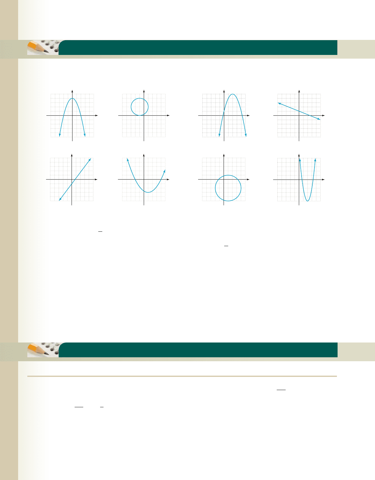
Eight graphs (a) through (h) are given. Match the characteristics shown in 1 through 16 to one of the eight graphs.

5⫺5

⫺5

5⫺5

⫺5

5⫺5

⫺5

5⫺5

⫺5

(a) (b) (c) (d)

5⫺5

⫺5

5⫺5

⫺5

5⫺5

⫺5

5⫺5

⫺5

(e) (f) (g) (h)

MAKING CONNECTIONS

cob19545_ch03_353-370.qxd 11/25/10 3:53 PM Page 370

3–91 Summary and Concept Review 371

College Algebra G&M—College Algebra G&M—

•

The commutative, associative, and distributive properties also apply to complex numbers and are used to perform

basic operations.

•

To multiply complex numbers, use the F-O-I-L method and simplify.

•

To ﬁnd a quotient of complex numbers, multiply the numerator and denominator by the conjugate of the denominator.

EXERCISES

Simplify each expression and write the result in standard form.

1. 2. 3.

4. 5.

Perform the operation indicated and write the result in standard form.

6. 7. 8.

9. 10.

Use substitution to show the given complex number and its conjugate are solutions to the equation shown.

11. 12.

SECTION 3.2 Solving Quadratic Equations and Inequalities

KEY CONCEPTS

•

The standard form of a quadratic equation is where a, b, and c are real numbers and In

words, we say the equation is written in decreasing order of degree and set equal to zero.

•

A quadratic function is one that can be written as , where a, b, and c are real numbers and .

•

The following four statements are equivalent: (1) is a solution of , (2) r is a zero of f(x), (3) (r, 0) is

an x-intercept of , and (4) is a factor of f(x).

•

The square root property of equality states that if where then or

•

Quadratic equations can also be solved by completing the square, or using the quadratic formula.

•

If the discriminant the equation has one real (repeated) root. If the equation has

two real roots; and if the equation has two nonreal roots.

•

Quadratic inequalities can be solved using the zeroes of the function and either an understanding of quadratic

graphs or mid-interval test values.

EXERCISES

13. Solve by factoring.

a. b. c. d.

14. Solve using the square root property of equality.

a. b. c. d.

15. Solve by completing the square. Give real number solutions in exact and approximate form.

a. b. c. d.

16. Solve using the quadratic formula. Give solutions in both exact and approximate form.

a. b. c.

17. Solve by locating the x-intercepts and noting the end-behavior of the graph.

a. b. c.

18. Solve using the interval test method.

a. b. c. x

⫹ 4x ⫹ 4 ⱕ 0x

7 20 ⫺ xx

⫹ 3x ⱕ 4

⫺ 2x ⫹ 2 7 0⫺x

⫹ 1 ⱖ 0x

⫺ x ⫺ 6 7 0

⫺ 6x ⫹ 5 ⫽ 04x

⫹ 7 ⫽ 12xx

⫺ 4x ⫽⫺9

⫺ 7x ⫽⫺2⫺4x ⫹ 2x

⫽ 3x

⫹ 6x ⫽ 16x

⫹ 2x ⫽ 15

⫺2x

⫹ 4 ⫽⫺463x

⫹ 15 ⫽ 021x ⫺ 22

⫹ 1 ⫽ 11x

⫺ 9 ⫽ 0

⫺ 3x

⫽ 4x ⫺ 123x

⫺ 15 ⫽ 4x2x

⫺ 50 ⫽ 0x

⫺ 3x ⫺ 10 ⫽ 0

⫺ 4ac 6 0,

⫺ 4ac 7 0,b

⫺ 4ac ⫽ 0,

X ⫽⫺1k

.X ⫽ 1kk ⱖ 0,X

⫽ k,

1x ⫺ r2y ⫽ f

1x2

1x2⫽ 0x ⫽ r

a ⫽ 0f

1x2⫽ ax

⫹ bx ⫹ c

a ⫽ 0.ax

⫹ bx ⫹ c ⫽ 0,

⫺ 4x ⫹ 9 ⫽ 0; x ⫽ 2 ⫹ i25x

⫺ 9 ⫽⫺34; x ⫽ 5i

4i1⫺3 ⫹ 5i212 ⫹ 3i212 ⫺ 3i2

1⫺3 ⫹ 5i2⫺ 12 ⫺ 2i2

1 ⫺ 2i

15 ⫹ 2i2

131⫺6

⫺10 ⫹ 1⫺50

61⫺481⫺72

cob19545_ch03_371-380.qxd 8/10/10 8:09 PM Page 371

Solve the following quadratic applications. For 19 and 20, recall the height of a projectile is modeled by

19. A projectile is ﬁred upward from ground level with an initial velocity of 96 ft/sec. (a) To the nearest tenth of a

second, how long until the object ﬁrst reaches a height of 100 ft? (b) How long until the object is again at 100 ft?

20. A person throws a rock upward from the top of an 80-ft cliff with an initial velocity of 64 ft/sec. (a) To the nearest

tenth of a second, how long until the object is 120 ft high? (b) How long until the object is again at 120 ft?

SECTION 3.3 Quadratic Functions and Applications

KEY CONCEPTS

•

The graph of a quadratic function is a parabola. Parabolas have three distinctive features: (1) like end-behavior on

the left and right, (2) an axis of symmetry, (3) a highest or lowest point called the vertex.

•

By completing the square, can be written as the transformation and

graphed using transformations of

•

For a quadratic function in the standard form

•

End-behavior: graph opens upward if opens downward if

•

Zeroes/x-intercepts (if they exist): substitute 0 for y and solve for x

•

y-intercept: substitute 0 for

•

Vertex: (h, k), where

•

Maximum value: If the parabola opens downward, is the maximum value of f.

•

Minimum value: If the parabola opens upward, is the minimum value of f.

•

Line of symmetry: is the line of symmetry. If is on the graph, then is also on the graph.

EXERCISES

Graph p(x) and f(x) by completing the square and using transformations of the parent function. Graph g(x) and h(x)

using the vertex formula and y-intercept. Find the x-intercepts (if they exist) for all functions.

21. 22. 23. 24.

25. Height of a superball: A teenager tries to see how high she can bounce her superball by throwing it downward on

her driveway. The height of the ball (in feet) at time t (in seconds) is given by (a) How high

is the ball at (b) How high is the ball after 1.5 sec? (c) How long until the ball is 135 ft high? (d) What is

the maximum height attained by the ball? At what time t did this occur?

26. Theater Revenue: The manager of a large, 14-screen movie theater ﬁnds that if he charges $2.50 per person for

the matinee, the average daily attendance is 4000 people. With every increase of 25 cents the attendance drops an

average of 200 people. (a) What admission price will bring in a revenue of $11,250? (b) How many people will

purchase tickets at this price?

SECTION 3.4 Quadratic Models; More on Rates of Change

KEY CONCEPTS

•

Regardless of the form of regression chosen, obtaining a regression equation uses these ﬁve steps: (1) clear out old

data, (2) enter new data, (3) set an appropriate window and display the data, (4) calculate the regression equation,

and (5) display the data and equation, and once satisﬁed the model is appropriate, apply the result.

•

The choice of a nonlinear regression model often depends on many factors, particularly the context of the data,

any patterns formed by the scatterplot, some foreknowledge on how the data might be related, and/or a careful

assessment of the correlation coefﬁcient.

•

Applications of quadratic regression are generally applied when a set of data indicates a gradual decrease to some

minimum value, with a matching increase afterward, or a gradual increase to some maximum, with a matching

decrease afterward.

t ⫽ 0?

h1t2⫽⫺16t

⫹ 96t.

h1x2⫽ 4x

⫺ 12x ⫹ 3g1x2⫽⫺x

⫹ 4x ⫺ 5f 1x2⫽ x

⫹ 8x ⫹ 15p1x2⫽ x

⫺ 6x

1h ⫺ c, y21h ⫹ c, y2x ⫽ h

y ⫽ k

h ⫽

⫺b

, k ⫽ f a

⫺b

x S 10, c2

a 6 0a 7 0,

y ⫽ ax

⫹ bx ⫹ c,

y ⫽ x

1x2⫽ a1x ⫹ h2

⫾ k,f 1x2⫽ ax

⫹ bx ⫹ c

h ⫽⫺16t

⫹ v

t ⫹ k.

372 CHAPTER 3 Quadratic Functions and Operations on Functions 3–92

College Algebra G&M—

cob19545_ch03_371-380.qxd 11/25/10 3:55 PM Page 372

•

For nonlinear functions, the average rate of change gives an average value for how changes in the independent

variable cause a change in the dependent variable within a speciﬁed interval.

•

The average rate of change is given by the slope of a secant line through two points (x

, y

) and (x

, y

) on the

graph, and is computed as: .

EXERCISES

27. While the Internet has been with us for over 20 years, its use continues to grow at a

rapid pace. The data in the table gives the amount of money (in billions of dollars)

consumers spent online for retail items in selected years (amounts for 2010 through

2012 are projections). Use the data and a graphing calculator to (a) draw a scatterplot

and decide on an appropriate form of regression, then (b) ﬁnd the regression equation

and use it to estimate the amount spent by consumers in 2003, (c) the projected

amount that will be spent in 2014 if this rate of growth continues, and (d) the year

that $591 billion is the projected amount of retail spending over the Internet.

28. The drag force on a compact car driving along the highway on a windless day,

depends on a constant and the velocity of the car, where k is determined using the

density of the air, the cross-sectional area of the car, and the drag coefﬁcient of the

vehicle. The data shown in the table gives the magnitude of the drag force F

, at given

velocity v. Use the data and a graphing calculator to (a) draw a scatterplot and decide

on an appropriate form of regression, then (b) ﬁnd a regression equation and use it to

estimate the magnitude of the drag force for this car at 60 mph. Finally, (c) estimate the

speed of the car if the drag force has a magnitude of 2329 units.

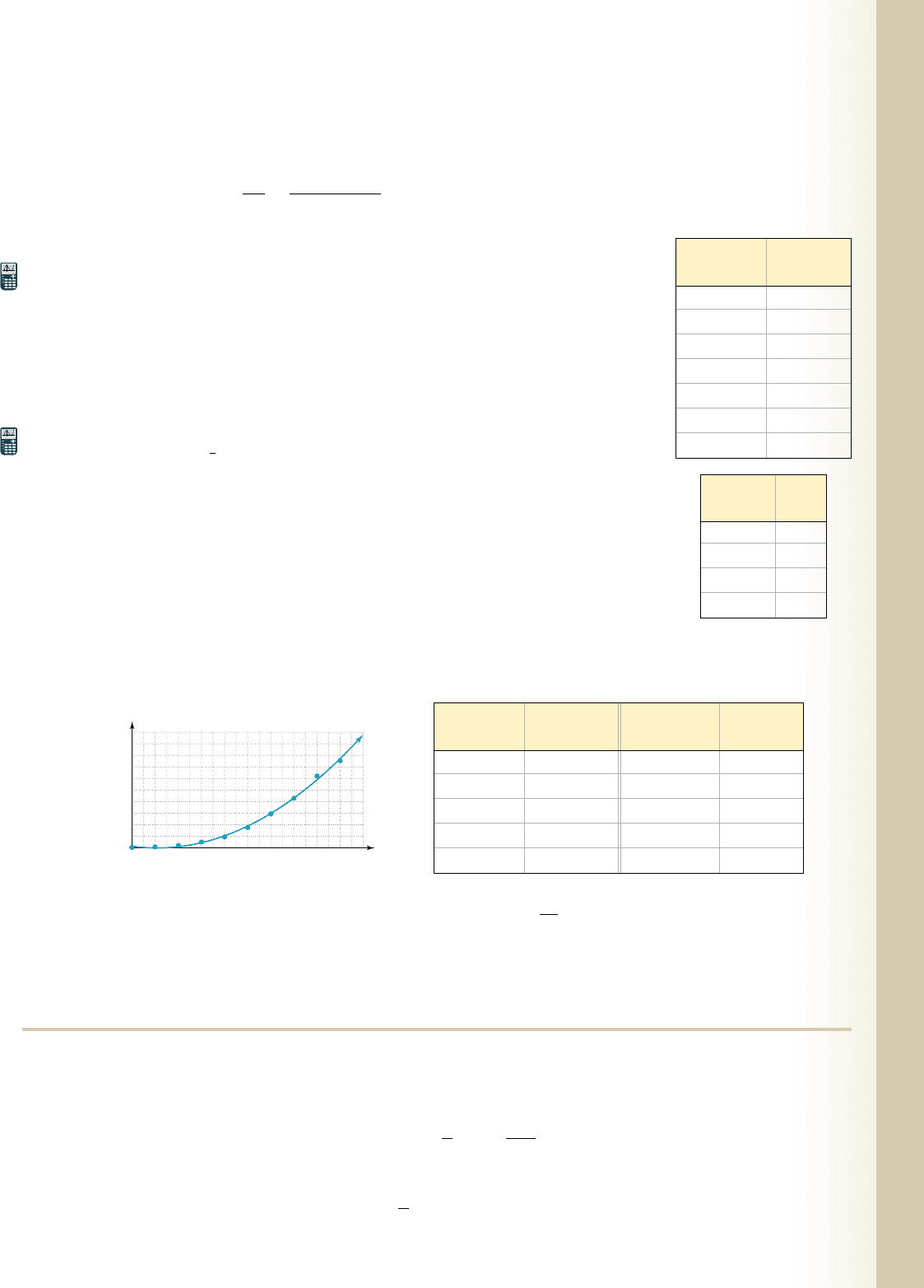
29. The graph and accompanying table show the number N of active Starbucks outlets for

selected years t from 1990 to 2008. Use the graph and table to (a) ﬁnd the average rate of

change for the years 1994 to 1996 (the interval [4, 6]). (b) Verify that the rate of growth between the years 2000

and 2002 (the interval [10, 12]) was about 4 times greater than from 1994 to 1996. (c) Show that the average rate

of change for the years 2002 to 2004 was very close to the rate of change for the years 2006 to 2008.

¢y

¢x

⫽

2⫺ f 1x

⫺ x

, x

⫽ x

3–93 Summary and Concept Review 373

College Algebra G&M—College Algebra G&M—

020

Year (t)

18161412108642

120

200

160

Outlets (N)

Year t Outlets N Year t Outlets N

(1990 → 0) (100s) (1990 → 0) (100s)

0 0.84 10 35.01

2 1.65 12 58.86

4 4.25 14 85.69

6 10.15 16 124.40

8 18.86 18 150.79

30. According to Torricelli’s law for tank draining, the volume (in ft

) of a full bathtub t sec after

the plug is pulled can be modeled by the function . (a) What is the volume of the bathtub

at ? (b) What is the volume of the bathtub at ? (c) What is the average rate of change from

to ? (d) What is the average rate of change from to ? (e) When is the bathtub empty?

SECTION 3.5 The Algebra of Functions

KEY CONCEPTS

•

The notation used to represent the basic operations on two functions is

••

•

The result of these operations is a new function h(x). The domain of h is the intersection of domains for f and g,

excluding values that make for .h1x2⫽ a

b1x2g1x2⫽ 0

b1x2⫽

1x2

g1x2

; g1x2⫽ 01f

g21x2⫽ f 1x2

g1x2

1f ⫺ g21x2⫽ f

1x2⫺ g1x21f ⫹ g21x2⫽ f 1x2⫹ g1x2

t ⫽ 21t ⫽ 20t ⫽ 1

t ⫽ 0t ⫽ 1 sect ⫽ 0 sec

V1t2⫽ 1⫺0.2t ⫹ 120

5 ft ⫻ 2 ft ⫻ 2 ft

Velocity

(mph)

10 32

30 306

50 860

70 1694

Year Amount

(2000 S 0) (billions)

131

584

6 108

7 128

10 267

11 301

12 335

cob19545_ch03_371-380.qxd 11/25/10 3:55 PM Page 373

374 CHAPTER 3 Quadratic Functions and Operations on Functions 3–94

College Algebra G&M—

EXERCISES

For and ﬁnd the following:

31. 32. 33. the domain of

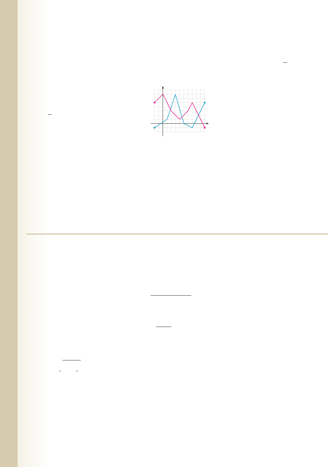
34. Use the graph given to ﬁnd the value of each expression:

35. As the availability of free, public Wi-Fi has increased, so has the number of devices that can utilize this protocol.

A new company has just released a Wi-Fi phone that provides free phone service anywhere it has access to a

wireless network. The total cost for manufacturing these phones can be modeled by the function

, where n is the number of phones made and C(n) is in dollars. If each phone is

sold at a price of $84.95, the revenue is modeled by .

a. Find the function that represents the total proﬁt made from sales of the phones.

b. How much proﬁt is earned if 400 phones are sold?

c. How much proﬁt is earned if 5000 phones (the production limit) are sold?

R1n2⫽ 84.95n

C1n2⫽⫺0.002n

⫹ 20n ⫹ 30,000

g2132

b1102

1g ⫺ f 2172

1f ⫹ g21⫺22

b1x21f

g21321f ⫹ g21a2

g1x2⫽ 3x ⫺ 2,f 1x2⫽ x

⫹ 4x

d. How many phone sales are necessary for the company to break even?

SECTION 3.6 The Composition of Functions and the Difference Quotient

KEY CONCEPTS

•

The composition of two functions is written (g is an input for f ).

•

The domain of is all x in the domain of g, such that g(x) is in the domain of f.

•

To evaluate , we ﬁnd then substitute . Alternatively, we can ﬁnd , then ﬁnd f(k).

•

A composite function can be “decomposed” into individual functions by identifying functions

f and g such that . The decomposition is not unique.

•

The difference quotient for a function f(x) is .

EXERCISES

Given and ﬁnd:

36. 37. 38. and

For each function here, ﬁnd functions f(x) and g(x) such that

39.

40.

41. A stone is thrown into a pond causing a circular ripple to move outward from the point of entry. The radius of the

circle is modeled by where t is the time in seconds. Find a function that will give the area of the

circle directly as a function of time. In other words, ﬁnd A1t2.

r1t2⫽ 2t ⫹ 3,

h1x2⫽ x

⫺ 3x

⫺ 10

h1x2⫽ 13x ⫺ 2

⫹ 1

h1x2⫽ f

3g1x24:

1r ⴰ p21x21p ⴰ r21x21q ⴰ p21321p ⴰ q21x2

r1x2⫽

x ⫹ 3

q1x2⫽ x

⫹ 2x,p1x2⫽ 4x ⫺ 3,

1x ⫹ h2⫺ f 1x2

f ⴰ g21x2⫽ h1x2

h1x2⫽ 1

f ⴰ g21x2

g122⫽ kx ⫽ 21f ⴰ g21x21f ⴰ g2122

f ⴰ g

1f ⴰ g21x2⫽ f

3g1x24

105⫺2

⫺2

g(x)

(⫺2, 5)

(⫺2, ⫺1)

f(x)

cob19545_ch03_371-380.qxd 8/10/10 8:10 PM Page 374

3–95 Practice Test 375

College Algebra G&M—

PRACTICE TEST

1. Solve each equation or inequality.

5. Due to the seasonal nature of the business, the

revenue of Wet Willey’s Water World can be modeled

by the equation where t is

the time in months corresponds to January)

and r is the dollar revenue in thousands. (a) What

month does Wet Willey’s open? (b) What month

does Wet Willey’s close? (c) Does Wet Willey’s

bring in more revenue in July or August? How much

more?

6. Simplify each expression.

a. b.

7. Given and ﬁnd

a. b. c. xy

8. Compute the quotient:

9. Find the product:

10. Show is a solution of

11. Solve by completing the square.

12. Solve using the quadratic formula.

⫽ 2x ⫺ 10

⫹ 2 ⫽ 6x

⫺ 5x ⫽⫺4

⫺ 20x ⫹ 49 ⫽ 0

⫺ 4x ⫹ 13 ⫽ 0.x ⫽ 2 ⫺ 3i

13i ⫹ 5215 ⫺ 3i2.

1 ⫺ i

x ⫺ yx ⫹ y

y ⫽

⫺

ix ⫽

⫹

⫺8 ⫹ 1⫺20

1t ⫽ 1

r ⫽⫺3t

⫹ 42t ⫺ 135,

⫺ 20x ⫽⫺12

1x ⫺ 12

⫹ 3 ⫽ 0

⫹ 25 ⫽ 0

⫺x

⫺ 2.2x ⱖ 3.8

ⱖ 2x ⫹ 21

⫹ 1 7 2x

11x ⫺ 2x

7 0

13. Complete the square to write each function as a

transformation. Then graph each function and label

the vertex and x-intercepts (if they exist).

14. The graph of a quadratic function has a vertex of

, and passes through the origin. Find the

other intercept, and the equation of the graph in

standard form.

15. Suppose the function models the

depth of a scuba diver at time t, as she dives

underwater from a steep shoreline, reaches a

certain depth, and swims back to the surface.

a. What is her depth after 4 sec? After 6 sec?

b. What was the maximum depth of the dive?

c. How many seconds was the diver beneath the

surface?

16. Homeschool education:

Since the early 1980s the

number of parents electing to

homeschool their children

has been steadily increasing.

Estimates for the number of

children homeschooled (in

1000s) are given in the table

for selected years. (a) Use a

graphing calculator to draw

a scatterplot of the data and

decide on an appropriate form

of regression. (b) Calculate

a regression equation with

corresponding to 1985 and display the

scatterplot and graph on the same screen. (c) According

to the equation model, how many children were

homeschooled in 1991? If growth continues at the

same rate, how many children will be homeschooled

in 2010?

Source: National Home Education Research Institute

x ⫽ 0

d1t2⫽ t

⫺ 14t

1⫺1, ⫺22

g1x2⫽

⫹ 4x ⫹ 16

1x2⫽⫺x

⫹ 10x ⫺ 16

Year Children

(1985

0) (1000s)

0 183

3 225

5 301

7 470

8 588

9 735

10 800

11 920

12 1100

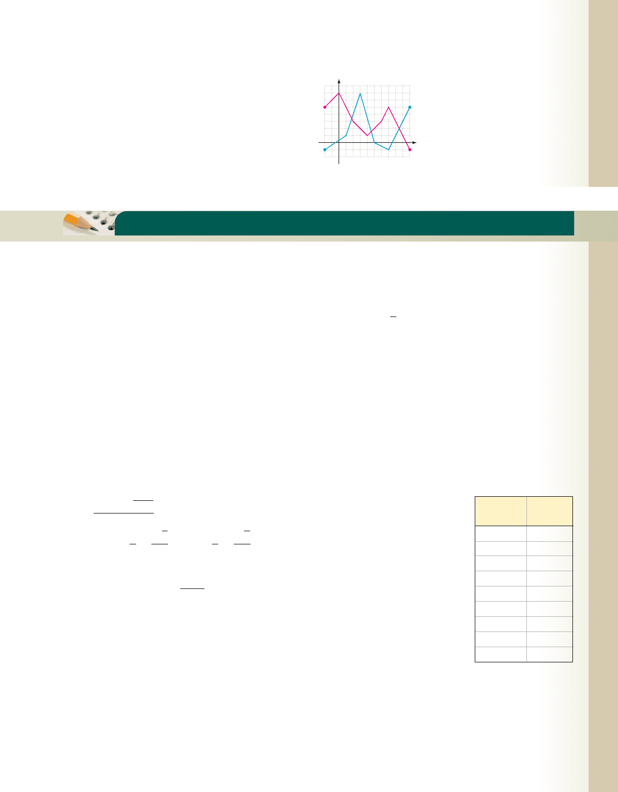
42. Use the graph given to ﬁnd the value of each expression:

43. Use the difference quotient to ﬁnd a rate of change formula for the function given, then calculate the rate of

change for the interval indicated: .j1x2⫽ x

⫺ x; 32.00, 2.014

1f ⴰ g2132

1g ⴰ f 21102

1g ⴰ f 2172

1g ⴰ f 2152

1f ⴰ g21⫺22

105⫺2

⫺2

g(x)

(⫺2, 5)

(⫺2, ⫺1)

f(x)

cob19545_ch03_371-380.qxd 11/25/10 3:56 PM Page 375

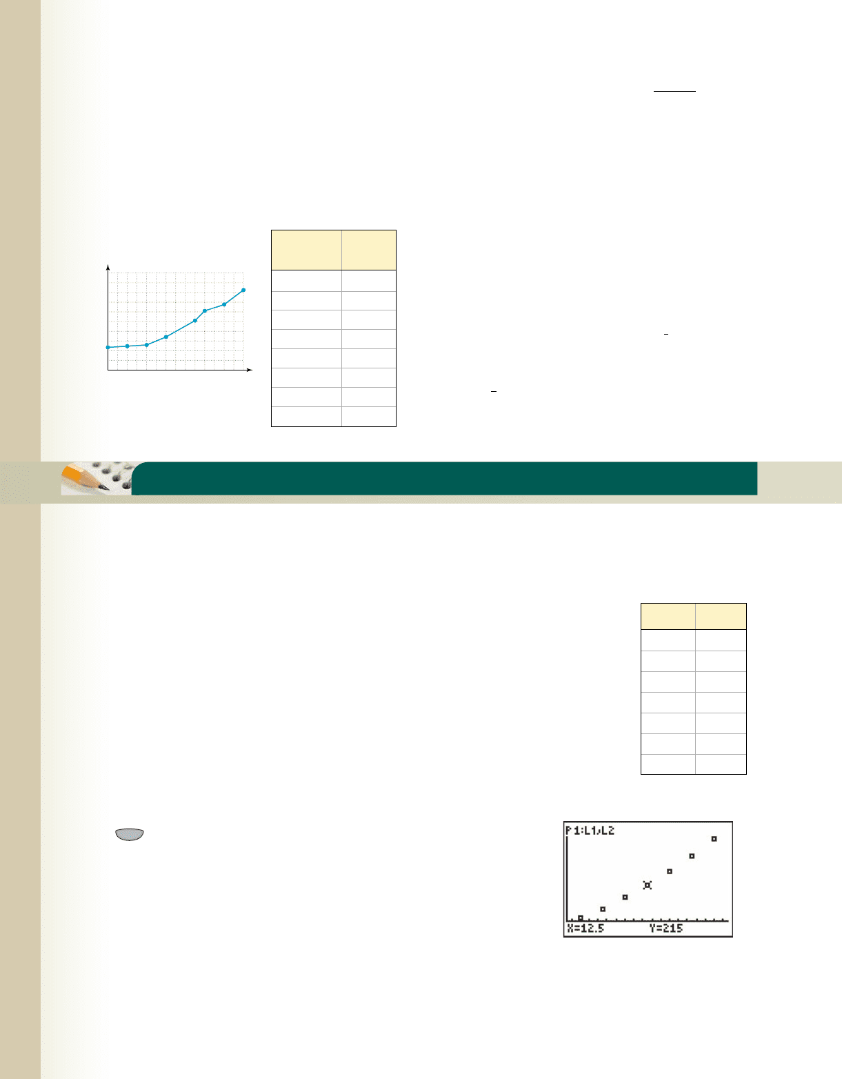
17. The graph and accompanying table show the number

N of new books published in the United States for

selected years t from 1990 to 2004. Find the average

rate of change for the years (a) 1992 to 1996 and

(b) 1996 to 1999. (c) In 1997, the number of new

books published actually fell to 65.8 (1000s). Using

this information, ﬁnd the average rate of change for

the years 1996 to 1997, and 1997 to 1999.

18. Given and ,

determine and its domain.

19. Monthly sales volume for a successful new company

is modeled by , where S(t) represents

sales volume in thousands in month t (

corresponds to January 1). (a) Would you expect

the average rate of change from May to June to be

greater than that from June to July? Why?

(b) Calculate the rates of change in these intervals

to verify your answer. (c) Calculate the difference

quotient for S(t) and use it to estimate the sales

volume rate of change after 10, 18, and 24 months.

20. A snowball increases in size as it rolls downhill. The

snowball is roughly spherical with a radius that can

be modeled by the function where t is

time in seconds and r is measured in inches. The

volume of the snowball is given by the function

Use a composition to (a) write V

directly as a function of t and (b) ﬁnd the volume

of the snowball after 9 sec.

V1r2⫽

␲r

r1t2⫽ 1t

t ⫽ 0

S1t2⫽ 2t

⫺ 3t

1f ⴰ g21x2

g1x2⫽ 13x ⫺ 1

f 1x2⫽ x

⫹ 2

376 CHAPTER 3 Quadratic Functions and Operations on Functions 3–96

College Algebra G&M—

Residuals, Correlation Coefﬁcients, and Goodness of Fit

When using technology to calculate a regression equation, we must avoid relying on the correlation coefﬁcient

as the sole indicator of how well a model ﬁts the data. It is actually possible for a regression to have a high r-value

(correlation coefﬁcient) but ﬁt the data very poorly. In addition, regression models are often used

to predict future values, extrapolating well beyond the given set of data. Sometimes the model

fails miserably when extended—even when it ﬁts the data on the speciﬁed interval very well.

This fact highlights (1) the importance of studying the behavior of the toolbox functions and

other graphs, as we often need to choose between two models that seem to ﬁt the given data;

(2) the need to consider the context of the data; and (3) the need for an additional means to

evaluate the “goodness of ﬁt.” For the third item, we investigate something called a residual.

As the name implies, we are interested in the difference between the outputs generated by the

equation model, and the actual data: equation value data value residual. Residuals that are

fairly random and scattered indicate the equation model has done a good job of capturing the

curvature of the data. If the residuals exhibit a detectable pattern of some sort, this often indicates

trends in the data that the equation model did not account for.

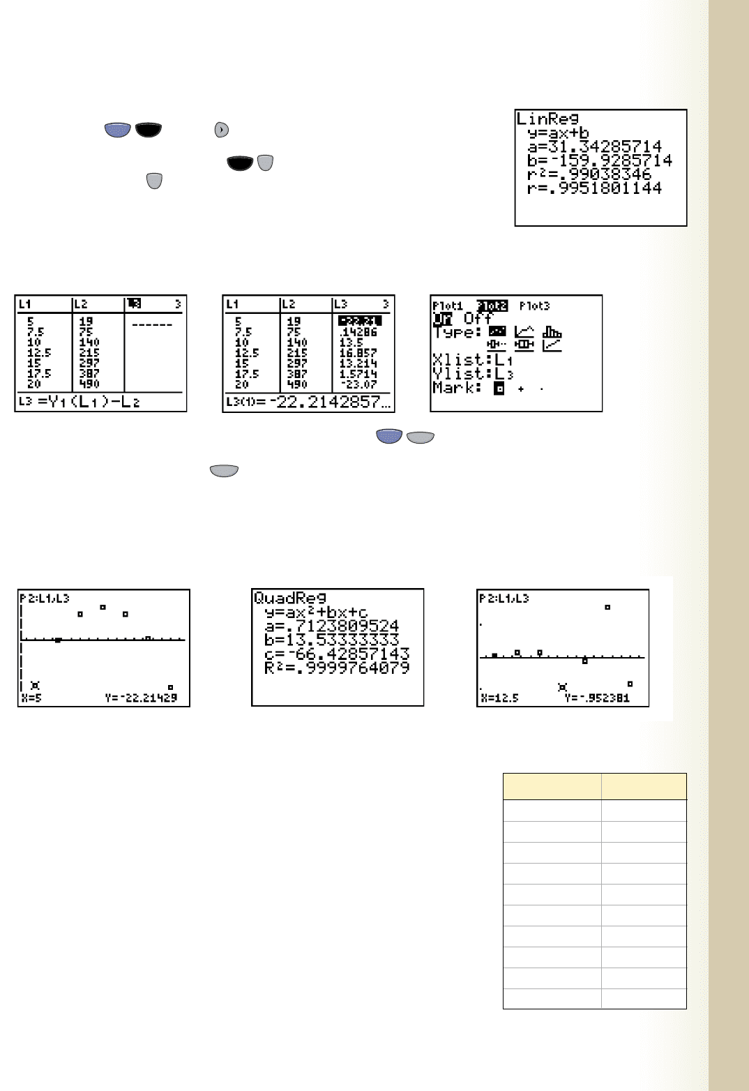
As a simplistic illustration, enter the data from Table 3.5 in L1 and L2,

then graph the scatterplot. Most graphing calculators offer a window option

speciﬁcally designed for scatterplots that will plot the points in an “ideal”

window: 9:ZoomStat (Figure 3.82). Upon inspection, it appears the data

could be linear with positive slope, quadratic with , or some other toolbox

function with increasing behavior. Many of these forms of regression will give a

correlation coefﬁcient in the high 90s. This is where an awareness of the context

is important. (1) Do we expect the data to increase steadily over time (linear

data)? (2) Do we expect the rate of change (the growth rate) to increase over

time (quadratic data)? At what rate will values increase? (3) Do we expect the

growth to increase dramatically with time (power or exponential regression)?

Running a linear regression (LinReg L1, L2, Y

) gives the equation in Figure 3.83, with a very high r-value. This

model appears to ﬁt the data very well, and will reasonably approximate the data points within the interval. But could

we use this model to accurately predict future values (do we expect the outputs to grow indeﬁnitely at a linear rate)?

a 7 0

ZOOM

⫽⫺

21.5

570.07

⫺61.07

3.5

Figure 3.82

Table 3.5

519

7.5 75

10 140

12.5 215

15 297

17.5 387

20 490

CALCULATOR EXPLORATION AND DISCOVERY

Year Books

(1000s)

0 46.7

2 49.2

4 51.7

6 68.2

9 102.0

10 122.1

12 135.1

14 165.8

11990 S 02

Years (1990 → 0)

148642

120

200

160

180

140

100

10 12

Books published (1000s)

cob19545_ch03_371-380.qxd 8/10/10 8:11 PM Page 376

3–97 Calculator Exploration and Discovery 377

College Algebra G&M—

Figure 3.84 Figure 3.85 Figure 3.86

21.5

23.6

⫺29.9

3.5

Figure 3.87

Figure 3.88

21.5

2.00

⫺1.38

3.5

Figure 3.89

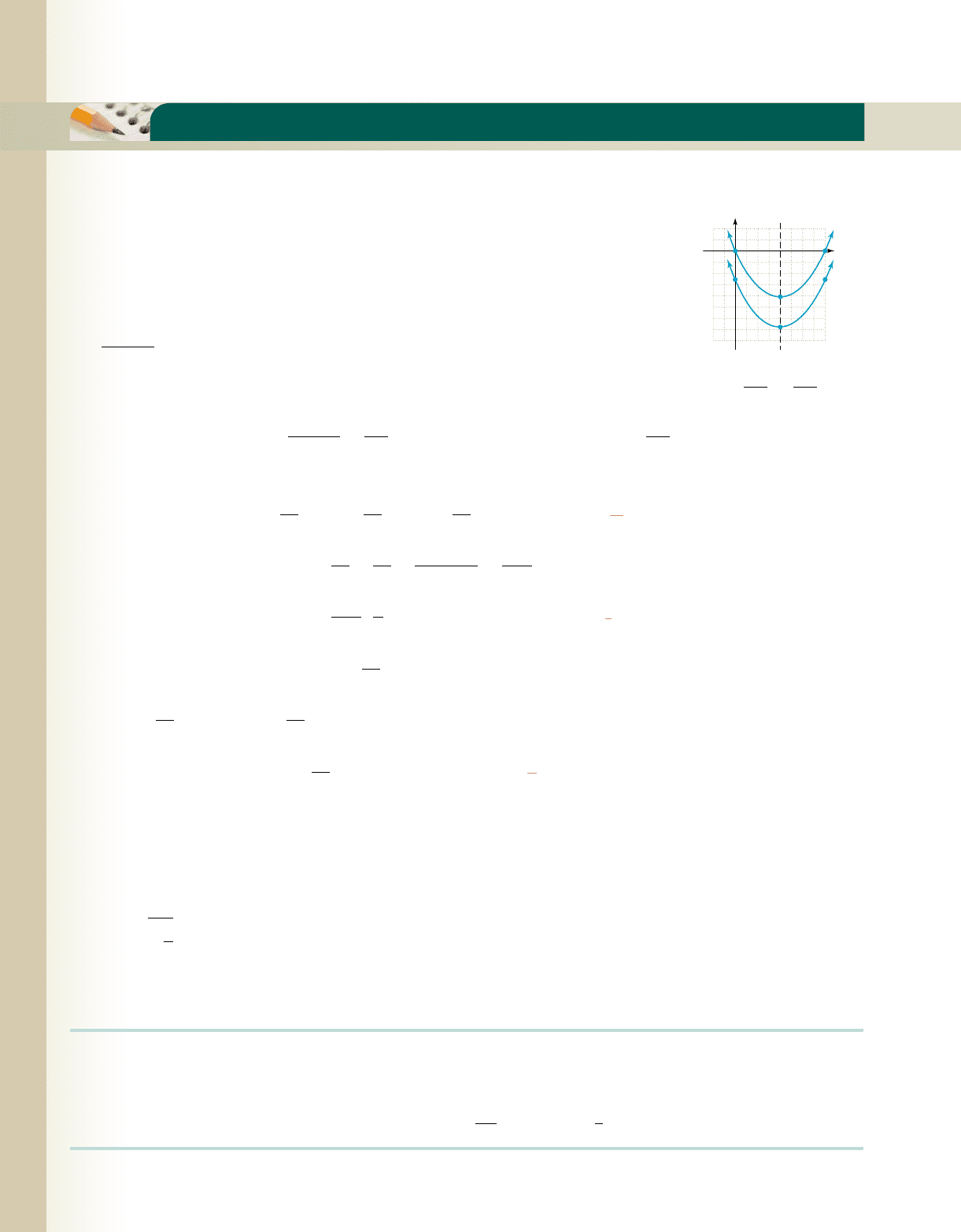
In some cases, the answer will be clear from the context. Other times the decision is

more difﬁcult and a study of the residuals can help. Most graphing calculators provide

a residual function [ (LIST)( )(OPS) 7: List], but to help you

understand more exactly what residuals are, for now we’ll calculate them via function

values. For this calculation, we go to the (EDIT) screen. In the header of L3

(List3), input Y

(L1) L2 (Figure 3.84), which will evaluate the function at the

input values listed in L1, compute the difference between these outputs and the data in

L2, and place the results in L3. Scrolling through the residuals reveals a distinct lack

of randomness, as there is a large interval where outputs are continuously positive

(Figure 3.85).

ENTER

⫺

ENTER

STAT

STAT2nd

We can also analyze the residuals graphically by going to the (STATPLOT) screen to activate

2:PLOT2, setting it up to recognize L1 and L3 as the XList and YList respectively (Figure 3.86). After deactivating

all other plots and functions, pressing 9:ZoomStat gives Figure 3.87 shown, with the residuals following a

deﬁnite (quadratic) pattern. Performing the same sequence of steps using quadratic regression results in a higher

correlation coefﬁcient and an increased randomness in residuals (Figures 3.88 and 3.89), with the residuals appearing

to increase over time.

ZOOM

2nd

Exercise 1: As part of a science lab, students are asked to determine the

relationship between the length of a pendulum and the time it takes to complete

one back-and-forth cycle, called its period. They tie a 500-g weight to 10 different

lengths of string, suspend them from a doorway, and collect the data shown in

Table 3.6.

a. Use a combination of the context, the correlation coefﬁcient, and an analysis of

the residuals to determine whether a linear, quadratic, or power model is most

appropriate for the data. State the r-value of each regression and justify your

ﬁnal choice of equation model.

b. According to the data, what would be the period of a pendulum with a 90-cm

length? A 150-cm length?

c. If the period was 1.6 sec, how long was the pendulum? If the period were 2 sec,

how long was the pendulum?

Table 3.6

Length (cm) Time (sec)

12 0.7

20 0.9

28 1.09

36 1.24

44 1.35

52 1.55

60 1.64

68 1.73

76 1.80

84 1.95

Figure 3.83

cob19545_ch03_371-380.qxd 11/25/10 3:57 PM Page 377

College Algebra G&M—

STRENGTHENING CORE SKILLS

378 CHAPTER 3 Quadratic Functions and Operations on Functions 3–98

Base Functions and Quadratic Graphs

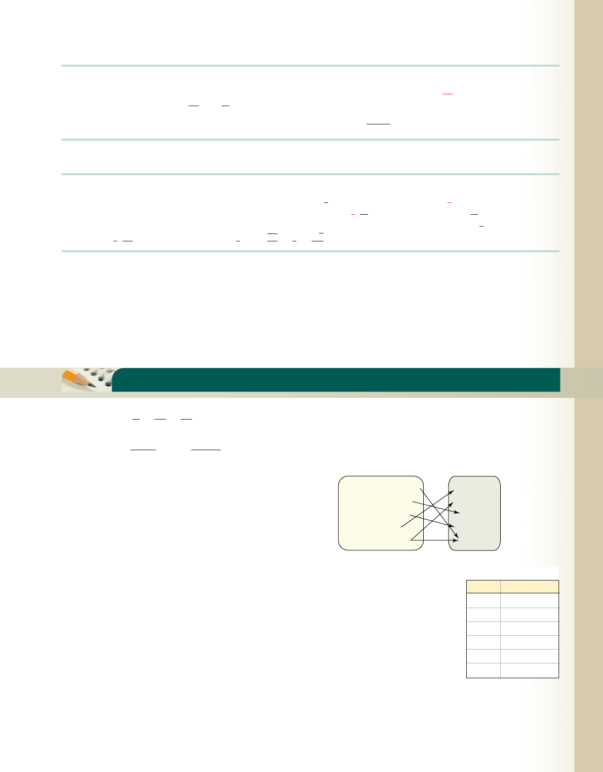
Certain transformations of quadratic graphs offer an intriguing alternative to graphing these

functions by completing the square. In many cases, the process is less time consuming and

ties together a number of basic concepts. To begin, we note that for

is called the base function or the original function less the constant term.

By comparing with four things are immediately apparent: (1) F and f share the

same axis of symmetry since one is a vertical shift of the other; (2) the x-intercepts of F can be

found by factoring; (3) the axis of symmetry is simply the average value of the x-intercepts;

and (4) the vertices of F and f differ only by the constant c. Consider these

vertices to be and (h, k), respectively, with Knowing the vertex of any parabola is we

evaluate the base function at and ﬁnd that for the base function,

original function

substitute for

or multiply and combine terms

multiply by

rearrange factors

From we have and it follows that

substitute

This veriﬁes the vertex of F is , where

It’s signiﬁcant to note that the vertex of both F(x) and f(x) can now be determined using only elementary operations

on the single value h, since and By setting in the quadratic equation

and solving for x

we get the vertex/intercept formula, which can be used to ﬁnd the roots of f with no further calculations:

Finally, this approach enables easy access to the exact form of the roots, even when they happen to

be irrational or complex (no quadratic formula needed). Several examples follow, with the actual graphs left to the

student—only the process is illustrated here.

Illustration 1

䊳

Graph and locate its zeroes (if they exist).

Solution

䊳

For the zeroes/x-intercepts are (0, 0) and (10, 0) by inspection, with (halfway

point) as the axis of symmetry. Noting and , the vertex of F is at or After adding 17

units to the y-coordinates of the points from F, we ﬁnd the y-intercept for f is (0, 17), its “symmetric point” is (10, 17),

and the vertex is at . The x-intercepts of f are or .✓15 ⫾ 18, 021h ⫾ 1⫺k, 0215, ⫺82

15, ⫺252.1h, ⫺ah

2c ⫽ 17a ⫽ 1

h ⫽ 5F1x2⫽ x

⫺ 10x,

1x2⫽ x

⫺ 10x ⫹ 17

x ⫽ h ⫾

⫺

y ⫽ a1x ⫺ h2

⫹ ky ⫽ 0k ⫽ k

⫹ c.k

⫽⫺ah

.1h, k

1⫺h2

⫽ h

⫽⫺ah

⫺h for

F a⫺

b⫽⫺a1⫺h2

⫺h ⫽

h ⫽⫺

⫽⫺aa

⫽

⫺b

⫽

⫺

⫽

⫺ 2b

⫺

F a⫺

b⫽ aa⫺

⫹ ba⫺

F1x2⫽ ax

⫹ bx

⫺b

b⫽⫺ah

:h ⫽

⫹ x

⫽

⫺b

, f a

⫺b

bb,k ⫽ k

⫹ c.1h, k

h ⫽

⫹ x

;

F1x2,f

1x2

1x2⫽ ax

⫹ bx

1x2⫽ ax

⫹ bx ⫹ c,

(0, 0)

(assume a > 0, c < 0)

(0, c)

(h, k

)

(h, k)

冢

⫺

–, 0

冣

冢

⫺

–, c

冣

h, ⫺

—

cob19545_ch03_371-380.qxd 8/10/10 8:12 PM Page 378

College Algebra G&M—

Illustration 2

䊳

Graph and locate its zeroes (if they exist).

Solution

䊳

For the zeroes are (0, 0) and by inspection, with as the axis of symmetry.

Noting and or 12.25, the vertex of F is After subtracting 15 units from

the y-coordinates of the points from F, we ﬁnd the y-intercept for f is its “symmetric point” is

and the vertex is at The x-intercepts of f are ✓

Even when the method lends a measure of efﬁciency to graphing quadratic functions, as shown in Illustration 3.

Illustration 3

䊳

Graph and locate its zeroes (if they exist).

Solution

䊳

For the zeroes are (0, 0) and by inspection, with as the halfway point and

axis of symmetry. Noting and , the vertex of F is at . After subtracting units from the

y-coordinates of the points from F, we ﬁnd the y-intercept for f is its “symmetric point” is and the

vertex is at The roots of f are ✓, showing the graph has no x-intercepts.

Use this method for graphing quadratic functions to sketch a complete graph of the following functions. Find and

clearly indicate the axis of symmetry, vertex, x-intercept(s), and the y-intercept along with its “symmetric point.”

Exercise 1: Exercise 2:

Exercise 3: Exercise 4:

Exercise 5: Exercise 6: q1x2⫽ 2x

⫺ 7x ⫹ 8p1x2⫽ 2x

⫹ 12x ⫹ 21

H1x2⫽⫺x

⫹ 10x ⫺ 17h1x2⫽ x

⫺ 6x ⫹ 11

g1x2⫽ x

⫹ 5x ⫹ 9f 1x2⫽ x

⫹ 2x ⫺ 7

x ⫽

⫾ 2

⫺7

⫽

⫾

⫺7

, ⫺42,10, ⫺42,

4 ⫽

2c ⫽⫺4a ⫽⫺2

h ⫽

, 02F 1x2⫽⫺2x

⫹ 5x,

1x2⫽⫺2x

⫹ 5x ⫺ 4

a ⫽ 1

1⫺3.5 ⫾ 127.25

, 02.1⫺3.5, ⫺27.252.

1⫺7, ⫺152,10, ⫺152,

1⫺3.5, ⫺12.252.1

⫺7

⫽

a ⫽ 1, c ⫽⫺15,

h ⫽

⫺7

1⫺7, 02F1x2⫽ x

⫹ 7x,

1x2⫽ x

⫹ 7x ⫺ 15

3–99 Cumulative Review Chapters R–3 379

CUMULATIVE REVIEW CHAPTERS R–3

1. Solve for

2. Solve for

3. Factor the expressions:

a. b.

4. Solve using the quadratic formula. Write answers in

both exact and approximate form:

5. Solve the following inequality: or

6. Name the eight toolbox functions, give their

equations, then draw a sketch of each.

7. Use substitution to verify that is a

solution to

8. Given and ﬁnd:

and

9. As part of a study on trafﬁc conditions, the mayor of

a small city tracks her driving time to work each day

for six months and ﬁnds a linear and increasing

relationship. On day 1, her drive time was 17 min.

By day 61 the drive time had increased to 28 min.

Find a linear function that models the drive time and

1g ⴰ f 21⫺22.1f ⫼ g21x2,1f

g21x2,

g1x2⫽ x ⫺ 2f

1x2⫽ 3x

⫺ 6x

⫺ 4x ⫹ 13 ⫽ 0.

x ⫽ 2 ⫺ 3i

5 ⫺ x 6 4.

x ⫹ 3 6 5

⫹ 4x ⫹ 1 ⫽ 0.

⫺ 3x

⫺ 4x ⫹ 12x

⫺ 1

x ⫹ 1

⫹ 1 ⫽

⫺ 1

⫽

⫹

use it to estimate the drive time on day 121, if the

trend continues. Explain what the slope of the line

means in this context.

10. Does the relation shown represent a function? If not,

discuss/explain why not.

11. The data given shows the

proﬁt of a new company

for the ﬁrst 6 months of

business, and is closely

modeled by the function

where p(m) is the proﬁt

earned in month m. Assuming

this trend continues, use

this function to ﬁnd the

ﬁrst month a proﬁt will be

earned .

1p 7 02

p1m2⫽1.18x

⫺ 10.99x ⫹ 4.6,

Jackie Joyner-Kersee

Sarah McLachlan

Hillary Clinton

Sally Ride

Venus Williams

Astronaut

Tennis Star

Singer

Politician

Athlete

Exercise 11

Month Proﬁt (1000s)

6 ⫺19

⫺21

⫺20

⫺18

⫺13

⫺5

cob19545_ch03_371-380.qxd 8/10/10 8:12 PM Page 379