Chow T.L. Mathematical Methods for Physicists: A Concise Introduction
Подождите немного. Документ загружается.

We assume that
; '; zR'Zz: 10 :16
Substitution into Eq. (10.15) yields, after division by ,
1
R
d
d
dR
d
1
2
d
2
d'
2
ÿ
1
Z
d
2
Z
dz
2
: 10:17
Clearly, both sides of Eq. (10.17) must be equal to a con stant, say ÿk
2
. Then
1
Z
d
2
Z
dz
2
k
2
or
d
2
Z
dz
2
ÿ k
2
Z 0 10:18
and
1
R
d
d
dR
d
1
2
d
2
d'
2
ÿk
2
or
R
d
d
dR
d
k
2
2
ÿ
1
d
2
d'
2
:
Both sides of this last equation must be equal to a constant, say
2
. Hence
d
2
d'
2
2
0; 10:19
1
R
d
d
dR
d
k
2
ÿ
2
2
þ!
R 0: 10:20
Equation (10.18) has for solutions
Zz
cke
kz
c
0
ke
ÿkz
; k 6 0; 0 < k < 1;
c
1
z c
2
; k 0;
(
10:21
where c and c
0
are arbitrary functions of k and c
1
and c
2
are arbitrary constants.
Equation (10.19) has solutions of the form
'
ae
i'
;6 0; ÿ1 <<1;
b' b
0
; 0:
(
That the potential must be single-valued requires that '' 2n, where
n is an integ er. It follows from this that must be an integer or zero and that
b 0. Then the solution ' becomes
'
ae
i'
a
0
e
ÿi'
;6 0; intege r;
b
0
; 0:
(
10:22
396
PARTIAL DIFFERENTIAL EQUATIONS

In the special case k 0, Eq. (10.20) has solutions of the form
R
d
d
0
ÿ
;6 0;
f ln g; 0:
10:23
When k 6 0, a simple change of variable can put Eq. (10.20) in the form of
Bessel's equation. Let x k, then dx kd and Eq. (10.20) becomes
d
2
R
dx
2
1
x
dR
dx
1 ÿ
2
x
2
þ!
R 0; 10:24
the well-known Bessel's equation (Eq. (7.71)). As shown in Chapter 7, Rx can be
written as
RxAJ
xBJ
ÿ
x; 10:25
where A and B are constants, and J
x is the Bessel function of the ®rst kind.
When is not an integer, J
and J
ÿ
are independent. But when is an integer,
J
ÿ
xÿ1
n
J
x, thus J
and J
ÿ
are linearly dependent, and Eq. (10.25)
cannot be a general solution. In this case the general solution is given by
RxA
1
J
xB
1
Y
x; 10:26
where A
1
and B
2
are constants; Y
x is the Bessel function of the second kind of
order or Neumann's function of order N
x.
The general solution of Eq. (10.20) when k 6 0 is therefore
RpJ
kqY
k; 10:27
where p and q are arbitrary functions of . Then these functions are also solu-
tions:
H
1
kJ
kiY
k; H
2
kJ
kÿiY
k:
These are the Hankel functions of the ®rst and second kinds of order , respec-
tively.
The functions J
; Y
(or N
), and H
1
,andH
2
which satisfy Eq. (10.20) are
known as cylindrical functions of integral order and are denoted by Z
k,
which is not the same as Zz. The solution of Laplace's equation (10.15) can now
be written
; '; z
c
1
z bf ln g ; k 0; 0;
c
1
z bd
d
0
ÿ
ae
i'
a
0
e
ÿi'
;
k 0;6 0;
cke
kz
c
0
ke
ÿkz
Z
0
k; k 6 0; 0;
cke
kz
c
0
ke
ÿkz
Z
kae
i'
a
0
e
ÿi'
; k 6 0 ;6 0:
8
>
>
>
>
>
>
<
>
>
>
>
>
>
:
397
SOLUTIONS OF LAPLACE'S EQUATION
Let us now apply the solutions of Laplace's equation in cylindrical coordinates
to an in®nitely long cylindrical conductor with radius l and charge per unit length
. We want to ®nd the potential at a point P a distance >l from the axis of the
cylindrical. Take the origi n of the coordinates on the axis of the cylinde r that is
taken to be the z-axis. The surface of the cylinder is an equipotential:
lconst: for r l and all ' and z:
The secondary boundary condition is that
E ÿ@=@ =2l" for r l and all ' and z:
Of the four types of solutions to Laplace's equation in cylindrical coordinates
listed above only the ®rst can satisfy these two boundary conditions. Thus
bf ln gÿ
2"
ln
l
a:
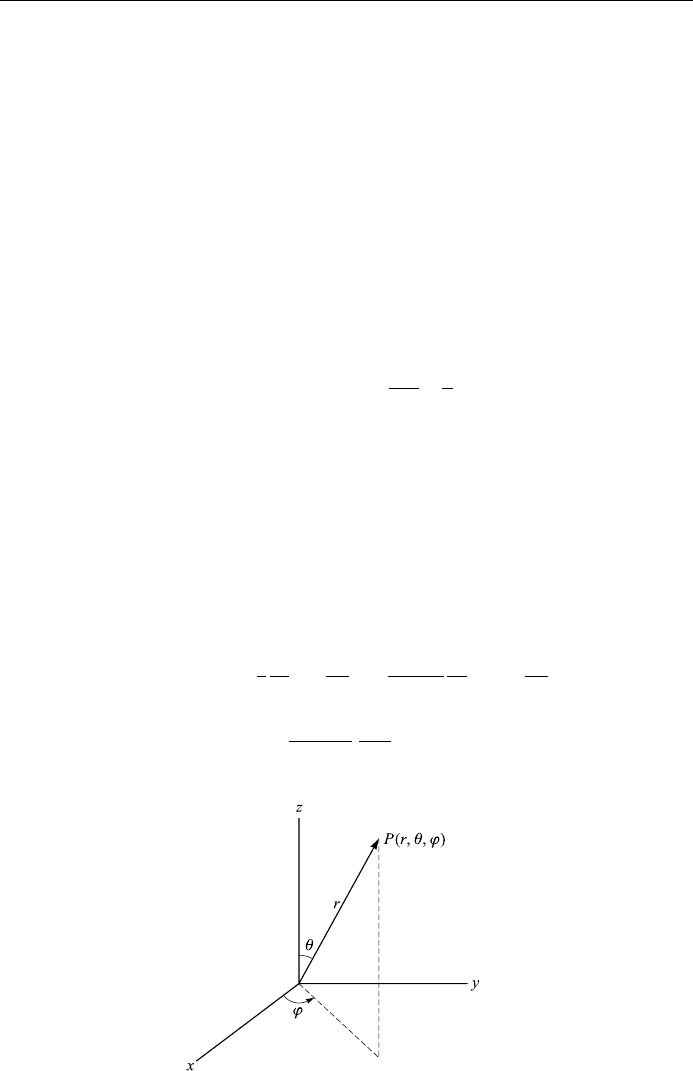
(4) Laplace's equ ation in spherical coordinates r;;': The spherical coordinates
are shown in Fig. 10.2, where
x r sin cos ';
y r sin sin ';
z r cos ':
Laplace's equation now reads
r
2
r;;'
1
r
@
@r
r
2
@
@r
1
r
2
sin
@
@
sin
@
@
1
r
2
sin
2
@
2
@'
2
0:
10:28
398
PARTIAL DIFFERENTIAL EQUATIONS
Figure 10.2. Spherical coordinates.
Again, assume that
r;;'Rr': 10:29
Substituting into Eq. (10.28) and dividing by we obtain
sin
2
R
d
dr
r
2
dR
dr
sin
d
d
sin
d
d
ÿ
1
d
2
d'
2
:
For a solution, both sides of this last equation must be equal to a constant, say
m
2
. Then we have two equations
d
2
d'
2
m
2
0; 10:30
sin
2
R
d
dr
r
2
dR
dr
sin
d
d
sin
d
d
m
2
;
the last equation can be rewritten as
1
sin
d
d
sin
d
d
ÿ
m
2
sin
2
ÿ
1
R
d
dr
r
2
dR
dr
:
Again, both sides of the last equation must be equal to a constant, say ÿÿ. This
yields two equations
1
R
d
dr
r
2
dR
dr
ÿ; 10:31
1
sin
d
d
sin
d
d
ÿ
m
2
sin
2
ÿÿ:
By a simple substitution: x cos , we can put the last equation in a more familiar
form:
d
dx
1 ÿ x
2
dP
dx
ÿ ÿ
m
2
1 ÿ x
2
þ!
P 0 10:32
or
1 ÿ x
2
d
2
P
dx
2
ÿ 2x
dP
dx
ÿ ÿ
m
2
1 ÿ x
2
"#
P 0; 10: 32a
where we have set Px.
You may have already noticed that Eq. (10.32) is very similar to Eq. (10.25),
the associated Legendre equation. Let us take a close look at this resemblance.
In Eq. (10.32), the points x 1 are regular singular points of the equation. Let
us ®rst study the behavior of the solution near point x 1; it is convenient to
399
SOLUTIONS OF LAPLACE'S EQUATION
bring this regular singular point to the origin, so we make the substitution
u 1 ÿ x; UuPx. Then Eq. (10.32) becomes
d
du
u2 ÿ u
dU
du
ÿ ÿ
m
2
u2 ÿ u
"#
U 0:
When we solve this equation by a power series: U
P
1
n0
a
n
u
n
, we ®nd that the
indicial equation leads to the values m=2 for . For the point x ÿ1, we make
the substitution v 1 x, and then solve the resulting diÿerential equation by the
power series method; we ®nd that the indicial equation leads to the same values
m=2 for .
Let us ®rst consider the value m=2; m 0. The above considerations lead us
to assume
Px1 ÿ x
m=2
1 x
m=2
yx1 ÿ x
2
m=2
yx; m 0
as the solution of Eq. (10.32). Substituting this into Eq. (10.32) we ®nd
1 ÿ x
2
d
2
y
dx
2
ÿ 2m 1x
dy
dx
ÿ ÿ mm 1y 0 :
Solving this equation by a power series
yx
X
1
n0
c
n
x
n
;
we ®nd that the indicial equation is ÿ 10. Thus the solution can be written
yx
X
n even
c
n
x
n
X
n odd
c
n
x
n
:
The recursion formula is
c
n2
n mn m 1ÿÿ
n 1n 2
c
n
:
Now consider the convergence of the series. By the ratio test,
R
n
c
n
x
n
c
nÿ2
x
nÿ2
ÿ
ÿ
ÿ
ÿ
ÿ
ÿ
ÿ
ÿ
n mn m 1ÿÿ
n 1n 2
ÿ
ÿ
ÿ
ÿ
ÿ
ÿ
ÿ
ÿ
x
jj
2
:
The series converges for jxj < 1, whatever the ®nite value of ÿ may be. For
jxj1, the ratio test is inconclusive. However, the integral test yields
Z
M
t mt m 1ÿÿ
t 1t 2
dt
Z
M
t mt m 1
t 1t 2
dt ÿ
Z
M
ÿ
t 1t 2
dt
and since
Z
M
t mt m 1
t 1t 2
dt !1 as M !1;
400
PARTIAL DIFFERENTIAL EQUATIONS
the series diverges for jxj1. A solution which converges for all x can be
obtained if either the even or odd series is terminated at the term in x
j
. This
may be done by setting ÿ equal to
ÿ j mj m 1ll 1:
On substituting this into Eq. (10.32a), the resulting equation is
1 ÿ x
2
d
2
P
dx
2
ÿ 2x
dP
dx
ll 1ÿ
m
2
1 ÿ x
2
"#
P 0;
which is identical to Eq. (7.25). Special solutions were studied there: they were
written in the form P
m
l
x and are known as the associated Legendre functions of
the ®rst kind of degree l and order m, where l and m, take on the values
l 0; 1; 2; ...; and m 0; 1; 2; ...; l. The general solution of Eq. (10.32) for
m 0 is therefore
Pxa
l
P
m
l
x: 10:33
The second solution of Eq. (10.32) is given by the associated Legendre function of
the second kind of degree l and order m: Q
m
l
x. However, only the associated
Legendre function of the ®rst kind remains ®ni te over the range ÿ1 x 1 (or
0 2.
Equation (10.31) for Rr becomes
d
dr
r
2
dR
dr
ÿ ll 1R 0: 10:31a
When l 6 0, its solution is
Rrblr
l
b
0
lr
ÿlÿ1
; 10:34
and when l 0, its solution is
Rrcr
ÿ1
d: 10 :35
The solution of Eq. (10.30) is
f me
im'
f
0
le
ÿim'
; m 6 0; positive integer;
g; m 0:
(
10:36
The solution of Laplace's equation (10.28) is therefore given by
r;;'
br
l
b
0
r
ÿlÿ1
P
m
l
cos fe
im'
f
0
e
ÿim'
; l 6 0; m 6 0;
br
l
b
0
r
ÿlÿ1
P
l
cos ; l 6 0; m 0;
cr
ÿ1
dP
0
cos ; l 0; m 0;
8
>
<
>
:
10:37
where P
l
P
0
l
.
401
SOLUTIONS OF LAPLACE'S EQUATION
We now illustrate the usefulness of the above result for an electrostatic problem
having spherical symmetry. Consider a conducting spherical shell of radius a and
charge per unit area. The problem is to ®nd the potential r;;' at a point P a
distance r > a from the center of shell. Take the origin of co ordinates to be at the
center of the shell. As the surface of the shell is an equipotential, we have the ®rst
boundary condition
rconstant a for r a and all and ': 10:38
The second boundary condition is that
! 0 for r !1and all and ': 10:39
Of the three types of solutions (10.37) only the last can satisfy the boundary
conditions. Thus
r;;'cr
ÿ1
dP
0
cos : 10 :40
Now P
0
cos 1, and from Eq. (10.38) we have
aca
ÿ1
d:
But the boundary condition (10.39) requires that d 0. Thus aca
ÿ1
,or
c aa, and Eq. (10.40) reduces to
r
aa
r
: 10:41
Now
a=a EaQ=4a
2
";
where " is the permittivity of the dielectric in which the shell is embedded,
Q 4a
2
. Thus aa=", and Eq. (10.41) becomes
r
a
2
"r
: 10:42
Solutions of the wave equation: separation of variables
We now use the method of separation of variables to solve the wave equation
@
2
ux; t
@x
2
v
ÿ2
@
2
ux; t
@t
2
; 10:43
subject to the following boundary conditions:
u0; tul; t0; t 0; 10 :44
ux; 0f t; 0 x l; 10 :45
402
PARTIAL DIFFERENTIAL EQUATIONS
and
@ux; t
@t
ÿ
ÿ
ÿ
ÿ
t0
gx; 0 x l; 10:46
where f and g are given functions.
Assuming that the solution of Eq. (10.43) may be written as a product
ux; tXxT t; 10:47
then substituting into Eq. (10.43) and dividing by XT we obtain
1
X
d
2
X
dx
2
1
v
2
T
d
2
T
dt
2
:
Both sides of this last equation must be equal to a constant, say ÿb
2
=v
2
. Then we
have two equations
1
X
d
2
X
dx
2
ÿ
b
2
v
2
; 10:48
1
T
d
2
T
dt
2
ÿb
2
: 10:49
The solutions of these equations are periodic, and it is more convenient to write
them in terms of trigonometric functions
XxA sin
bx
v
B cos
bx
v
; TtC sin bt D cos bt; 10:50
where A; B; C, and D are arbitrary constants, to be ®xed by the boundary condi-
tions. Equation (10.47) then becomes
ux; t A sin
bx
v
B cos
bx
v
C sin bt D cos bt: 10:51
The boundary condition u0; t0t > 0 gives
0 BC sin bt D cos bt
for all t, which implies
B 0: 10:52
Next, from the boundary condition ul; t0t > 0 we have
0 A sin
bl
v
C sin bt D cos bt:
Note that B 0 would make u 0. However, the last equation can be satis®ed
for all t when
sin
bl
v
0;
403
SOLUTIONS OF LAPLACE'S EQUATION
which impl ies
b
nv
l
; n 1; 2; 3; ...: 10:53
Note that n cannot be equal to zero, because it would make b 0, which in turn
would mak e u 0.
Substituting Eq. (10.53) into Eq. (10.51) we have
u
n
x; tsin
nx
l
C
n
sin
nvt
l
D
n
cos
nvt
l
; n 1 ; 2; 3; ...: 10:54
We see that there is an in®nite set of discrete values of b and that to each value of
b there corresponds a particular solution. Any linear combination of these parti-
cular solutions is also a solution:
u
n
x; t
X
1
n1
sin
nx
l
C
n
sin
nvt
l
D
n
cos
nvt
l
: 10:55
The constants C
n
and D
n
are ®xed by the boundary conditions (10.45) and
(10.46).
Application of boundary condition (10.45) yields
f x
X
1
n1
D
n
sin
nx
l
: 10:56
Similarly, application of boundary condition (10.46) gives
gx
v
l
X
1
n1
nC
n
sin
nx
l
: 10:57
The coecients C
n
and D
n
may then be determined by the Fourier series method:
D
n
2
l
Z
l
0
f xsin
nx
l
dx; C
n
2
nv
Z
l
0
gxsin
nx
l
dx: 10:58
We can use the method of separation of varia ble to solve the heat conduction
equation. W e shall leave this as a home work problem.
In the following sections, we shall consider two more methods for the solution
of linear partial diÿerential equations: the method of Green's functions, and the
method of the Laplace transformation which was used in Chapter 9 for the
solution of ordinary linear diÿerential equations with constant coecients.
Solution of Poisson's equation. Green's functions
The Green's function approach to boundary-value problems is a very powerful
technique. The ®eld at a point caused by a source can be considered to be the total
eÿect due to each ``unit'' (or elementary portion) of the source. If Gx; x
0
is the
404
PARTIAL DIFFERENTIAL EQUATIONS

®eld at a point x due to a unit point source at x
0
, then the total ®eld at x due to a
distributed source x
0
is the integral of G over the range of x
0
occupied by the
source. The function Gx; x
0
is the well-known Green's function. We now apply
this technique to solve Poisson's equation for electric potential (Example 10.2)
r
2
rÿ
1
"
r; 10:59
where is the charge density and " the permittivity of the medium, both are given.
By de®nition, Green's function Gr; r
0
is the solution of
r
2
Gr; r
0
r ÿ r
0
; 10:60
where r ÿ r
0
is the Dirac delta function.
Now, multiplying Eq. (10.60) by and Eq. (10.59) by G, and then subtracting,
we ®nd
rr
2
Gr; r
0
ÿGr; r
0
r
2
rrr ÿ r
0
1
"
Gr; r
0
r;
and on interchanging r and r
0
,
r
0
r
02
Gr
0
; rÿGr
0
; rr
02
r
0
r
0
r
0
ÿ r
1
"
Gr
0
; rr
0
or
r
0
r
0
ÿ rr
0
r
02
Gr
0
; rÿGr
0
; rr
02
r
0
ÿ
1
"
Gr
0
; rr
0
; 10:61
the prime on r indicates that diÿerentiation is with respect to the primed co-
ordinates. Integrating this last equation over all r
0
within and on the surface S
0
which encloses all sources (charges) yields
rÿ
1
"
Z
Gr; r
0
r
0
dr
0
Z
r
0
r
02
Gr; r
0
ÿGr; r
0
r
02
r
0
dr
0
; 10:62
where we have used the property of the delta function
Z
1
ÿ1
f r
0
r ÿ r
0
dr
0
f r:
We now use Green's theorem
ZZZ
f r
02
þ ÿ þr
02
f d
0
ZZ
f r
0
þ ÿ þr
0
f dS
405
SOLUTIONS OF POISSON'S EQUATION