Chow T.L. Mathematical Methods for Physicists: A Concise Introduction
Подождите немного. Документ загружается.

From Eq. (7.76a) we obtain J
0
0
as
J
0
0
x
X
1
m1
ÿ1
m
2mx
2mÿ1
2
2m
m!
2
X
1
m1
ÿ1
m
x
2mÿ1
2
2mÿ1
m!m ÿ 1!
:
By inserting this series we have
X
1
m1
ÿ1
m
x
2mÿ1
2
2mÿ2
m!m ÿ 1!
X
1
m1
m
2
A
m
x
mÿ1
X
1
m1
A
m
x
m1
0:
We ®rst show that A
m
with odd subscripts are all zero. The coecient of the
power x
0
is A
1
and so A
1
0. By equating the sum of the coecients of the power
x
2s
to zero we obtain
2s 1
2
A
2s1
A
2sÿ1
0; s 1; 2; ...:
Since A
1
0, we thus obtain A
3
0; A
5
0; ...; successively. We now equate the
sum of the coecients of x
2s1
to zero. For s 0 this gives
ÿ1 4A
2
0orA
2
1=4:
For the other values of s we obtain
ÿ1
s1
2
s
s 1!s!
2s 2
2
A
2s2
A
2s
0:
For s 1 this yields
1=8 16A
4
A
2
0orA
4
ÿ3=128
and in general
A
2m
ÿ1
mÿ1
2
m
m!
2
1
1
2
1
3
1
m
; m 1; 2; ...: 7 :82
Using the short notation
h
m
1
1
2
1
3
1
m
and inserting Eq. (7.82) and A
1
A
3
0 into Eq. (7.81) we obtain the result
y
2
xJ
0
xln x
X
1
m1
ÿ1
mÿ1
h
m
2
2m
m!
2
x
2m
J
0
xln x
1
4
x
2
ÿ
3
128
x
4
ÿ: 7:83
Since J
0
and y
2
are linearly independent functions, they form a fundamental
system of Eq. (7.80). Of course, another fundamental system is obtained by
replacing y
2
by an independent particular solution of the form ay
2
bJ
0
,
where a6 0 and b are constant s. It is customary to choo se a 2= and
326
SPECIAL FUNCTIONS OF MATHEMATICAL PHYSICS
b ÿ ÿ ln 2, where ÿ 0:577 215 664 90 ... is the so-called Euler constant, which
is de®ned as the limit of
1
1
2
1
s
ÿ ln s
as s approaches in®nity. The standard particular solution thus obtained is known
as the Bessel function of the second kind of order zero or Neumann's function of
order zero and is denoted by Y
0
x:
Y
0
x
2
J
0
x ln
x
2
ÿ
X
1
m1
ÿ1
mÿ1
h
m
2
2m
m!
2
x
2m
: 7:84
If 1; 2; ...; a second solution can be obtained by similar manipulations,
starting from Eq. (7.35). It turns out that in this case also the solution contains a
logarithmic term. So the second solution is unbounded near the origin and is
useful in applications only for x 6 0.
Note that the second solution is de®ned diÿerently, depending on whether the
order is integral or not. To provide uniformity of formalism and numeri cal
tabulation, it is desirable to adopt a form of the second solution that is valid for
all values of the order. The common choice for the standard second solution
de®ned for all is given by the formula
Y
x
J
xcos ÿ J
ÿ
x
sin
; Y
n
xlim
!n
Y
x: 7:85
This function is known as the Bessel function of the second kind of order .Itis
also known as Neumann's function of order and is denoted by N
x (Carl
Neumann 1832±1925, Germ an mathematician and physicist) . In G. N. Watson's
A Treatise on the Theory of Bessel Functi ons (2nd ed. Cambridge University Press,
Cambridge, 1944), it was called Weber's function and the notation Y
x was
used. It can be shown that
Y
ÿn
xÿ1
n
Y
n
x:
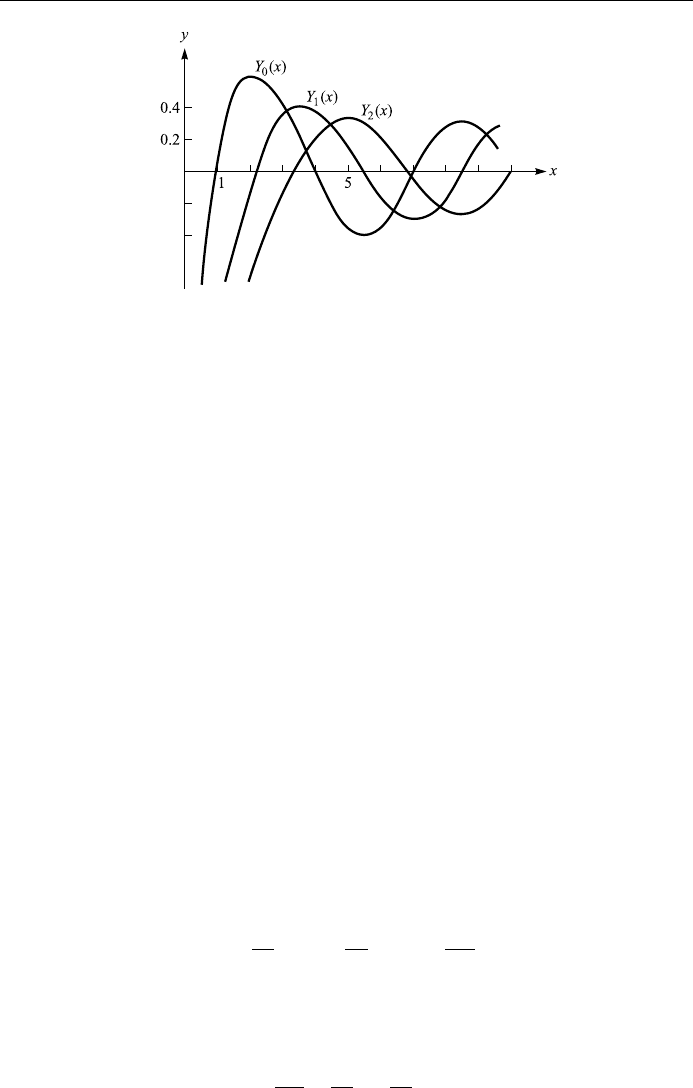
We plot the ®rst three Y
n
x in Fig. 7.4.
A general solution of Bessel's equation for all values of can now be written:
yxc
1
J
xc
2
Y
x:
In some applications it is convenient to use solutions of Bessel's equation that
are complex for all values of x, so the following solutions were intro duced
H
1
xJ
xiY
x;
H
2
xJ
xÿiY
x:
9
=
;
7:86
327
BESSEL'S EQUATION
These linearly independent functions are known as Bessel functions of the third
kind of order or ®rst and second Hankel functions of order (Hermann
Hankel, 1839±1873, German mathematician).
To illustrate how Bessel functions enter into the analysis of physical problems,
we consider one example in classical physics: small oscillations of a hanging chain,
which was ®rst considered as early as 1732 by Daniel Bernoulli.
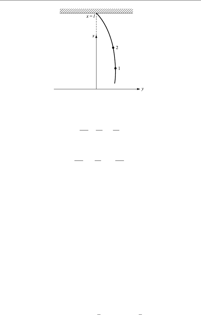
Hanging ¯exible chain
Fig. 7.5 shows a uniform heavy ¯exible chain of length l hanging vertically under
its own weight. The x-axis is the position of stable equilibrium of the chain and its
lowest end is at x 0. We consider the problem of small oscillations in the vertical
xy plane caused by small displacements from the stable eq uilibrium position. This
is essentially the problem of the vibrating string which we discussed in Chapter 4,
with two important diÿerences: here, instead of being constant, the tension T at a
given point of the chain is equal to the weight of the chain below that point, and
now one end of the chain is free, whereas before both ends were ®xed. The
analysis of Chapter 4 generally holds. To derive an equation for y, consider an
element dx, then Newton's second law gives
T
@y
@x
2
ÿ T
@y
@x
1
dx
@
2
y
@t
2
or
dx
@
2
y
@t
2
@
@x
T
@y
@x
dx;
328
SPECIAL FUNCTIONS OF MATHEMATICAL PHYSICS
Figure 7.4. Bessel functions of the second kind.
from which we obtain
@
2
y
@t
2
@
@x
T
@y
@x
:
Now T gx. Substituting this into the above equation for y, we obtain
@
2
y
@t
2
g
@y
@x
gx
@
2
y
@x
2
;
where y is a function of two variables x and t. The ®rst step in the solut ion is to
separate the variables. Let us attempt a solution of the form yx; tuxf t.
Substitution of this into the partial diÿerential equation yields two equations:
f
00
t!
2
f t0; xu
00
xu
0
x!
2
=gux0;
where !
2
is the separation constant. The diÿerential equation for f t is ready for
integration and the result is f tcos!t ÿ , with a phase constant. The
diÿerential equation for ux is not in a recognizable form yet. To solve it, ®rst
change variables by putting
x gz
2
=4; wzux;
then the diÿerential equation for ux becomes Bessel's equation of order zero:
zw
00
zw
0
z!
2
zwz0:
Its general solution is
wzAJ
0
!zBY
0
!z
or
uxAJ
0
2!
x
g
r
BY
0
2!
x
g
r
:
329
BESSEL'S EQUATION
Figure 7.5. A ¯exible chain.

Since Y
0
2!
x=g
p
!ÿ1as x ! 0, we are forced by physics to choose B 0
and then
yx; tAJ
0
2!
x
g
r
cos!t ÿ :
The upper end of the chain at x l is ®xed, requiring that
J
0
2!
`
g
s
ý!
0:
The frequenci es of the normal vibrations of the chain are given by
2!
n
`
g
s
n
;
where
n
are the roots of J
0
. Som e values of J
0
x and J
1
x are tabulated at the
end of this chapter.
Generating function for J
n
x
The function
x; te
x=2tÿt
ÿ1
X
1
nÿ1
J
n
xt
n
7:87
is called the generating function for Bessel functions of the ®rst kind of integral
order. It is very useful in obtaining properties of J
n
x for integral values of n
which can then often be proved for all values of n.
To prove Eq. (7.87), let us consider the exponential functions e
xt=2
and e
ÿxt=2
.
The Laurent expansions for these two exponential functions about t 0 are
e
xt=2
X
1
k0
xt=2
k
k!
; e
ÿxt=2
X
1
m0
ÿxt=2
k
m!
:
Multiplying them together, we get
e
xtÿt
ÿ1
=2
X
1
k0
X
1
m0
ÿ1
m
k!m!
x
2
km
t
kÿm
: 7:88
It is easy to recognize that the coecient of the t
0
term which is made up of those
terms with k m is just J
0
x:
X
1
k0
ÿ1
k
2
2k
k!
2
x
2k
J
0
x:
330
SPECIAL FUNCTIONS OF MATHEMATICAL PHYSICS

Similarly, the coecient of the term t
n
which is made up of those terms for
which k ÿ m n is just J
n
x:
X
1
k0
ÿ1
k
k n!k!2
2kn
x
2kn
J
n
x:
This shows clearly that the coecients in the Laurent expansion (7.88) of the
generating function are just the Bessel functions of integral order. Thus we
have proved Eq. (7.87).
Bessel's integral representation
With the help of the generating function, we can express J
n
x in terms of a
de®nite integral with a parameter. To do this, let t e
i
in the generating func-
tion, then
e
xtÿt
ÿ1
=2
e
xe
i
ÿe
ÿi
=2
e
ix sin
cosx sin i sinx cos :
Substituting this into Eq. (7.87) we obtain
cosx sin i sinx cos
X
1
nÿ1
J
n
xcos i sin
n
X
1
ÿ1
J
n
xcos n i
X
1
ÿ1
J
n
xsin n:
Since J
ÿn
xÿ1
n
J
n
x; cos n cosÿn, and sin n ÿsinÿn, we have,
upon equating the real and imaginary parts of the above equation,
cosx sin J
0
x2
X
1
n1
J
2n
xcos 2n;
sinx sin 2
X
1
n1
J
2nÿ1
xsin2n ÿ 1:
It is interesting to note that these are the Fourier cosine and sine series of
cosx sin and sinx sin . Multiplying the ®rst equation by cos k and integrat-
ing from 0 to , we obtain
1
Z
0
cos k cosx sin d
J
k
x; if k 0; 2; 4; ...
0; if k 1; 3; 5; ...
(
:
331
BESSEL'S EQUATION
Now multiplying the second equation by sin k and integrating from 0 to ,we
obtain
1
Z
0
sin k sinx sin d
J
k
x; if k 1; 3; 5; ...
0; if k 0; 2; 4; ...
(
:
Adding these two together we obtain Bessel's integral representation
J
n
x
1
Z
0
cosn ÿ x sin d; n positive integer: 7:89
Recurrence formulas for J
n
x
Bessel functions of the ®rst kind, J
n
x, are the most useful, because they are
bounded near the origin. And there exist some useful recurrence formulas between
Bessel functions of diÿerent orders and their derivatives.
1 J
n1
x
2n
x
J
n
xÿJ
nÿ1
x: 7:90
Proof: Diÿerentiating both sides of the generating function with respect to t,we
obtain
e
xtÿt
ÿ1
=2
x
2
1
1
t
2
X
1
nÿ1
nJ
n
xt
nÿ1
or
x
2
1
1
t
2
X
1
nÿ1
J
n
xt
n
X
1
nÿ1
nJ
n
xt
nÿ1
:
This can be rewritten as
x
2
X
1
nÿ1
J
n
xt
n
x
2
X
1
nÿ1
J
n
xt
nÿ2
X
1
nÿ1
nJ
n
xt
nÿ1
or
x
2
X
1
nÿ1
J
n
xt
n
x
2
X
1
nÿ1
J
n2
xt
n
X
1
nÿ1
n 1 J
n1
xt
n
:
Equating coecients of t
n
on both sides, we obtain
x
2
J
n
x
x
2
J
n2
xn 1J
n
x:
Replacing n by n ÿ 1, we obtain the requir ed result.
2 xJ
0
n
xnJ
n
xÿxJ
n1
x: 7:91
332
SPECIAL FUNCTIONS OF MATHEMATICAL PHYSICS

Proof:
J
n
x
X
1
k0
ÿ1
k
k!ÿn k 12
n2k
x
n2k
:
Diÿerentiating both sides once, we obtain
J
0
n
x
X
1
k0
n 2kÿ1
k
k!ÿn k 12
n2k
x
n2kÿ1
;
from which we have
xJ
0
n
xnJ
n
xx
X
1
k1
ÿ1
k
k ÿ 1!ÿn k 12
n2kÿ1
x
n2kÿ1
:
Letting k m 1 in the sum on the right hand side, we obtain
xJ
0
n
xnJ
n
xÿx
X
1
m0
ÿ1
m
m!ÿn m 22
n2m1
x
n2m1
nJ
n
xÿxJ
n1
x:
3 xJ
0
n
xÿnJ
n
xxJ
nÿ1
x: 7:92
Proof: Diÿerentiating both sides of the following equation with respect to x
x
n
J
n
x
X
1
k0
ÿ1
k
k!ÿn k 12
n2k
x
2n2k
;
we have
d
dx
fx
n
J
n
xg x
n
J
0
n
xnx
nÿ1
J
n
x;
d
dx
X
1
k0
ÿ1
k
x
2n2k
2
n2k
k!ÿn k 1
X
1
k0
ÿ1
k
x
2n2kÿ1
2
n2kÿ1
k!ÿn k
x
n
X
1
k0
ÿ1
k
x
nÿ12k
2
nÿ12k
k!ÿn ÿ 1k 1
x
n
J
nÿ1
x:
Equating these two results, we have
x
n
J
0
n
xnx
nÿ1
J
n
xx
n
J
nÿ1
x:
333
BESSEL'S EQUATION

Canceling out the common factor x
nÿ1
, we obtained the required result (7.92).
4 J
0
n
xJ
nÿ1
xÿJ
n1
x=2: 7:93
Proof: Adding (7.91) and (7.92) and dividing by 2x, we obtain the required
result (7.93).
If we subtract (7.91) from (7.9 2), J
0
n
x is eliminated and we obtain
xJ
n1
xxJ
nÿ1
x2nJ
n
x
which is Eq. (7.90).
These recurrence formulas (or important identities) are very useful. Here are
some illustrative examples.
Example 7.2
Show that J
0
0
xJ
ÿ1
xÿJ
1
x.
Solution: From Eq. (7.93), we have
J
0
0
xJ
ÿ1
xÿJ
1
x=2;
then using the fact that J
ÿn
xÿ1
n
J
n
x, we obtain the required results.
Example 7.3
Show that
J
3
x
8
x
2
ÿ 1
J
1
xÿ
4
x
J
0
x:
Solution: Letting n 4 in (7.90), we have
J
3
x
4
x
J
2
xÿJ
1
x:
Similarly, for J
2
x we have
J
2
x
2
x
J
1
xÿJ
0
x:
Substituting this into the expression for J
3
x, we obtain the required result.
Example 7.4
Find
R
t
0
xJ
0
xdx.
334
SPECIAL FUNCTIONS OF MATHEMATICAL PHYSICS

Solution: Taking derivative of the quantity xJ
1
x with respect to x, we obtain
d
dx
fxJ
1
xg J
1
xxJ
0
1
x:
Then using Eq. (7.92) with n 1, xJ
0
1
xÿJ
1
xxJ
0
x, we ®nd
d
dx
fxJ
1
xg J
1
xxJ
0
1
xxJ
0
x;
thus,
Z
t
0
xJ
0
xdx xJ
1
xj
t
0
tJ
1
t:
Approximations to the Bessel functions
For very large or very small values of x we might be able to make some approxi-
mations to the Bessel functions of the ®rst kind J
n
x. By a rough argument, we
can see that the Bessel functions behave something like a damped cosine function
when the value of x is very large. To see this, let us go back to Bessel's equation
(7.71)
x
2
y
00
xy
0
x
2
ÿ
2
y 0
and rewrite it as
y
00
1
x
y
0
1 ÿ
2
x
2
ý!
y 0:
If x is very large, let us drop the term
2
=x
2
and then the diÿerential equation
reduces to
y
00
1
x
y
0
y 0:
Let u yx
1=2
, then u
0
y
0
x
1=2
1
2
x
ÿ1=2
y, and u
00
y
00
x
1=2
x
ÿ1=2
y
0
ÿ
1
4
x
ÿ3=2
y.
From u
00
we have
y
00
1
x
y
0
x
ÿ1=2
u
00
1
4x
2
y:
Adding y on both sides, we obtain
y
00
1
x
y
0
y 0 x
ÿ1=2
u
00
1
4x
2
y y;
x
ÿ1=2
u
00
1
4x
2
y y 0
335
BESSEL'S EQUATION