Choudhry. Fixed Income Securities Derivatives Handbook

Подождите немного. Документ загружается.

42 Introduction to Bonds

ity can thus be regarded as an indication of the error made when using

Macaulay and modiﬁ ed duration. A bond’s convexity is positively corre-

lated to the dispersion of its cash ﬂ ows: all else being equal, a bond whose

cash ﬂ ows are more spread out in time—that is, more dispersed—than

another’s will have a higher convexity. Convexity is also positively cor-

related with duration.

The second-order differential of the bond price equation with respect

to the redemption yield r is

∆∆

∆

∆∆

()

−

()

mod

(2.17)

where CV = the convexity

Equation (2.17) shows that convexity is the rate at which price sensitiv-

ity to yield changes as yield changes. That is, it describes how much a bond’s

modiﬁ ed duration changes in response to changes in yield. Formula (2.18)

expresses this relationship formally. The convexity term can be seen as an

“adjustment” for the error made by duration in approximating the price-

yield curve.

⎛

⎝

⎜

⎞

⎠

⎟

∆∆’’’

(2.18)

where

∆P ’

= the change in bond price if yield increases by 1 basis point

∆P ’’

= the change in bond price if yield decreases by 1 basis point

The unit in which convexity, as deﬁ ned by (2.18), is measured is the

number of interest periods. For annual-coupon bonds, this is equal to the

number of years; for bonds with different coupon-payment schedules,

formula (2.19) can be used to convert the convexity measure from interest

periods to years.

years

(2.19)

The convexity formula for zero-coupon bonds is (2.20).

()

(2.20)

Bond Instruments and Interest Rate Risk 43

Convexity is a second-order approximation of the change in price

resulting from a change in yield. This relationship is expressed formally

in (2.21).

∆∆PCVr=× ×

()

(2.21)

The reason the convexity term is multiplied by one-half is because the

second term in the Taylor expansion used to derive the convexity equation

contains the coefﬁ cient 0.5. The formula is the same for a semiannual-

coupon bond.

Note that the value for convexity given by the expressions above will

always be positive—that is, the approximate price change due to convexity

is positive for both yield increases and decreases, except for certain bonds

such as callable bonds.

As noted earlier, the price change estimated using modiﬁ ed duration

can be quite inaccurate; the convexity measure is the approximation of the

size of the inaccuracy. Summing the two values—the price-change esti-

mate using modiﬁ ed duration plus the convexity error adjustment—gives

a more accurate picture of the actual magnitude of the price change. The

estimated and adjusted values differ signiﬁ cantly, however, only when the

change in yield is very large. In the example below, the modiﬁ ed duration

of the hypothetical 5 percent 2015 bond is 7.64498. For the speciﬁ ed rise

EXAMPLE: Calculating the Convexity of a Bond

Coupon 5 percent, paid annually

Maturity 2015, ten years from present

Price $96.23119

Yield 5.50 percent

If the yield rises to 7.50 percent, a change of 200 basis points,

the convexity adjustment that would be made to the price change

calculated using modiﬁ ed duration and equation (2.21) is

0 5 96 23119 0 02 100 1 92462

.. . .

()

××

()

×= percent

If the yield fell by 200 basis points, the convexity effect would

be the same.

44 Introduction to Bonds

in yield of 200 basis points, the approximate price change given by modi-

ﬁ ed duration is

Modified duration= -7.64498 2= -15.28996×

Note that the modiﬁ ed duration is given as a negative value, because a

rise in yields results in a fall in price. Adjusting the estimate by the convex-

ity of 1.92462 derived above results in a net percentage price change of

13.36534. A Hewlett-Packard (HP) calculator gives the price of the bond

at the new yield of 7.50 percent as $82.83980, representing an actual

change of 13.92 percent. So using the convexity adjustment produces a

noticeably more accurate estimate.

Now assume that yields fall just 1.50 percent, or 150 basis points. The

new convexity value is

0 5 96 23119 0 015 100 1 0826

.. . .

()

××

()

×= percent

And the price change estimate based on modiﬁ ed duration is

Modified duration=7.64498 1.5=11.46747×

Adding the two values together results in an adjusted price change

estimate of 12.55007 percent. The actual price change according to the

HP calculator is 10.98843 percent. In this case, the unadjusted modiﬁ ed

duration estimate is closer. This illustrates that the convexity measure is

effective for larger yield changes only. The example at right provides an

illustration of the greater accuracy produced by combining the modiﬁ ed

duration and convexity measures for larger yield shifts.

The convexity measure increases with the square of maturity; it

decreases as both coupon and yield rise. It is a function of modiﬁ ed

duration, so index-linked bonds, which have greater duration than con-

ventional bonds of similar maturities, also have greater convexity. For a

conventional vanilla bond, convexity is almost always positive. Negative

convexity occurs most frequently with callable bonds.

In principle, a bond with greater convexity should fall in price less

when yields rise than a less-convex one, and rise in price more when

yields fall. This is true because convexity is usually positive, so it lessens

the price decline produced by rises in yield and increases the price rise

produced by falls in yield. Thus, all else being equal, the higher the

convexity of a bond the more desirable it should be to investors. The

actual premium attached to higher convexity is a function of current

yield levels and market volatility. Remember that modiﬁ ed duration and

Bond Instruments and Interest Rate Risk 45

convexity are both functions of yield level, and their effects are mag-

niﬁ ed at lower yield levels. In addition, the cash effect of convexity is

more noticeable for large moves in yield. So the value investors attach to

convexity will vary according to their expectations about the future size

of interest rate changes. Hence, convexity is more highly valued when

market volatility is high.

EXAMPLE: Convexity Adjustment

Assume that the yield of the hypothetical 5 percent 2015 bond

rises to 8.50 percent, a change of 300 basis points. The percent-

age convexity adjustment is

0 5 96 23119 0 03 100 4 3304

.. . .××

()

×= percent

The modiﬁ ed duration of the bond at the initial yield, as seen

above, is 7.64498. So the price change estimate using modiﬁ ed

duration is

7 64498 3 0..×=−22.93494

Adjusting this by the convexity value derived above results in

a price change of 18.60454 percent. Using an HP calculator, the

price of the bond is 77.03528, for an actual percentage price

change of 19.9477 percent. In this case, the adjusted estimate is

closer than that obtained using only the modiﬁ ed duration measure.

The continuing error reﬂ ects the fact that convexity is a dynamic

measure and changes with yield changes; the effect of a large yield

movement compounds the inaccuracy of the adjustments.

This page is intentionally blank

CHAPTER 3

Bond Pricing and

Spot and Forward Rates

s discussed in chapter 1, there are two types of ﬁ xed-income secu-

rities: zero-coupon bonds, also known as discount bonds or strips,

and coupon bonds. A zero-coupon bond makes a single payment

on its maturity date, while a coupon bond makes interest payments at

regular dates up to and including its maturity date. A coupon bond may

be regarded as a set of strips, with the payment on each coupon date and at

maturity being equivalent to a zero-coupon bond maturing on that date.

This equivalence is not purely academic. Before the advent of the formal

market in U.S. Treasury strips, a number of investment banks traded the

cash ﬂ ows of Treasury securities as separate zero-coupon securities.

The discussion in this chapter assumes a liquid market of default-free

bonds, where both zero-coupon and coupon bonds are freely bought and

sold. Prices are determined by the economy-wide supply of and demand

for the bonds at any time. The prices are thus macroeconomic, rather than

being set by individual bond issuers or traders.

Zero-Coupon Bonds

A zero-coupon bond is the simplest ﬁ xed-income security. It makes no

coupon payments during its lifetime. Instead, it is a discount instrument,

issued at a price that is below the face, or principal, amount. The rate

earned on a zero-coupon bond is also referred to as the spot interest rate.

The notation P(t, T ) denotes the price at time t of a discount bond that

matures at time T, where

Tt≥

. The bond’s term to maturity, T – t, is

48 Introduction to Bonds

denoted by n. The strip’s price increases over time until the maturity date,

when it reaches maturity, or par, value. If the par value of a bond is $1,

then its yield to maturity at time t is denoted by

rtT,

()

, where r is “1 plus

the percentage yield” that is earned by holding the bond from t to T. The

relationship between the zero-coupon bond’s price and its yield to matu-

rity at any point in its life may be expressed as equation (3.1).

PtT

rtT

()

⎡

⎣

⎤

⎦

(3.1)

This equation can be rearranged as (3.2) to derive a bond’s yield for a

given price.

rtT

PtT

()

⎡

⎣

⎢

⎤

⎦

⎥

()

−

(3.2)

Analysts and researchers frequently work with logarithms of yields and

prices, or continuously compounded rates. One advantage of the logarithmic

approach is that it converts the nonlinear relationship expressed in (3.2) into

a linear one. The zero-coupon bond price equation in continuous time is

PtT e

rtT T t

()

−

()

−

()

(3.3)

The price equation for a speciﬁ c time t

, where

tt T≤≤

, is

Pt T PtTe

ttrtT

()

−

()

(3.4)

Note that expression (3.4) contains an exponential function; this is

why the rate is characterized as continuously compounded. Yield in con-

tinuous time is given by (3.5).

rtT

PtT

,log

()

=−

()

⎛

⎝

⎜

⎞

⎠

⎟

(3.5)

This is sometimes written as (3.6).

log , log ,rtT

PtT

()

=−

⎛

⎝

⎜

⎞

⎠

⎟

()

(3.6)

The term structure of interest rates is the set of zero-coupon yields at

time t for terms

tt, +

()

tt m, +

()

, where the bonds have maturities of

012, , ,.....,m

{}

. The term structure of interest rates thus describes the relation-

Bond Pricing and Spot and Forward Rates 49

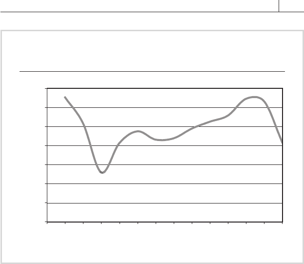
FIGURE 3.1

U.S. Treasury Zero-Coupon Yield Curve in

September 2000

Term to maturity (years)

Log yield

0.73

0.74

0.75

0.76

0.77

0.78

0.79

0.8

012345678910152030

Source: Bloomberg

ship between the spot interest rates of credit-risk–free zero-coupon bonds

and their maturities.

The yield curve is a graph plotting the set of yields

rtt, +

()

through

rtt m, +

()

at time t against m. FIGURES 3.1, 3.2, and 3.3 (above and on

the following page) show the log zero-coupon yield curves, as of Septem-

ber 27, 2000, for, respectively, U.S. Treasury strips, U.K. gilt strips, and

French OAT (Obligations Assimilable du Trésor) strips. The French curve

exhibits the most common shape for yield curves: a gentle upward slope.

The U.K. curve slopes in the opposite direction, a shape termed inverted.

Coupon Bonds

The majority of bonds in the market are coupon bonds. As noted above,

such bonds may be viewed as packages of individual strips. The strips

corresponding to the coupon payments have face values that equal per-

centages of the nominal value of the bond itself, with successively longer

maturity dates; the strip corresponding to the ﬁ nal redemption payment

has the face value and maturity date of the bond.

A bond issued at time i and maturing at time T makes w payments (C

… C

) on w payment dates (t

, … t

w-1

, T ). In the academic literature, these

coupon payments are assumed to be continuous, rather than periodic, so

the stream of coupon payments can be represented formally as a positive

50 Introduction to Bonds

FIGURE 3.3

French OAT Zero-Coupon Yield Curve in

September 2000

Term to maturity (years)

Log yield

0.66

0.68

0.7

0.72

0.74

0.76

0.78

0 3mo 6mo 1 2 3 4 5 6 7 8 9 10 15 20 30

FIGURE 3.2

U.K. Gilt Zero-Coupon Yield Curve in

September 2000

Term to maturity (years)

Log yield

0.58

0.6

0.62

0.64

0.66

0.68

0.7

0.72

0.74

0.76

0.78

0.8

012345678910152030

Source: Bloomberg

Bond Pricing and Spot and Forward Rates 51

function of time:

Ct i t

() < ≤,

. Investors purchasing a bond at time t that

matures at time T pay P(t, T ) and receive the coupon payments as long

as they hold the bond. Note that P(t, T ) is the clean price of the bond, as

deﬁ ned in chapter 1; in practice, unless the bond is purchased for settle-

ment on a coupon date, the investor will pay a dirty price, which includes

the value of the interest that has accrued since the last coupon date.

As discussed in chapter 1, yield to maturity is the interest rate that relates

a bond’s price to its future returns. More precisely, using the notation de-

ﬁ ned above, it is the rate that discounts the bond’s cash ﬂ ow stream C

to its

price P(t, T ). This relationship is expressed formally in equation (3.7).

PtT Ce

ttrtT

()

−−

()

(

)

∑

(3.7)

Expression (3.7) allows the continuously compounded yield to ma-

turity r(t, T ) to be derived. For a zero-coupon, it reduces to (3.5). In the

academic literature,

∑

, which is used in mathematics to calculate sums of

a countable number of objects, is replaced by

∫

, the integral sign, which

is used for an inﬁ nite number of objects. (See Neftci (2000), pages 59–66,

for an introduction to integrals and their use in quantitative ﬁ nance.)

Some texts refer to the graph of coupon-bond yields plotted against ma-

turities as the term structure of interest rates. It is generally accepted, however,

that this phrase should be used for zero-coupon rates only and that the graph

of coupon-bond yields should be referred to instead as the yield curve. Of

course, given the law of one price—which holds that two bonds having the

same cash ﬂ ows should have the same values—the zero-coupon term struc-

ture is related to the yield to maturity curve and can be derived from it.

Bond Price in Continuous Time

This section is an introduction to bond pricing in continuous time. Chap-

ter 4 presents a background on price processes.

Fundamental Concepts

Consider a trading environment in which bond prices evolve in a w-

dimensional process, represented in (3.8).

Xt X t X t X t X t t

()= () () () ()

[]

123

0, , ,....., , (3.8)

where the random variables (variables whose possible values are numerical

outcomes of a random process) X

are state variables, representing the state

of the economy at times t