Carranza E. Geochemical anomaly and mineral prospectivity mapping in GIS

Подождите немного. Документ загружается.

Knowledge-Driven Modeling of Mineral Prospectivity 223

output values of FO. An inference network such as shown in Fig. 7-15 reflects prudence

of the modeler in combining sets of spatial evidence possibly due either to the lack of

‘expert’ knowledge about the inter-play of geological processes represented by

individual sets of spatial evidence or to the average quality of spatial data sets used to

portray the individual sets of spatial evidence.

The output of combining fuzzy sets is also a fuzzy set. For example, the final output

of applying the inference network shown in Fig. 7-15 is shown in Fig. 7-16A. It

represents a fuzzy set of a continuous field of mineral prospectivity values although

there are sharp transitions between low and high values of fuzzy prospectivity values. In

the fuzzy model of epithermal Au prospectivity shown in Fig. 7-16A, there are

apparently many locations with fuzzy prospectivity values equal to zero and there are

relatively less locations with high and very high fuzzy prospectivity values. The former

are due to classes of evidence with fuzzy membership scores of zero, especially the

classes of fuzzy ANOMALY evidence (Table 7-VI), whereas the latter are due to

intersecting classes of evidence with high and very high fuzzy membership scores. The

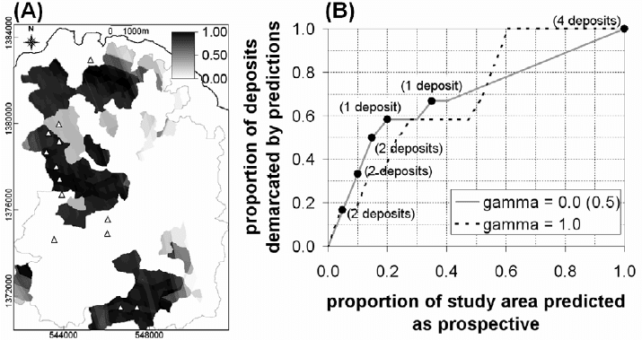
Fig. 7-16. (A) An epithermal Au prospectivity map of Aroroy district (Philippines) obtained via

fuzzy logic modeling based on evidential maps with fuzzy evidential scores shown in Table 7-VI

and on the inference network shown in Fig. 7-15. Triangles are locations of known epithermal Au

deposits; whilst polygon outlined in grey is area of stream sediment sample catchment basins (see

Fig. 4-11). (B) Prediction-rate curves of proportion of deposits demarcated by the predictions

versus proportion of study area predicted as prospective. The prediction-rate curve of the map

obtained by using γ=0.5 is compared with prediction-rate curves of map obtained by using γ=0 and

γ=1 in the final step of the inference network in Fig. 7-15. The prediction-rate curves of the maps

obtained by using γ=0.5 and γ=0 identical, meaning that their prediction-rates are equal. The dots,

which pertain to the prediction-rate curve of the map derived by using γ=0.5, represent classes o

prospectivity values that correspond spatially with a number of cross-validation deposits

(indicated in parentheses).

224 Chapter 7

generic analysis of information (i.e., mineral prospectivity) embedded in a fuzzy set of

values is via defuzzification (Fig. 7-10), so that discrete spatial entities or geo-objects

representing, for example, prospective and non-prospective areas, are recognised or

mapped. Hellendoorn and Thomas (1993) describe a number of criteria for

defuzzification. However, in GIS-based mineral prospectivity mapping, the optimal

method of defuzzifying a fuzzy model of mineral prospectivity is to construct its

prediction-rate curve (see Fig. 7-2) against some cross-validation occurrences of mineral

deposits of the type sought in a study area.

The prediction-rate curve of the fuzzy model of epithermal Au prospectivity in Fig.

7-16A indicates that, if 20% of the case study area is considered prospective, then it

performs equally as well as the multi-class index overlay model of epithermal Au

prospectivity shown in Fig. 7-9. The predictive model in Fig. 7-16A, which is obtained

by using

γ=0.5, performs equally as well as a predictive model obtained by using γ=0 in

the final step of the inference network (Fig. 7-15). Their prediction-rate curves (Fig. 7-

16B) are identical and both of them have better prediction-rates than a predictive model

obtained by using

γ=1 in the final step of the inference network (Fig. 7-16B). These

results imply that the contributions of complementary pieces of spatial evidence provide

better predictions than the contributions of supplementary pieces of spatial evidence.

These results are therefore realistic because epithermal Au mineralisation requires

complementary effects of both structural controls (represented by proximity to NNW-

and NW-trending faults/fractures) and heat source controls (represented by proximity to

intersections of NNW- and NW-trending faults/fractures; see Chapter 6). In addition, the

presence of stream sediment geochemical anomalies is important in indicating locations

of anomalous sources. However, the predictive model obtained by using

γ=1 in the final

step of the inference network is better than the predictive models obtained by using

γ=0

and

γ=0.5 in the final step of the inference network in the sense that the former predicts

all cross-validation deposits if 60% of the case study area is considered prospective

whereas the former predict all cross-validation deposits if 100% of the case study area is

considered prospective (Fig. 7-16B).

The poor performance of the predictive models obtained by using

γ=0 and γ=0.5 in

the final step of the inference network (Fig. 7-15), in terms of correct delineation of all

the cross-validation deposits, is due to classes of evidence with fuzzy membership scores

of zero, especially the classes of fuzzy ANOMALY evidence (Table 7-VI). In Fig. 7-

16A the locations of four cross-validation deposits have output fuzzy prospectivity

values of zero. In order to demonstrate the deleterious effect using a fuzzy membership

score of zero, those classes of fuzzy evidence with fuzzy membership scores of zero in

Table 7-VI are re-assigned the lowest non-zero fuzzy membership scores in the

individual fuzzy sets as shown in Table 7-VII.

The new predictive map (Fig. 7-17A) shows low (rather than zero) fuzzy

prospectivity values at the locations of the four cross-validation deposits not delineated

correctly by the predictive map in Fig. 7-16A. The new results show improvements

mainly for the predictive maps obtained by using

γ=0.5 and γ=0 in the final step of the

inference network, which now delineate correctly all cross-validation deposits if 65%

Knowledge-Driven Modeling of Mineral Prospectivity 225

and 70%, respectively, of the case study area is considered prospective (Fig. 7-17B). The

new results also show that the new predictive map obtained by using

γ=0.5 is slightly

better than the new the predictive map obtained by using

γ=0 (Fig. 7-16B), indicating

that supplementary but subtle pieces of spatial evidence (i.e., those with revised low

fuzzy scores, especially in the fuzzy ANOMALY evidence (Table 7-VI) provide minor

contributions to the improvement of the prediction. Nevertheless, both of the fuzzy

mineral prospectivity models shown in Figs. 7-16 and 7-17 are better than the mineral

prospectivity models derived via Boolean logic modeling (Fig. 7-5), binary index

overlay modeling (Fig. 7-7) and multi-class index overlay modeling (Fig. 7-9). That is

TABLE 7-VII

Examples of fuzzy membership scores assigned to evidential classes in individual evidential maps

portraying the recognition criteria for epithermal Au prospectivity, Aroroy district (Philippines).

Table entries are the same as in Table 7-VI except for the values in bold italics, which are

revisions of initial fuzzy scores of zero. Ranges of values in bold include the threshold value of

spatial data of optimum positive spatial associations with epithermal Au deposits in the study area.

Proximity to NNW

Proximity to FI

Range (km) Mean (km) Fuzzy score Range (km) Mean (km) Fuzzy score

0.00 – 0.08 0.05 0.80 0.00 – 0.39 0.20 0.80

0.08 – 0.15 0.11 0.84 0.39 – 0.58 0.49 0.81

0.15 – 0.23 0.19 0.89 0.58 – 0.80 0.69 0.83

0.23 – 0.32 0.27 0.95

0.80 – 1.09

0.95 0.99

0.32 – 0.41

0.36 1.00 1.09 – 1.40 1.25 0.82

0.41 – 0.52 0.46 0.99 1.40 – 1.80 1.60 0.58

0.52 – 0.71 0.61 0.59 1.80 – 2.32 2.06 0.33

0.71 – 1.06 0.88 0.29 2.32 – 2.92 2.62 0.12

1.06 – 1.73 1.39 0.01 2.92 – 3.62 3.27 0.01

1.73 – 3.55 2.64

0.005

3.62 – 5.92 4.77

0.005

Proximity to NW

ANOMALY

Range (km) Mean (km) Fuzzy score Range Mean Fuzzy score

0.00 – 0.18 0.10 0.80 0.00 – 0.06 0.03

0.01

0.18 – 0.36 0.27 0.84 0.06 – 0.10 0.08

0.03

0.36 – 0.54 0.45 0.89 0.10 – 0.16 0.13

0.06

0.54 – 0.75 0.64 0.94 0.16 – 0.25 0.21 0.12

0.75 – 1.01

0.88 1.00 0.25 – 0.29 0.27 0.88

1.01 – 1.29 1.15 0.99

0.29 – 0.37

0.35 1.00

1.29 – 1.65 1.47 0.93 0.37 – 0.49 0.43 0.96

1.65 – 2.24 1.95 0.75 0.49 – 0.78 0.58 0.90

2.24 – 3.02 2.63 0.03

3.02 – 5.32 4.17

0.01

NNW-trending faults/fractures. Function parameters: α=0.35; β=0.8; γ=1.5.

Intersections of

NNW- and NW-trending faults/fractures. Function parameters: α=1; β=1.9; γ =3.5.

NW-trending

faults/fractures. Function parameters: α=0.9; β=2.3; γ=3.

Integrated PC2 and PC3 scores obtained

from the catchment basin analysis of stream sediment geochemical data (see Chapter 3). Function

parameters: α=0.14; β=0.26; γ=0.34.

226 Chapter 7

because, if 20% of the case study area is considered prospective, then the former models

delineate correctly seven (or about 58%) of the cross-validation deposits (Figs. 7-16B

and 7-17B) whilst the latter models delineate correctly six (or 50%) of the cross-

validation deposits.

The availability of different fuzzy operators and the ability to modify fuzzy inference

networks is an advantage of fuzzy logic modeling compared to binary and multi-class

index overlay modeling. The advantage of fuzzy logic modeling compared Boolean logic

modeling is mainly in the representation of spatial evidence. However, the assignment of

fuzzy evidential scores is as subjective as the assignment of multi-class index scores. No

two experts will arrive at the same fuzzy prospectivity scores to classes of the same set

of spatial evidence. The disadvantage of fuzzy logic modeling compared to multi-class

index overlay modeling is the presumption of equal weights for individual evidential

maps. The common disadvantage of all these modeling techniques is the implicit

representation of uncertainty of spatial evidence. For example, in fuzzy logic modeling

there is no proper and uniform way of assigning fuzzy prospectivity membership scores

Fig. 7-17. (A) An epithermal Au prospectivity map of Aroroy district (Philippines) obtained via

fuzzy logic modeling based on evidential maps with fuzzy evidential scores shown in Table 7-VII

and on the inference network shown in Fig. 7-15. Triangles are locations of known epithermal Au

deposits; whilst polygon outlined in grey is area of stream sediment sample catchment basins (see

Fig. 4-11). (B) Prediction-rate curves of proportion of deposits demarcated by the predictions

versus proportion of study area predicted as prospective. The prediction-rate curve of the map

obtained by using γ=0.5 is compared with prediction-rate curves of map obtained by using γ=0 and

γ=1 in the final step of the inference network in Fig. 7-15. The prediction-rate curves of the maps

obtained by using γ=0.5 and γ=0 mostly overlap each other, meaning that their prediction-rates are

mostly equal. The dots, which pertain to the prediction-rate curve of the map derived by using

γ=0.5, represent classes of prospectivity values that correspond spatially with a number of cross-

validation deposits (indicated in parentheses).

Knowledge-Driven Modeling of Mineral Prospectivity 227

to locations in a study area with missing data. In many case examples in the literature,

locations in a study area without data are assigned either very low fuzzy scores or fuzzy

scores equal to zero. It has been demonstrated above that assignment of fuzzy scores

equal to zero can produce undesirable and unrealistic results. In this volume, locations in

the case study area without stream sediment geochemical data are assigned fuzzy scores

of zero (meaning they are not considered in the analysis), although this has the same net

effect of using fuzzy scores of zero as exemplified in Fig. 7-16A.

The following section explains a different technique of representing and integrating

multi-class evidential maps in order to model mineral prospectivity. This technique –

evidential belief modeling – provides for explicit representation of evidential

uncertainty.

Evidential belief modeling

Dempster’s (1967, 1968) work on the generalisation of Bayesian lower and upper

probabilities provided the basis for the theory of evidential belief. Shafer (1976) then

defined two evidential belief functions (EBFs), belief and plausibility, to represent the

lower and upper probabilities, respectively, that a given body of evidence supports a

particular proposition. In the last three decades or so, the Dempster-Shafer theory of

evidential belief has attracted considerable attention as a promising method of dealing

with some of the basic problems arising in the fusion of data or combination of evidence.

Zadeh (1986) provided a simplification of the Dempster-Shafer theory of evidential

belief and demonstrated the capability of Dempster’s (1968) rule of combination to

integrate distinct probability distributions. Walley (1987) suggested, however, that

Dempster’s (1968) rule of combination is generally neither suitable for combining

evidence from independent observations nor appropriate for combining prior beliefs with

observational evidence. However, applications of the Dempster-Shafer theory of

evidential belief proved its usefulness in combining pieces of evidence from disparate

sources (e.g., Cohen, 1985; Lee et al., 1987; Kim and Swain, 1989). Chung and Fabbri

(1993) described the representation of geoscience information for data integration based

on interpretation of the Dempster-Shafer theory of evidential belief. An et al. (1994b)

demonstrated the management or representation of uncertainty in the integration of

exploration data using EBFs.

The mathematical formalism of the EBFs is complex (Dempster, 1967; Shafer,

1976). The following explanations for the application of EBFs to mineral prospectivity

mapping are simplified and informal. For a piece of spatial evidence that is used in

evaluating a proposition (i.e., mineral prospectivity), four values, each in the range of

[0,1], are assigned based on evaluation of how much it supports the proposition. These

values are belief (hereafter denoted as Bel), disbelief (hereafter denoted as Dis),

uncertainty (hereafter denoted as Unc) and plausibility (hereafter denoted as Pls). The

Bel and Pls represent, respectively, lower and upper degrees of support provided by a

given piece of spatial evidence to the proposition. This means, for example, that with a

given spatial evidence mineral deposit occurrence is either less (Bel) or more (Pls)

likely. Thus, Pls and Bel together represent the vague or uncertain ‘more-or-less’

228 Chapter 7

assessment. The Unc represents ‘ignorance’ or ‘doubt’ that a given piece of spatial

evidence supports the proposition. The value of Unc is the difference between Bel and

Pls. The Dis represents evaluation that a given piece of spatial evidence does not support

the proposition.

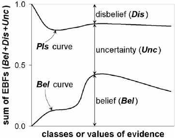
The four EBFs are inter-related (Fig. 7-18). The sum of Bel+Unc+Dis of a piece of

spatial evidence is equal to 1. Likewise, the sum of Pls+Dis of a piece of spatial

evidence is equal to 1. From these two equalities, therefore, Pls = Bel+Unc or Bel = Pls–

Unc. The degree of Unc influences the relation between Bel and Dis. If Unc = 0 (i.e.,

there is complete knowledge about a given piece of spatial evidence), then Bel+Dis = 1

and the relation between Bel and Dis for a given piece of evidence is binary (i.e., Bel =

1–Dis or Dis = 1–Bel), as in the theory of probability. If Unc = 1 (i.e., there is complete

ignorance or doubt about a given piece of spatial evidence), then Bel and Dis for a given

piece of evidence are both equal to zero. That is, if there is complete uncertainty, then

there can be neither belief nor disbelief. Usually, however, Unc is neither equal to zero

nor equal to one. Therefore, in the case that 0<Unc<1, then Bel = 1–Dis–Unc or Dis = 1–

Bel–Unc. This means that, because uncertainty is usually present, the relation between

Bel and Dis for a given piece of evidence is usually not binary. This means further that,

for a piece of evidence used to evaluate a proposition, one should estimate not only Bel

but also Dis and Unc.

In the application of EBFs to knowledge-driven mineral prospectivity mapping, two

of the three EBFs – Bel, Dis and Unc – a

re usually first estimated together in order to

represent not only degree of support (or lack of support) to a proposition by a piece of

spatial evidence but also the degree of uncertainty about this evidence. The Pls is then

simply derived from estimates of any of two EBFs and, as shown below, the Pls is not

used in Dempster’s (1968) rule of combination. Estimating Bel and Dis together is

usually the most difficult, because one tends to think of the binary relation between these

two EBFs and then neglect Unc. Estimating Dis and Unc together is cumbersome,

because of confusion between disbelieving and doubting. So, estimating Bel and Unc

Fig. 7-18. Schematic relationships of evidential belief functions (EBFs). See text for further

explanation.

Knowledge-Driven Modeling of Mineral Prospectivity 229

together is usually the more convenient. In the case that 0<Unc<1, Bel is usually

estimated to be less than or equal to 0.5 but never equal to 0.0. Meanwhile, the value of

Unc is estimated such that (1) the sum Bel+Unc (i.e., Pls) is more than 0.5 but never

equal to 1.0, (2) the estimates of Bel and Unc vary inversely, (3) the derived values of

Dis vary inversely with the estimates of Bel and co-vary with the estimates of Unc.

These three conditions are important in order to represent the following realistic relations

of the EBFs in the case that 0<Unc<1. Firstly, the higher the uncertainty, the lower the

belief or vice versa. Secondly, the higher the belief, the lower the disbelief or vice versa.

Thus, in the usual case that 0<Unc<1, the estimates of Bel are kept asymptotic to 0.0,

whereas the sum Bel+Unc is kept asymptotic to 1.0. The above-stated conditions for

knowledge-driven estimation of Unc together with Bel do not apply when there is either

complete ignorance or doubt (i.e., Unc=1) or complete knowledge (i.e., Unc=0) about a

piece of spatial evidence in relation to a proposition. An example situation of Unc=1 in

mineral prospectivity mapping is when spatial data are missing. There is no situation of

Unc=0 in mineral prospectivity mapping because if Unc were equal to zero there would

be no need for mineral prospectivity mapping.

Once Bel and Unc have been estimated, for the case of 0<Unc<1, the remaining two

EBFs (Dis, Pls) can be easily estimated based on the inter-relations of the EBFs

explained above and illustrated in Fig. 7-18. Examples of knowledge-driven estimations

of EBFs for mineral prospectivity mapping can be found in Moon (1990, 1993), Chung

and Moon (1991), Moon et al. (1991), An (1992), An et al. (1992, 1994a, 1994b), Chung

and Fabbri (1993), Wright and Bonham-Carter (1996), Likkason et al. (1997), Carranza

(2002), Tangestani and Moore (2002) and Rogge et al. (2006). In practise, knowledge-

driven estimates of EBFs are assigned and stored in attribute tables associated with

individual maps of spatial data to be used as evidence of mineral prospectivity (see Fig.

7-1). For the present mineral prospectivity case study, Table 7-VIII shows examples of

Bel, Unc and Dis estimated for evidential classes of the same sets of evidential maps

used in the multi-class index and fuzzy logic modeling (see Tables 7-V to 7-VII). The

estimates of Bel, like the estimates of the multi-class index scores and the fuzzy

membership scores (see Tables 7-V and 7-VI, respectively), are according to the

knowledge of spatial associations between the epithermal Au deposit occurrences and

the individual sets of spatial data to be used as evidence of epithermal Au prospectivity

in the case study area. In accordance with the three conditions given above for

estimating Bel and Unc together, Table 7-VIII sh

ows that the estima

tes of Bel vary

inversely with estimates of Unc and the derived values of Dis vary inversely with the

estimates of Bel and co-vary with the estimates of Unc. The locations without stream

sediment geochemical data are assigned Bel=0 and Unc=1 and, thus, Dis=0.

For each spatial evidence map X

(i=1,2,…,n), three attribute maps representing EBFs

Bel

, Dis

and Unc

are then created. The maps of EBFs associated with spatial evidence

map X

can be combined with the maps of EBFs associated with spatial evidence map X

according to Dempster’s (1968) rule of combination, which can be implemented by

using either an AND or an OR operation (An et al., 1994a).

230 Chapter 7

The formulae for combining EBFs of two spatial evidence maps (X

, X

) according to

an AND operation are defined as (An et al., 1994a):

BelBel

Bel

, (7.14)

DisDis

Dis

, and (7.15)

TABLE 7-VIII

Examples of values of EBFs assigned to evidential classes in individual evidential maps

ortraying the recognition criteria for epithermal Au prospectivity, Aroroy district (Philippines).

Values of Bel and Unc are first estimated together and then Dis is derived as 1–Bel–Unc (see text

for further explanation). Ranges of values in bold include the threshold value of spatial data of

optimum positive spatial associations with epithermal Au deposits in the case study area.

Proximity to NNW

Proximity to FI

Range (km) Bel Unc Dis Range (km) Bel Unc Dis

0.00 – 0.08 0.30 0.44 0.26 0.00 – 0.39 0.30 0.44 0.26

0.08 – 0.15 0.35 0.43 0.22 0.39 – 0.58 0.40 0.42 0.18

0.15 – 0.23 0.40 0.42 0.18 0.58 – 0.80 0.45 0.41 0.14

0.23 – 0.32 0.45 0.41 0.14

0.80 – 1.09

0.50 0.40 0.10

0.32 – 0.41

0.50 0.40 0.10 1.09 – 1.40 0.40 0.42 0.18

0.41 – 0.52 0.40 0.42 0.18 1.40 – 1.80 0.20 0.46 0.34

0.52 – 0.71 0.30 0.44 0.26 1.80 – 2.32 0.10 0.47 0.43

0.71 – 1.06 0.20 0.46 0.34 2.32 – 2.92 0.05 0.48 0.47

1.06 – 1.73 0.10 0.48 0.42 2.92 – 3.62 0.03 0.49 0.48

1.73 – 3.55 0.05 0.50 0.45 3.62 – 5.92 0.01 0.50 0.49

Proximity to NW

ANOMALY

Range (km) Bel Unc Dis Range Bel Unc Dis

0.00 – 0.18 0.30 0.44 0.26 No data 0.00 1.00 0.00

0.18 – 0.36 0.35 0.43 0.22 0.00 – 0.06 0.05 0.50 0.45

0.36 – 0.54 0.40 0.42 0.18 0.06 – 0.10 0.10 0.48 0.42

0.54 – 0.75 0.45 0.41 0.14 0.10 – 0.16 0.15 0.46 0.39

0.75 – 1.01

0.50 0.40 0.10 0.16 – 0.25 0.25 0.44 0.31

1.01 – 1.29 0.40 0.42 0.18 0.25 – 0.29 0.35 0.43 0.22

1.29 – 1.65 0.30 0.47 0.23

0.29 – 0.37

0.50 0.40 0.10

1.65 – 2.24 0.20 0.48 0.32 0.37 – 0.49 0.45 0.41 0.14

2.24 – 3.02 0.10 0.49 0.41 0.49 – 0.78 0.40 0.42 0.18

3.02 – 5.32 0.05 0.50 0.45

NNW-trending faults/fractures.

Intersections of NNW- and NW-trending faults/fractures.

NW-

trending faults/fractures.

Integrated PC2 and PC3 scores obtained from the catchment basin

analysis of stream sediment geochemical data (see Chapter 3).

Knowledge-Driven Modeling of Mineral Prospectivity 231

++++

1221122121

XXXXXXXXXX

UncDisUncDisUncBelUncBelUncUnc

Unc

(7.16)

where

2121

XXXX

BelDisDisBel −−=β

, which is a normalising factor ensuring that

1=++ DisUncBel . Equations (7.14) and (7.15) are multiplicative, so that the application

of an AND operation results in a map of integrated Bel and integrated Dis, respectively,

in which the output values represent support and lack of disbelief, respectively, for the

proposition being evaluated if pieces of spatial evidence in two input maps coincide (or

intersect). In contrast, equation (7.16) is both commutative and associative, so that the

application of an AND operation results in a map of integrated Unc in which the output

values are controlled by pieces of spatial evidence with large uncertainty in either of the

two input maps. Therefore, an AND operation is suitable in combining two pieces of

complementary spatial evidence (say, X

and X

) in order to support the proposition of

mineral prospectivity. In mineral exploration, proximity to faults/fractures and stream

sediment geochemical anomalies can represent two sets of complementary spatial

evidence of mineral deposit occurrence, because several types of mineral deposits,

including epithermal Au, are localised along faults/fractures and, if exposed at the

surface, can release metals into the drainage systems and cause anomalous

concentrations of metals in stream sediments. (After application of equations (7.14)–

(7.16),

Pls is derived according to the relationships of the EBFs explained above.)

The formulae for combining EBFs of two spatial evidence maps (X

, X

) according

to an OR operation are defined as (An et al., 1994a):

122121

XXXXXX

UncBelUncBelBelBel

Bel

(7.17)

122121

XXXXXX

UncDisUncDisDisDis

Dis

(7.18)

UncUnc

Unc

(7.19)

where

β is the same as in equations (7.14)–(7.16). Equations (7.17) and (7.18) are both

commutative and associative, so that the application of OR operation results in a map of

integrated

Bel and integrated Dis, respectively, in which the output values are controlled

by pieces of spatial evidence with large belief or large disbelief in either of the two input

maps. In contrast, equation (7.19) is multiplicative, so that the application of an OR

operation results in a map of integrated

Unc in which the output values is controlled by

pieces of spatial evidence with low uncertainty in either of the two input maps.

Therefore, an OR operation is suitable in combining two pieces of supplementary (as

232 Chapter 7

opposed to complementary) spatial evidence (say, X

and X

) in order to support the

proposition of mineral prospectivity. In mineral exploration, proximity to faults/fractures

and stream sediment geochemical anomalies can represent two sets of supplementary

spatial evidence of the presence of mineral deposits, because not all locations proximal

to faults/fractures contain mineral deposits and because not all stream sediment

geochemical anomalies necessarily mean the presence of mineral deposits. (After

application of equations (7.17)–(7.19),

Pls is derived according to the

relationships of the EBFs explained above.)

According to Dempster’s rule of combination, only EBFs of two spatial evidence

maps can be combined each time. The EBFs of maps

,…,X

are combined with already

integrated EBFs one after another by re-applying either equations (7.14)–(7.16) or

equations (7.17)–(7.19) as deemed appropriate. The final integrated values of

Bel are

considered indices of mineral prospectivity. Furthermore, because equation (7.14) is

multiplicative, whilst equation (7.17) is associative and commutative, the output

integrated values of

Bel derived via the former are always less than the corresponding

output integrated values of

Bel derived via the latter. This means that integrated values

of EBFs should not be interpreted in absolute terms but in relative terms (i.e., ordinal

scale) only and, therefore, in mineral prospectivity modeling integrated values of

Bel

represent relative degrees of likelihood for mineral deposit occurrence.

As in Boolean logic modeling and in fuzzy logic modeling of mineral prospectivity,

an inference network is useful in combining logically EBFs of spatial evidence of

mineral prospectivity. The inference network used in the Boolean logic modeling (Fig.

7-4), which is more-or-less similar to the inference network used in the fuzzy logic

modeling (Fig. 7-15), is applied to logically integrate the EBFs of the spatial evidence

maps of epithermal Au prospectivity in the case study area. The geological reasoning

behind the integration of the EBFs of the spatial evidence maps of epithermal Au

prospectivity in the case study area is, thus, the same as in the earlier application of

Boolean logic modeling and similar to the earlier application of the fuzzy logic

modeling. The map of integrated

Bel (Fig. 7-19A) shows a pattern of prospective areas

that is more similar to the pattern of prospective areas delineated via multi-class index

overlay modeling (Fig. 7-9A) and via fuzzy logic modeling (Figs. 7-16A and 7-17A)

than the pattern of prospective areas delineated via Boolean logic modeling (Fig. 7-5A)

and via binary index overlay modeling (Fig. 7-7A). However, unlike the earlier mineral

prospectivity maps, a prediction-rate curve (Fig. 7-19B) can be constructed for the

mineral prospectivity map in Fig. 7-19A with respect to the whole case study area

because, for the locations without stream sediment geochemical evidence, there are input

EBFs (i.e.,

Bel=0, Unc=1 and Dis=0) and thus output EBFs. Nevertheless, for proper

comparison of predictive performance with the earlier mineral prospectivity maps, a

prediction-rate curve with respect only to locations with stream sediment geochemical

evidence is also constructed (Fig. 7-19C). Using this curve, if 20% of the case study area

is considered prospective, the map of integrated

Bel delineates correctly seven (or about

58%) of the cross-validation deposits (Fig. 7-19C). This predictive performance of the

evidential belief model (Fig. 7-19A) is the same as that of the fuzzy logic model (Fig. 7-