Carranza E. Geochemical anomaly and mineral prospectivity mapping in GIS

Подождите немного. Документ загружается.

Knowledge-Driven Modeling of Mineral Prospectivity 193

values, it is instructive to start as much as possible with several narrow equal-area or

equal-percentile classes and then to combine them, as necessary, into wider equal-area or

equal-percentile classes in order to achieve a monotonically descending histogram.

Secondly, the mineral prospectivity map is crossed with or intersected by the map of

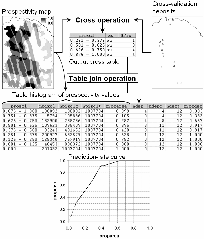
Fig. 7-2. Schematic GIS-based procedures for cross-validating the performance of a mineral

prospectivity map. The objective is to create a prediction-rate curve, which allows mapping o

optimal prospective areas. See text for further explanations, especially the variables in the tables.

194 Chapter 7

cross-validation deposits. The output cross table contains information about number

(

Npix) of cross-validation known deposits (au) contained in a class of prospectivity

values (

proscl). Values in the Npix column of the cross table are joined to a column

(

ndep) in the table histogram of prospectivity values for subsequent calculation of the

cumulative number of deposits (

ndepc), total number of deposits (ndept) and the

proportion of deposits per prospectivity class (

propdep). Values in the column

propdep are then derived by dividing values in the column ndepc with corresponding

values in the column

ndept. Finally, a prediction-rate graph of propdep values versus

proparea values is created.

The prediction-rate curve allows estimation of likelihood of mineral deposit

discovery according to the prospectivity map. Any point along the prediction-rate curve

represents a prediction of prospective zones with a corresponding number of delineated

deposits and number of unit cells or pixels, so the ratio of the former to the latter is

related to the degree of likelihood of mineral deposit occurrence (or discovery) in the

delineated prospective zones. This means that, the higher the value of

propdep÷proparea of predicted prospective zones (Fig. 7-2), the better is the

prediction. It is, therefore, ideal to obtain a mineral prospectivity map with a steep

prediction-rate curve. However, the performance of a mineral prospectivity map is

influenced by (a) the quality of the input spatial data and (b) the way by which evidential

maps are created (i.e., the number of evidential classes per evidential map) and

integrated and, thus, by the modeling technique applied to create a mineral prospectivity

map. We now turn to the concepts of individual modeling techniques that are applicable

to knowledge-driven mapping of mineral prospectivity.

MODELING WITH BINARY EVIDENTIAL MAPS

In this type of modeling, evidential maps representing prospectivity recognition

criteria contain only two classes of evidential scores – maximum evidential score and

minimum evidential score (Figs. 7-1 and 7-3). Maximum evidential score is assigned to

spatial data representing presence of indicative geological features and having optimum

positive spatial association with mineral deposits of the type sought. Minimum evidential

score is assigned to spatial data representing absence of indicative geological features

and lacking positive spatial association with mineral deposits of the type sought. There

are no intermediate evidential scores in modeling with binary evidential maps. This

knowledge-based representation is usually inconsistent with real situations. For example,

whilst certain mineral deposits may actually be associated with certain faults, the

locations of some mineral deposit occurrences indicated in maps are usually, if not

always, the surface projections of their positions in the subsurface 3D-space, whereas the

locations of faults indicated in maps are more-or-less their ‘true’ surface locations (Fig.

7-3). Thus, for locations within the range of distances to such faults where positive

spatial association with mineral deposits is optimal, the evidential scores should not be

uniformly equal to the maximum evidential score. Likewise, for locations beyond the

distance to faults with threshold optimum positive spatial association to the mineral

Knowledge-Driven Modeling of Mineral Prospectivity 195

deposits, the evidential scores should not be uniformly equal to the minimum evidential

score. The same line of reasoning can be accorded to the binary representation of

evidence for presence of surficial geochemical anomalies, which may be significant

albeit allochthonous (i.e., located not directly over the mineralised source) (Fig. 7-3).

Note also that the graph of binary evidential scores versus data of spatial evidence is

inconsistent with the shapes of the D curves (Figs. 6-9 to 6-12) in the analyses of spatial

associations between epithermal Au deposit occurrences and individual sets of spatial

evidential data in the case study area. Nevertheless, binary representation of evidence of

mineral prospectivity is suitable in cases when the level of knowledge applied is lacking

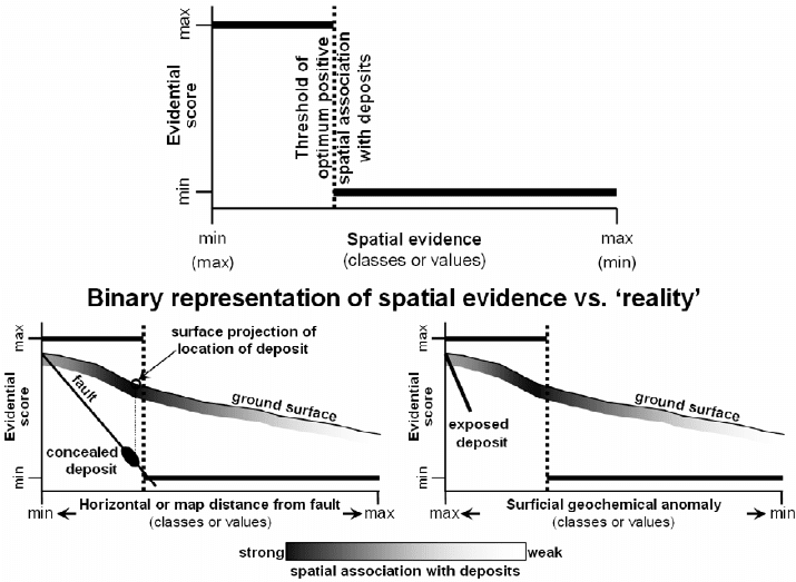
Fig. 7-3. Knowledge-

ased binary representation of spatial evidence of mineral prospectivity.

Knowledge of spatial association between mineral deposits of the type sought and spatial data o

indicative geological features is applied to assign binary evidential scores (upper part of the

figure). If values or classes of values of spatial data have optimum positive spatial association with

mineral deposits of the type sought, they are given a maximum evidential score of mineral

rospectivity; otherwise, they are given a minimum evidential score of mineral prospectivity.

These scores are discontinuous, meaning there are no intermediate evidential scores of mineral

rospectivity. Binary representation of spatial evidence is inconsistent with real situations o

spatial associations between mineral deposits and indicative geological features. For visual

comparison, the graph in the upper part of the figure is overlaid on schematic cross-sections o

ground conditions (lower part of the figure), but the y-axis of the graph does represent vertical

scale of the cross-sections. See text for further explanation.

196 Chapter 7

or incomplete and/or when the accuracy or resolution of available spatial data is poor.

We now turn to the individual techniques for knowledge-based binary representation and

integration of spatial evidence that can be used in order to derive a mineral prospectivity

map.

Boolean logic modeling

Ample explanations of Boolean logic applications to geological studies can be found

in Varnes (1974) and/or Robinove (1989), whilst examples of Boolean logic applications

to mineral prospectivity mapping can be found in Bonham-Carter (1994), Thiart and De

Wit (2000) and Harris et al. (2001b).

In the application of Boolean logic to mineral prospectivity mapping, attributes or

classes of attributes of spatial data that meet the condition of a prospectivity recognition

criterion are labelled TRUE (or given a class score of 1); otherwise, they are labelled

FALSE (or given a class score of 0). Thus, a Boolean evidential map contains only class

scores of 0 and 1. Every Boolean evidential map has equal weight in providing support

to the proposition under examination; that is because in the concept of Boolean logic

there is no such thing as, say, “2×truth”. Thus, the class scores of 0 and 1 in a Boolean

evidential map are only symbolic and non-numeric.

Boolean evidential maps are combined logically according to a network of steps,

which reflect inferences about the inter-relationships of processes that control the

occurrence of a geo-object (e.g., mineral deposits) and spatial features that indicate the

presence of that geo-object. The logical steps of combining Boolean evidential maps are

illustrated in a so-called inference network. Every step, whereby at least two evidential

maps are combined, represents a hypothesis of inter-relationship between two sets of

processes that control the occurrence of a geo-object (e.g., mineral deposits) and/or

spatial features that indicate the presence of the geo-object. A Boolean inference

network makes use of set operators such as AND and OR. The AND (or intersection)

operator is used if it is considered that at least two sets of spatial evidence must be

present together in order to provide support to the proposition under examination. The

OR (or union) operator is used if it is considered that either one of at least two sets of

spatial evidence is sufficient to provide support to the proposition under examination.

Boolean logic modeling is not exclusive to using only the AND and OR operators,

although the other Boolean operators (e.g., NOT, XOR, etc.) are not commonly applied

in GIS-based knowledge-driven mineral prospectivity mapping. The output of

combining evidential maps via Boolean logic modeling is a map with two classes, one

class represent locations where all or most of the prospectivity recognition criteria are

satisfied, whilst the other class represents locations where none of the prospectivity

recognition criteria is satisfied.

For the case study area, Boolean evidential maps are prepared from the individual

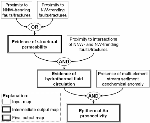
spatial data sets according to the prospectivity recognition criteria given above. Fig. 7-4

shows the inference network for combining the evidential maps based on the given

spatial data sets. The Boolean evidential maps of proximity to NNW-trending

faults/fractures and proximity to NW-trending faults/fractures are first combined by

Knowledge-Driven Modeling of Mineral Prospectivity 197

using the OR operator in order to represent a hypothesis of structural permeability. The

OR operator is used because it is plausible that at certain locations either set of

faults/fractures can be a predominant control on structural permeability required for the

plumbing system in epithermal mineralisation. The intermediate Boolean evidential map

of structural permeability is then combined with the Boolean evidential map of

proximity to intersections of NNW- and NW-trending faults by using the AND operator.

The latter map is considered a proxy evidence for heat source control on hydrothermal

fluid circulation (see Chapter 6). Thus, the AND operator is used because heat source

and structural permeability controls are both essential controls on hydrothermal fluid

circulation. Finally, the evidential map representing hydrothermal fluid circulation is

combined with the Boolean evidential map of multi-element stream sediment

geochemical anomalies by using the AND operator. The AND operator is used because

the presence of indications of hydrothermal fluid circulation (e.g., hydrothermal altered

rocks) does not necessarily mean the presence of mineralisation and the presence of

stream sediment anomalies does not necessarily indicate the presence of mineral deposit

occurrences, so that the presence of both types of evidence would be more indicative of

the presence of a mineral deposit occurrence in the vicinity.

The final Boolean output map of epithermal Au prospectivity (Fig. 7-5A) shows

strong influence of the multi-element geochemical anomaly evidence, which is a

consequence of using the AND operator in the final step of the inference network (Fig.

7-4). The pattern of prospective areas shown in Fig. 7-5A is similar to the pattern of

highly significant anomalies shown in Fig. 5-14; the latter map is derived as a product

Fig. 7-4. An inference network for combining input Boolean evidential maps for modeling o

epithermal Au prospectivity in the Aroroy district (Philippines).

198 Chapter 7

(i.e., by multiplication) of the same multi-element geochemical anomaly evidence and

fault/fracture density. Thus, the Boolean AND operator has a multiplicative net effect. In

contrast, the Boolean OR operator has an additive net effect, which is unsuitable is many

cases, such as in combining the Boolean evidential map of hydrothermal fluid circulation

and the Boolean evidential map of multi-element stream sediment geochemical

anomalies. Doing so results in a large prospective area with a low prediction-rate. Note,

however, that the application of the Boolean AND operator returns an output value only

for locations with available data in both input evidential maps. Thus, for the case study

area, locations with missing stream sediment geochemical data do not take on predicted

prospectivity values by application of Boolean logic modeling (Fig. 7-5A).

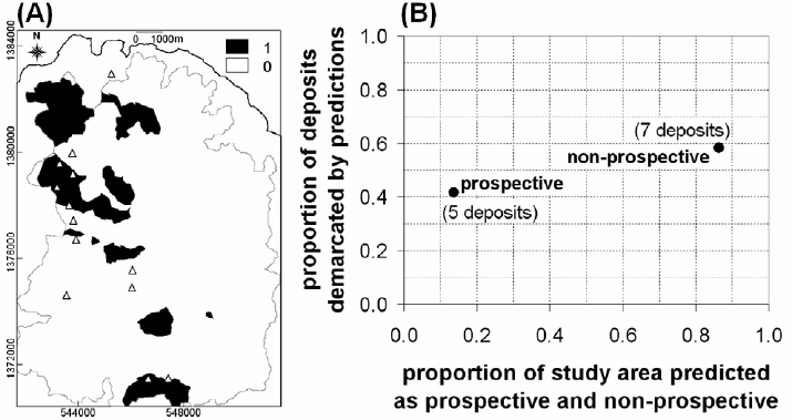
Cross-validation of a Boolean mineral prospectivity map results in a plot with only

two points, one representing completely prospective areas and the other representing

completely non-prospective areas, which should not be connected to form a prediction-

rate curve (Fig. 7-5B). In the Boolean epithermal Au prospectivity map of the case study

area, prospective zones contain about 42% of the cross-validation deposits and occupy

about 14% of the study area, whereas non-prospective zones contain about 58% of the

cross-validation deposits and occupy about 86% of the study area. Estimates of ratios of

the proportion of cross-validation deposits delineated to the corresponding proportion of

the prospective or non-prospective areas suggest that there is at least four times higher

likelihood of epithermal Au deposit occurrence in the predicted prospective areas than in

Fig. 7-5. (A) An epithermal Au prospectivity map obtained by application of an inference network

(Fig. 7-4) for Boolean logic modeling, Aroroy district (Philippines). 1 = prospective zones; 0 =

non-prospective zones. Triangles are locations of known epithermal Au deposits; whilst polygon

outlined in grey is area of stream sediment sample catchment basins (see Fig. 4-11). (B) Plots o

roportion of deposits demarcated by the predictions versus proportion of study area predicted as

prospective and non-prospective. The numbers of cross-validation deposits delineated in

prospective and non-prospective zones are indicated in parentheses.

Knowledge-Driven Modeling of Mineral Prospectivity 199

the predicted non-prospective areas. The significance of this performance of the Boolean

epithermal Au prospectivity map of the case study area can be appreciated by comparing

it with the performances of other mineral prospectivity maps derived via the other

modeling techniques.

Binary index overlay modeling

In binary index overlay modeling, attributes or classes of attributes of spatial data

that satisfy a prospectivity recognition criterion are assigned a class score of 1;

otherwise, they are assigned a class score of 0. Therefore, a binary index map is similar

to a Boolean map, except that the values in the former are both symbolic and numeric.

So, a binary index map is amenable to arithmetic operations. Consequently, each binary

evidential map B

(i=1,2,…,n) can be given (i.e., multiplied with) a numerical weight W

based on ‘expert’ judgment of the relative importance of a set of indicative geological

features represented by an evidential map with respect to the proposition under

examination.

The weighted binary evidential maps are combined using the following equation,

which calculates an average score, S, for each location (cf. Bonham-Carter, 1994):

(7.1)

where W

is weight of each B

(i=1,2,…,n) binary evidential map. In the output map S,

each location or pixel takes on values ranging from 0 (i.e., completely non-prospective)

to 1 (i.e., completely prospective). So, although the input maps only have two classes,

the output map can have intermediate prospectivity values, which is more intuitive than

the output in Boolean logic modeling. Examples of mapping mineral prospectivity via

binary index overlay modeling can be found in Bonham-Carter (1994), Carranza et al.

(1999), Thiart and De Wit (2000) and Carranza (2002).

Assignment of meaningful weights to individual evidential maps is a highly

subjective exercise and it may involve a trial-and-error procedure, even in the case when

‘real expert’ knowledge is available particularly from different experts. The difficulty

lies in deciding objectively and simultaneously how much more important or how much

less important is one evidential map compared to every other evidential map. This

difficulty may be overcome by making pairwise comparisons among the evidential maps

in the context of a decision making process known as the analytical hierarchy process

(AHP). The concept of the AHP was developed by Saaty (1977, 1980, 1994) for

pairwise analysis of priorities in multi-criteria decision making. It aims to derive a

hierarchy of criteria based on their pairwise relative importance with respect to the

objective of a decision making process (e.g., evaluation of the mineral prospectivity

proposition). Most GIS-based applications of the AHP concern land-use allocations (e.g.,

200 Chapter 7

Eastman et al., 1995). De Araújo and Macedo (2002), Moreira et al. (2003) and

Hosseinali and Alesheikh (2008) provide case applications of the AHP to derive criteria

or evidential map weights for mineral prospectivity mapping. The application of the

AHP is useful not only for binary index overlay modeling but also for multi-class index

overlay modeling (see further below) and fuzzy logic modeling.

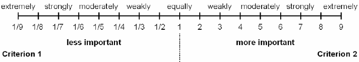
The method of deriving criteria weights via the AHP involves pairwise comparisons

of criteria according to their relative importance with respect to a proposition. The

method adopts a 9-point continuous pairwise rating scale for judging whether Criterion X

is less important or more important than Criterion Y (Fig. 7-6). The relative importance

rating is read from the either the left or right extremity of the scale, depending (a) on

which extremity each of two criteria is positioned and (b) on which criterion is compared

to the other. In addition, the importance rating of one criterion is always the inverse of

the importance rating of the other criterion. For example, if Criterion 1 and Criterion 2

are positioned at the left extremity and right extremity, respectively, and if Criterion 1 is

‘weakly’ less important compared to Criterion 2, then the relative importance rating of

Criterion 1 compared to Criterion 2 is 1/3. It follows that the relative importance rating

of Criterion 2 compared to Criterion 1 is 3. Reversing the positions of Criterion 1 and

Criterion 2 does not change their relative importance ratings. Thus, if Criterion 1 and

Criterion 2 are now positioned at the right extremity and left extremity, respectively, and

if Criterion 2 is ‘weakly’ more important compared Criterion 1, then the relative

importance rating of Criterion 2 compared to Criterion 1 is 3. It follows that the relative

importance rating of Criterion 1 compared to Criterion 2 is 1/3. The pairwise relative

importance ratings of all possible pairs of criteria are then entered into a pairwise

comparison matrix.

For the epithermal Au prospectivity recognition criteria in our case study area, the

pairwise comparisons of relative importance of each criterion (Table 7-I) are based on

the results of the spatial analyses in Chapter 6. Proximity to NNW-trending

faults/fractures is considered to be between moderately and strongly more important than

proximity to intersections of NNW- and NW-trending faults/fractures; thus, a rating of 6

is given to the former. This is because, in the case study area, the NNW-trending

faults/fractures seem to have more influence in the formation of dilational jogs (Fig. 6-

16), which are known to be favourable sites for mineralisation. Proximity to NNW-

trending faults/fractures is considered moderately more important than proximity to NW-

trending faults/fractures; thus a rating of 5 is given to the former. This is because, in the

Fig. 7-6. Continuous rating scale for pairwise comparison of relative importance of one criterion

versus another criterion with respect to a proposition (adapted from Saaty, 1977).

Knowledge-Driven Modeling of Mineral Prospectivity 201

case study area, the known epithermal Au deposit occurrences are more strongly

spatially associated with NNW-trending faults/fractures than with NW-trending

faults/fractures. Proximity to intersections of NNW- and NW-trending faults/fractures is

considered moderately more important that proximity to NW-trending faults/fractures;

thus a rating of 5 is given to the former. This is because dilational jogs in the case study

area, which generally coincide with intersections of NNW- and NW-trending

faults/fractures, seem to be more associated with NNW-trending faults/fractures rather

than with NW-trending faults/fractures. The catchment basin anomalies of stream

sediment geochemical data are considered to be between moderately more important

than and equally important as proximity to individual sets of structures; thus, a rating of

2 is given to the former.

When a matrix of pairwise importance ratings for all possible pairs of criteria is

obtained, the next step is to estimate the eigenvectors of the matrix (cf. Boroushaki and

Malczewski, 2008). Good approximations of the eigenvectors of the pairwise

comparison matrix can be achieved by normalising the pairwise ratings down each

column and then by calculating criterion weight as the average of the normalised

pairwise ratings across each row (Tables 7-I and 7-II). For example, in column NNW in

Table 7-I, the sum of the pairwise ratings is 3.37. By dividing each pairwise rating in

that column by 3.37, we obtain the normalised pairwise ratings for the same column

(Table 7-II). This procedure is repeated for all the columns in the matrix. Then, the

fractional weight of each criterion is obtained by averaging the normalised pairwise

ratings across a row (Table 7-II). The sum of the fractional criteria weights is

approximately equal to 1 (Table 7-II), reflecting approximately 100% of the explained

variance of the values in the matrix.

The fractional criteria weights obtained can then be used in equation (7.1).

Alternatively, instead of using the fractional criteria weights, they can be converted into

TABLE 7-I

Example of a matrix of pairwise ratings (see Fig. 7-6) of relative importance of recognition criteria

for epithermal Au prospectivity in Aroroy district (Philippines). Values in bold are used for

demonstration in Table 7-II, whilst values in bold italics are used for demonstrations in Tables 7-II

and 7-III.

Criteria

NNW FI NW ANOMALY

NNW

1 5 6 1/2

1/5

1 5 1/2

1/6

1/5 1 1/2

ANOMALY

2 2 1

Sum

3.37 8.2 14 2.5

Criteria: NNW = proximity to NNW-trending faults/fractures; NW = proximity to NW-trending

faults/fractures; FI = proximity to intersections of NNW- and NW-trending faults/fractures:

ANOMALY = integrated PC2 and PC3 scores obtained from the catchment basin analysis o

stream sediment geochemical data (see Chapter 3).

Sum of ratings down columns.

202 Chapter 7

integers or whole numbers by dividing each of the fractional criteria weights by the

smallest fractional criterion weight (Table 7-II). The integer criteria weights are more

intuitive than the fractional criteria weights. Before using either the fractional or integer

criteria weights obtained via the AHP, it is important to determine if the pairwise rating

matrix and thus the derived weights are consistent, which also reflects the consistency of

the ‘expert’ judgment applied in assigning the pairwise relative importance ratings.

A matrix is consistent if every value across each row is a multiple of every other

value in the other rows. This is not the case of the matrix in Table 7-I, meaning that there

is some degree of inconsistency among the pairwise ratings in the matrix. In addition,

pairwise ratings are consistent if they are transitive. This means, for example from Table

7-I, that because the weight for NNW is 5× the weight for FI (or, NNW=5×FI) and the

weight for NNW is 6× the weight of NW (or, NNW=6×NW), then the weight for FI

should be 6/5× but not 5× the weight for NW (or, FI=6/5×NW≠5×NW). However, one

may argue that transitive pairwise ratings are not intuitively representative of knowledge

or judgment of inter-play of geological processes involved in a complex phenomenon

such as mineralisation. Nevertheless, when applying the AHP, it is imperative to

quantify and determine whether inconsistencies in a pairwise comparison matrix are

within acceptable limits.

A n×n matrix (n = number of factors or criteria), such as a pairwise comparison

matrix, is consistent if it has one eigenvalue with a value equal to n; otherwise it has at

most n eigenvalues with values varying around n (Saaty, 1977). The inconsistency of a

matrix is then related to how much the mean of eigenvalues (λ) of such matrix deviates

from n. According to Saaty (1977), the eigenvalues of the pairwise comparison matrix

may be estimated from the pairwise importance ratings (Table 7-I) and the estimates of

the eigenvectors or criteria weights (Table 7-II). Approximations of the eigenvalues can

be referred to as the consistency vectors (CV) of the individual criteria (Table 7-III). The

TABLE 7-II

Example of calculation of weights of recognition criteria for epithermal Au prospectivity in

Aroroy district (Philippines). Values in bold and bold italics are taken from Table 7-I. Underlined

values are used for demonstration in Table 7-III.

Criteria

NNW FI NW ANOMALY

Fractional

weight

)

Integer

weight

)

NNW

1 ÷ 3.37

= 0.30

5 ÷ 8.2

= 0.61

6 ÷ 14

= 0.43

1/2 ÷ 2.5

= 0.2

0.39

1/5 ÷ 3.37

= 0.06

0.36 0.12 0.2 0.19 2

1/6 ÷ 3.37

= 0.05

0.07 0.02 0.2 0.09

ANOMALY

2 ÷ 3.37

= 0.59

0.14 0.24 0.4 0.34

See footnotes to Table 7-I.

Example: fractional weight

NNW

= (0.30+0.61+0.43+0.2) ÷ 4 = 0.39.

= W

÷ [min(W

)].