Carlip S. Quantum Gravity in 2+1 Dimensions

Подождите немного. Документ загружается.

76 4

Geometric

structures and Chern-Simons theory

By (3.82), the symplectic structure is now

dpi

5TI + dp

AST

= S (Srf

5r^ - <5rf

<5r

j),

(4.39)

so (r^rj) and (rf,r^~) are the two conjugate pairs. This is a particular

case of a more general phenomenon: when A < 0, the two copies of

SL(2,R) that define the geometric structure have independent symplectic

structures. Note that the Hamiltonian in (4.38) generates translations in

T; the corresponding generator of translations in 1 is

2i , _ , + _* 2 It

( 2 2

\i/2

= -*;Hred = esc - (r

- r\r

) = - esc -

+ p

) .

A similar quotient construction exists for the (2+l)-dimensional black

hole [71]. Indeed, the identifications (3.61) of chapter 3 are an isometry

of anti-de Sitter space, and can be represented by the

SL(2,

R) x

SL(2,

holonomy (R

,R~) with

. e"(r

-r-W 0 \

~ ' 0

-Mr+-r-)/f I '

0 \

where r+ are the inner and outer horizons (3.46). This quotient construc-

tion will be discussed further in chapter 12.

For A > 0, the situation is rather different. The relevant simply

connected model space is now de Sitter space, and the holonomies lie in

the isometry group

(3,1).

In this case, it is not true that the holonomies

uniquely determine the geometric structure; as discussed in the preceding

section, a given holonomy typically corresponds to an infinite number of

distinct spacetimes.

For the torus topology, for example, a pair of commuting holonomies

may be put in the form

(4.42)

These act on the coordinates (T,X,Y,Z) of equation (4.22) by ordinary

matrix multiplication. The coordinate transformation analogous to (4.34)

0 0

coshai

2 0 0

0 0

Cambridge Books Online © Cambridge University Press, 2009

4.6 Fiber bundles and flat connections 77

is now

T = Fe~

t/2

cosh(Ax + w)

X = Fe~

t/2

sinh(>bc + /xy)

Y = FA~

1/2

t/2

cos A

1/2

(ax + by)

Z = FA~

1/2

t/2

sin A

1/2

(ax + by), (4.43)

where

a = A~

1/2

ui,

= A"

1/2

H2,

= ai, ju = a

. (4.44)

The modulus and momentum can again be computed from (3.81):

(MI

+ iA

1/2

(XiY (u

+ iA

1/2

)

p = -*A-y

(MI

- iA

1/2

<T'ai)

. (4.45)

So far, these expressions look quite similar to those for a negative

cosmological constant. Note, though, that the holonomies (4.42) are

periodic in the parameters u\ and

while the modulus and momentum

clearly are not. Thus the holonomies do not uniquely determine the metric.

This loss of periodicity was secretly introduced in the coordinate trans-

formation (4.43), which is not periodic, and one might worry that this has

invalidated the derivation. But it may be checked explicitly that if the

parameters (4.44) are inserted in the metric (3.80) of chapter 3, they yield a

smooth solution of the Einstein field equations with the topology [0,1] x T

and with holonomies (4.42). We have thus found an infinite family of met-

rics,

characterized by parameters

(/x,/l,a

+ 27rA~

1//2

ni,fe + 27rA~

1//2

n2), that

have identical

(3,1) holonomies

[106].

4.6 Fiber bundles and flat connections

We saw in chapter 2 that (2+l)-dimensional gravity with A = 0 can be

rewritten as a Chern-Simons theory for a vector potential with gauge

group 750(2,1). The classical solutions of a Chern-Simons theory are

gauge fields with vanishing field strength, that is, flat ISO (2,1) connections.

It is thus interesting to see whether we can reexpress the geometric

descriptions of the last two sections in the language of connections on

fiber bundles.*

*I will assume for this section that the reader is familiar with the basic features of

connections on fiber bundles, as summarized briefly in appendix C. For a more complete

introduction, the books [159] and [204] give a good 'physicist's description'.

Cambridge Books Online © Cambridge University Press, 2009

Geometric structures and Chern-Simons theory

Recall that

(G,X) structure on M is determined by

set of coordinate

patches U\ homeomorphic to X, with transition functions

(j)J

Let

be the Lie algebra of G.

vector space, and we can construct

a flat vector bundle with base space

and fiber

as follows:

For each patch Uu form the product

C7,-

x ^;

On each overlap

(7/, take as

transition function for the fibers

the adjoint action of

(f)

(^T

G G acting on

(

In the special case that

can be written as

quotient space

X/F,

this is equivalent to forming the bundle

#)/r, (4.46)

where the quotient is by the simultaneous action of T on

and

(x,

t;)

(gx, g'^g), x€l,i;€* (4.47)

The bundle

constructed

this manner has

natural flat ^-valued

connection, which can be defined as follows. On some initial patch

U\,

set An

0. On an adjacent patch C/2,

follows from (4.6) that

A,\U

gT%gi,

(4.48)

where

<j)

o fa

Continuing this process, we can determine the

connection throughout M.

Now let

closed curve starting and ending

the patch U\.

calculate the holonomy

the connection

along this curve, we must

parallel transport

vector around

From (4.48) and equation (C.22)

of appendix C, parallel transport from

U\ to

determined by the

equation

,r'$.-a

(4.49,

which implies that

v\U

(4.50)

Continuing this process around a chain of patches as in figure 4.3, we find

that

v\U

^g?...gT

v\U

(4.51)

The holonomy of the connection

is thus

...gi\

(4.52)

Cambridge Books Online © Cambridge University Press, 2009

4.6 Fiber bundles and flat connections 79

which is essentially the same as the holonomy of the geometric structure

defined in section 2. (The expression (4.52) is actually the inverse of the

holonomy of the geometric structure found previously, but the difference

is merely one of convention; traversing y in the opposite direction would

invert the holonomy of the connection.)

We can now specialize to the case G = ISO (2,1). We saw above that

a solution of the Einstein equations in 2+1 dimensions is given by a

Lorentzian structure on a spacetime manifold M. It is now apparent

that we can equally well specify a flat 750(2,1) connection on M. For

the topologies we are considering, in which the holonomy determines the

geometric structure, the two approaches are completely equivalent, thus

confirming the equivalence of the metric and Chern-Simons formulations

of the field equations.

This equivalence can be made rather concrete: given a flat ISO(2,1)

connection (e,co), we can write down an explicit differential equation for

the developing map D of page 66 [3]. Let U be an open set in a spacetime

M, and consider a function q from U to Minkowski space R

that

satisfies

abc

+ e

= 0. (4.53)

It is easy to check that the integrability conditions for this equation are

the first-order field equations of chapter 2,

= de

abc

= 0

dco

abc

= 0. (4.54)

If we choose a gauge such that co

= 0 in U - such a choice is always

possible for a flat connection - then (4.53) implies that

(4.55)

so the q

can be viewed as local coordinates in a patch of Minkowski

space. The conditions (4.54) guarantee only local integrability, but if we

lift e and

from M to its universal covering space M, there are no

obstructions to globally integrating (4.53). We can thus treat q as a map

q : M -> R

To understand the global properties of this map, we must investigate

its behavior under gauge transformations. The infinitesimal ISO (2,1)

transformations of

(e,co)

were given in equations (2.66)-(2.67); for a finite

transformation (A,b) € ISO

(2,1),

the integrated version is

A V

- db

(dA

abc

-e

abc

{dA

(4.56)

Cambridge Books Online © Cambridge University Press, 2009

80 4

Geometric structures

and

Chern-Simons

theory

It is straightforward to check that the transformation of q required to

leave (4.53) invariant is then

+ b

, (4.57)

which may be recognized as the standard ISO (2,1) action on Minkowski

space. This, in turn, means that at an overlap between two open sets

Ut and C/,-+i, q again transforms as in equation (4.57), which is just

the 750(2,1) version of the general transformation (4.6) for geometric

structures. By the definition of page 66, q is thus the developing map, as

claimed.

The 'flat coordinate' q appears in the Poincare gauge theory approach

to (2+l)-dimensional gravity, where it is useful in writing down gauge-

invariant matter couplings [136, 166]. A construction of this sort has also

been used by Newbury and Unruh to investigate exact solutions and the

structure of phase space

[212].

4.7 The Poisson algebra of the holonomies

We have seen that when (2+l)-dimensional gravity is analyzed in terms

of geometric structures or flat connections, the fundamental observables

are the holonomies. If

hope to quantize this model, it will therefore be

important to understand the Poisson brackets of these quantities, which

will eventually become commutators. These are most easily derived from

the Poisson brackets in the first-order formalism [205, 209].

For simplicity, I will start with the case of a negative cosmological

constant, for which the two

SL(2,

holonomies can be treated indepen-

dently. Recall from chapter 2 that when A =

-I//

the two SL(2,R)

connections are

(±)a

Using the Poisson brackets (2.100), it is easily checked that

d\x - x'),

(4.59)

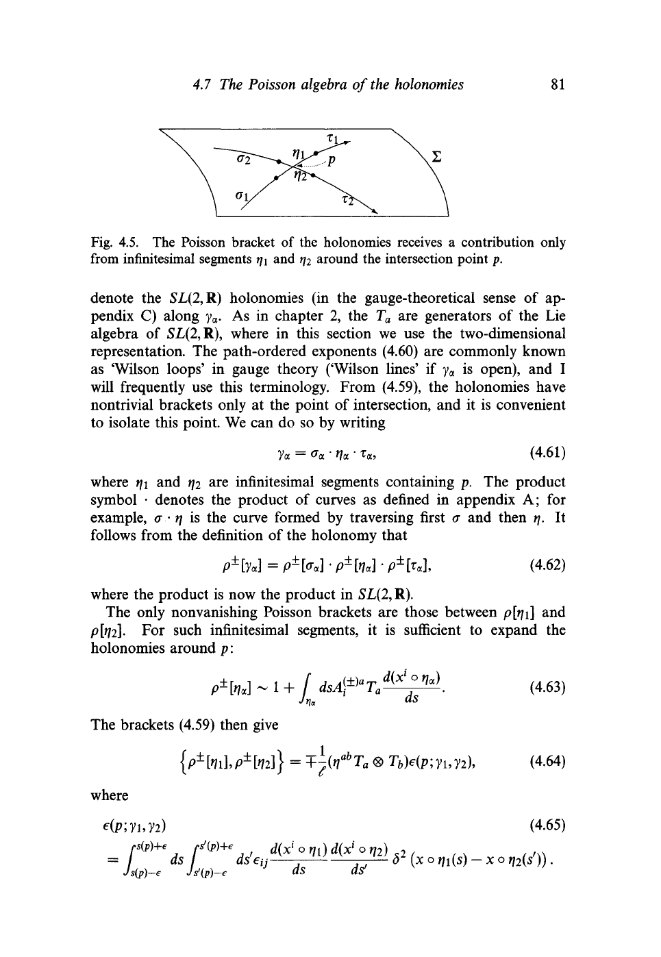
Now consider two paths y\ and 72 intersecting at a point p, as shown

in figure 4.5, and let

j =

exp y

A^Tadx^

(4.60)

Cambridge Books Online © Cambridge University Press, 2009

4.7 The Poisson algebra of the holonomies 81

Fig. 4.5. The Poisson bracket of the holonomies receives a contribution only

from infinitesimal segments r\\ and r\i around the intersection point p.

denote the SL(2,R) holonomies (in the gauge-theoretical sense of ap-

pendix C) along y

. As in chapter 2, the T

are generators of the Lie

algebra of SX(2,R), where in this section we use the two-dimensional

representation. The path-ordered exponents (4.60) are commonly known

as 'Wilson loops' in gauge theory ('Wilson lines' if y

is open), and I

will frequently use this terminology. From (4.59), the holonomies have

nontrivial brackets only at the point of intersection, and it is convenient

to isolate this point. We can do so by writing

= °*

•

T«,

(4.61)

where r\\ and r\2 are infinitesimal segments containing p. The product

symbol • denotes the product of curves as defined in appendix A; for

example, a

•

is the curve formed by traversing first a and then r\. It

follows from the definition of the holonomy that

I +

-i

(A (\

where the product is now the product in

SL(2,

R).

The only nonvanishing Poisson brackets are those between p[t]\] and

p[f]2]' For such infinitesimal segments, it is sufficient to expand the

holonomies around p:

The brackets (4.59) then give

where

)e(p;y

(4.63)

(4.64)

s(p)+e

Js(p)-€

(4.65)

;

o tn(s) - x o ri

(s')).

Cambridge Books Online © Cambridge University Press, 2009

Geometric structures

and

Chern-Simons theory

is a

standard result

differential geometry that e(p; 71,72)

is the

oriented

intersection number

and 72 at p, a

topological invariant equal

to ±1

depending

whether

the the

dyad formed

by the two

tangent vectors

right-

left-handed.

Restoring

the

remaining factors

a and

and

using

the

identity

= ~8p% +

5£

(4.66)

for

the

two-dimensional representation

SL(2,

R),

obtain

(4.67)

(Hyi^NpHyifq

•

]

Qp±[a

•

or symbolically,

For curves that intersect

more than

one

point,

must

sum a

relation-

ship

this form over

all

intersections.

Let

us now

consider

a set of

closed loops

that represent elements

7Ti(S,*).

The

holonomies p

]

are not yet

gauge-invariant observables:

under

gauge transformation

(±) _

(±)-i

(±)

g^-

Ag^\

(4.69)

we have

]

(±)

(*rV

(±)

(*)

(4.70)

where

* is the

base point. This noninvariance

is a

reflection

of the

equiv-

alence relation (4.21)

for

holonomies that differ

overall conjugation.

The traces

[y«]

\Tr

[y«l (4.71)

however,

are

gauge invariant,

and

provide

(overcomplete)

set of

vari-

ables

on the

classical phase space. Their Poisson brackets

are

easily

obtained from (4.67).

In particular, suppose

two

loops

71 and 72

intersect only

at the

base

point.

The

trace

(4.67) then gives

(^[71

•

yi]

- )

(4.72)

Cambridge Books Online © Cambridge University Press, 2009

4.7 The Poisson algebra of the holonomies 83

For loops with more than one intersection, the algebra is somewhat more

complicated; if the intersections are at points pu equation (4.72) must be

replaced by

(4.73)

In this expression, the symbol

•,•

denotes the product of

curves,

as described

in appendix A, with pi treated as the base point; that is, yi •/ 72 is the

loop obtained by starting at p\ and first traversing yi, then 72- Because

of this composition, it is difficult to find small subalgebras of the algebra

of holonomies that close under Poisson brackets. However, Nelson and

Regge have succeeded in constructing a small but complete (actually

overcomplete) set of holonomies on a surface of arbitrary genus that form

a closed algebra [206, 207, 208].

For the torus, in particular, the geometric structure is completely deter-

mined by a closed subalgebra of three holonomies. Let y\ and y2 be two

independent circumferences, and denote the traces

/^[yi],

#^2],

[yi ' yi\ as iJ^, ftjr,

d #i2- We then have

{i?j-,jR2"j = H—y-(Ri2

^f^2~)

" cyclical permutations,

€

(4.74)

where I have restored the gravitational constant. The six traces R^- are,

in fact, overcomplete - the space of geometric structures on the torus is

only four-dimensional. To understand this overcompleteness, consider the

cubic polynomials

-Tr (/ -p

[n]p

[y2]p

[yr

[72"

]) , (4.75)

where the last equality follows from the identity

A+A~

=ITrA

(4.76)

for matrices A e SL(2,

R).

The F

vanish classically, since the fundamental

group of the torus satisfies the relation

and the conditions F* = 0 thus provide two relations among the six R£.

For the torus, we have already obtained an explicit representation (4.33)

for the holonomies in terms of a set of coordinates r± on the space of

Geometric structures

and

Chern-Simons theory

geometric structures. It is now fairly easy to show that the symplectic struc-

ture (4.39) for these coordinates is equivalent to the symplectic structure

of equation (4.74), and that the polynomials F

vanish when expressed in

these coordinates, confirming the consistency of our descriptions.

Although the brackets (4.73) were derived in the context of general

relativity, it is interesting to note that they occur as well in the general

theory of Riemann surfaces. The moduli space

Jf = Homo(^i(2),SO(2,1))/ ~ (4.78)

of section 3 admits a natural symplectic structure, and in investigating

that structure Goldman has found a set of Poisson brackets equivalent to

those of (2+l)-dimensional gravity

[129].

A similar set of relations occurs

when one considers homomorphisms from ni(L) into an arbitrary group

G, although for

SL(2, R)

an additional set of relations holds: it follows

from (4.76) that TrAB + TrAB~

= TrATrB, and hence

RHvilRHyi] = \ (RHyi

•

]

+ RHvi

•

])

•

(4.79)

Relations of this type are known as Mandelstam constraints.

In the case of a vanishing cosmological constant, a similar algebra can

be found, using an appropriate matrix representation of ISO (2,1)

[188].

is often more useful to choose a slightly different set of

variables,

however,

to make use of the cotangent bundle structure of the space of geometric

structures. (Recall that this structure occurred only for A = 0.) Let

(4.80)

be the holonomy of the

SO (2,1)

connection one-form

around a loop

y, with base point x. As before, the #

are a set of generators of

the Lie algebra of SO

(2,1);

it is traditional to use the two-dimensional

representation of SU(2), the covering space of SO(2,1). The Ashtekar-

Rovelli-Smolin loop variables are then [11, 13]

:] (4.81)

and

T'[y] = fTr{p

[y,x(s)]e

(y(s))/

(4.82)

T°[y] may be recognized as the

ISO (2,1)

holonomy in the representation

= 0. T

[y] is essentially a cotangent vector to T°[y]. Indeed, given a

4.7

The

Poisson algebra

the holonomies

family co

(t)

flat connections,

the

derivative

(4.81) yields

2^-T°[y](t)

= [Tr

(po(t)[y,x(s)] ^-co

(t)(y(

))/

)

Jy \ dt )

and we saw

chapter

that triads

may be interpreted

cotangent

vectors dco

/dt to the space

flat connections.

The variables

T°

and

obey

closed Poisson algebra. The compu-

tation

the relevant brackets

nearly identical

the computation for

SL(2,R) described above; for

set of intersection points pu we obtain

{T°[yilT°[y

]}=0

frpir -i ri->0

"I 1 \ ^ / \

/rpOr

rriOr

—li\

|T [yi],T

= -^

l^^Puy^yi) [T

[yi -,- 72]

[yi

'iy

])

[yi],T

5^^(Pi;71,72)

(^[yi

-,-72]

T^yi

-/y^

]),

(4.84)

where

the

product

was

defined

page

83. T°[y] and T

[y]

also obey

set of

Mandelstam constraints analogous

(4.79):

T°[yi]T°[y

]

= -

(r°[yi

•

]

T°[yi

•

-^/l

(4.85)

along with

the

identities

T°[0]

1, T°[y]

T^y-

], T°[

•

]

T°[y

•

]

[0]=0,

[y]

[y-

T^yi

•

]

•

yi]. (4.86)

Once again,

the

composition

loops

(4.84)

and

(4.85) makes

difficult

extract

finite-dimensional

set of

observables that parametrize

the phase space

Jf. As

usual, however,

if Z has the

topology

of a

torus,

the mathematics simplifies drastically.

discussed

appendix

A, the

two generators

y\ and y

n\(T

) commute,

so any

curve

on the

torus

homotopic

curve

•

. Any

homotopy class

may

thus

labeled

two

integers

m and n, the

winding numbers

in the

and

directions.

may

therefore think

of T°

and

being functions

these

two

integers.

Moreover, using

the

explicit expressions (3.76)

and

(3.78)

for the

triad

and spin connection

[0,1]

we can

compute these functions