Brealey, Myers. Principles of Corporate Finance. 7th edition

Подождите немного. Документ загружается.

Brealey−Meyers:

Principles of Corporate

Finance, Seventh Edition

I. Value 5. Why Net Prsnt Value

Leads to Better

Investments Decisions

than Other Criteria

Companies, 2003

Some companies discount the cash flows before they compute the payback pe-

riod. The discounted-payback rule asks, How many periods does the project have

to last in order to make sense in terms of net present value? This modification to

the payback rule surmounts the objection that equal weight is given to all flows be-

fore the cutoff date. However, the discounted-payback rule still takes no account

of any cash flows after the cutoff date.

96 PART I

Value

5.3 INTERNAL (OR DISCOUNTED-CASH-FLOW)

RATE OF RETURN

Whereas payback and return on book are ad hoc measures, internal rate of return

has a much more respectable ancestry and is recommended in many finance texts.

If, therefore, we dwell more on its deficiencies, it is not because they are more nu-

merous but because they are less obvious.

In Chapter 2 we noted that net present value could also be expressed in terms of

rate of return, which would lead to the following rule: “Accept investment oppor-

tunities offering rates of return in excess of their opportunity costs of capital.” That

statement, properly interpreted, is absolutely correct. However, interpretation is

not always easy for long-lived investment projects.

There is no ambiguity in defining the true rate of return of an investment that

generates a single payoff after one period:

Alternatively, we could write down the NPV of the investment and find that dis-

count rate which makes NPV ⫽ 0.

implies

Of course C

is the payoff and ⫺C

is the required investment, and so our two equa-

tions say exactly the same thing. The discount rate that makes NPV ⫽ 0 is also the rate

of return.

Unfortunately, there is no wholly satisfactory way of defining the true rate of re-

turn of a long-lived asset. The best available concept is the so-called discounted-

cash-flow (DCF) rate of return or internal rate of return (IRR). The internal rate

of return is used frequently in finance. It can be a handy measure, but, as we shall

see, it can also be a misleading measure. You should, therefore, know how to cal-

culate it and how to use it properly.

The internal rate of return is defined as the rate of discount which makes NPV

⫽ 0. This means that to find the IRR for an investment project lasting T years, we

must solve for IRR in the following expression:

NPV ⫽ C

⫹

1 ⫹ IRR

⫹

11 ⫹ IRR2

⫹

…

⫹

11 ⫹ IRR2

⫽ 0

Discount rate ⫽

⫺ C

⫺ 1

NPV ⫽ C

⫹

1 ⫹ discount rate

⫽ 0

Rate of return ⫽

payoff

investment

⫺ 1

Brealey−Meyers:

Principles of Corporate

Finance, Seventh Edition

I. Value 5. Why Net Prsnt Value

Leads to Better

Investments Decisions

than Other Criteria

Companies, 2003

Actual calculation of IRR usually involves trial and error. For example, consider

a project that produces the following flows:

CHAPTER 5

Why Net Present Value Leads to Better Investment Decisions Than Other Criteria 97

Cash Flows ($)

–4,000 ⫹2,000 ⫹4,000

The internal rate of return is IRR in the equation

Let us arbitrarily try a zero discount rate. In this case NPV is not zero but ⫹$2,000:

The NPV is positive; therefore, the IRR must be greater than zero. The next step

might be to try a discount rate of 50 percent. In this case net present value is –$889:

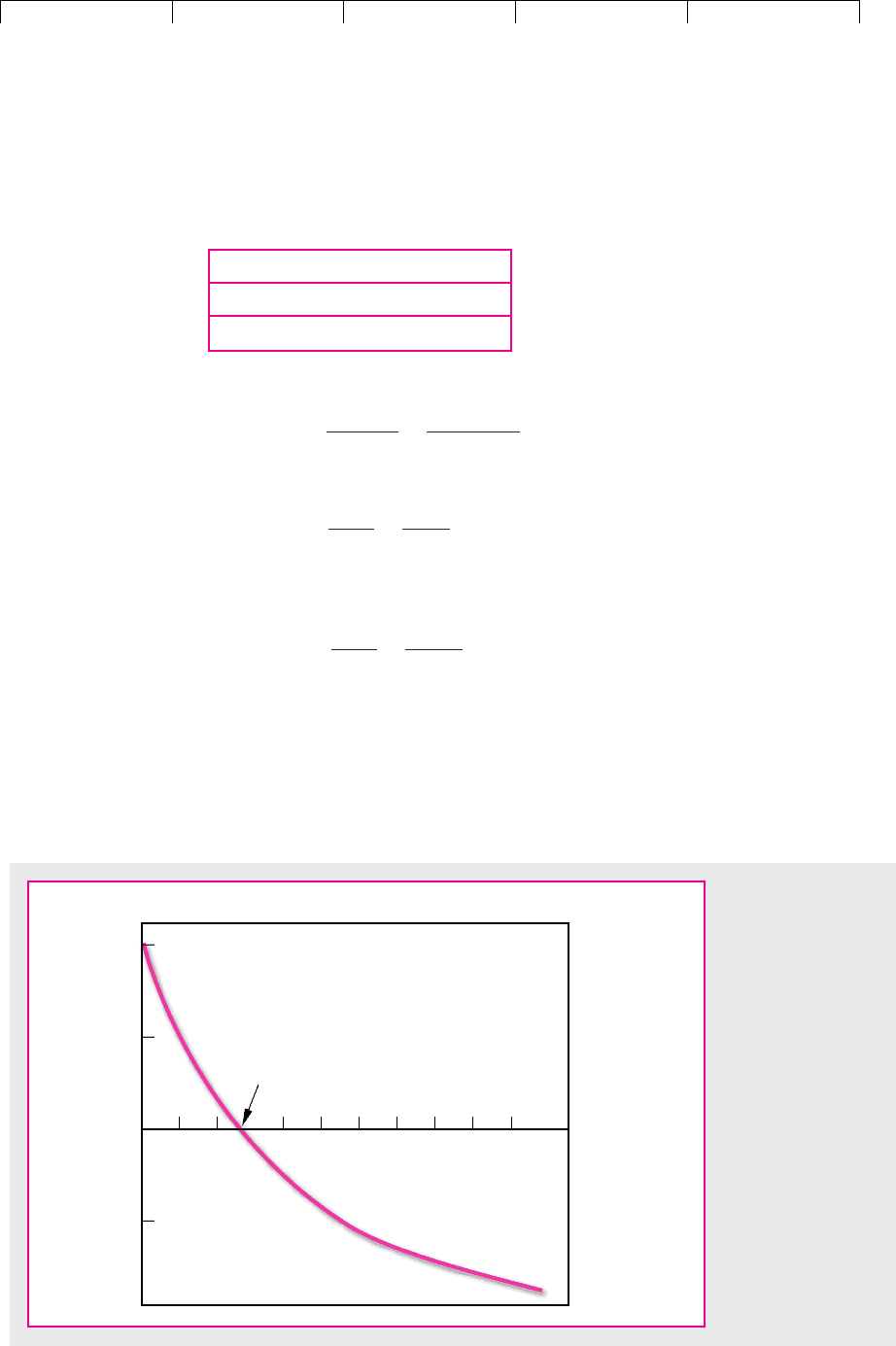
The NPV is negative; therefore, the IRR must be less than 50 percent. In Figure 5.2

we have plotted the net present values implied by a range of discount rates. From

this we can see that a discount rate of 28 percent gives the desired net present value

of zero. Therefore IRR is 28 percent.

The easiest way to calculate IRR, if you have to do it by hand, is to plot three or

four combinations of NPV and discount rate on a graph like Figure 5.2, connect the

NPV ⫽⫺4,000 ⫹

2,000

1.50

⫹

4,000

11.502

⫽⫺$889

NPV ⫽⫺4,000 ⫹

2,000

1.0

⫹

4,000

11.02

⫽⫹$2,000

NPV ⫽⫺4,000 ⫹

2,000

1 ⫹ IRR

⫹

4,000

11 ⫹ IRR2

⫽ 0

–2,000

Net present value, dollars

Discount rate,

percent

+1,000

–1,000

+2,000

100

9080706050402010

IRR = 28 percent

FIGURE 5.2

This project costs

$4,000 and then

produces cash inflows

of $2,000 in year 1

and $4,000 in year 2.

Its internal rate of

return (IRR) is 28

percent, the rate of

discount at which

NPV is zero.

Brealey−Meyers:

Principles of Corporate

Finance, Seventh Edition

I. Value 5. Why Net Prsnt Value

Leads to Better

Investments Decisions

than Other Criteria

Companies, 2003

points with a smooth line, and read off the discount rate at which NPV = 0. It is of

course quicker and more accurate to use a computer or a specially programmed

calculator, and this is what most financial managers do.

Now, the internal rate of return rule is to accept an investment project if the op-

portunity cost of capital is less than the internal rate of return. You can see the rea-

soning behind this idea if you look again at Figure 5.2. If the opportunity cost of

capital is less than the 28 percent IRR, then the project has a positive NPV when dis-

counted at the opportunity cost of capital. If it is equal to the IRR, the project has a

zero NPV. And if it is greater than the IRR, the project has a negative NPV. Therefore,

when we compare the opportunity cost of capital with the IRR on our project, we

are effectively asking whether our project has a positive NPV. This is true not only

for our example. The rule will give the same answer as the net present value rule

whenever the NPV of a project is a smoothly declining function of the discount rate.

Many firms use internal rate of return as a criterion in preference to net present

value. We think that this is a pity. Although, properly stated, the two criteria are

formally equivalent, the internal rate of return rule contains several pitfalls.

Pitfall 1—Lending or Borrowing?

Not all cash-flow streams have NPVs that decline as the discount rate increases.

Consider the following projects A and B:

98 PART I

Value

Here is a word of caution: Some people confuse the internal rate of return and the opportunity cost of

capital because both appear as discount rates in the NPV formula. The internal rate of return is a prof-

itability measure that depends solely on the amount and timing of the project cash flows. The opportu-

nity cost of capital is a standard of profitability for the project which we use to calculate how much the

project is worth. The opportunity cost of capital is established in capital markets. It is the expected rate

of return offered by other assets equivalent in risk to the project being evaluated.

Cash Flows ($)

Project C

IRR NPV at 10%

A –1,000 ⫹1,500 ⫹50% ⫹364

B ⫹1,000 –1,500 ⫹50% –364

Each project has an IRR of 50 percent. (In other words, –1,000 ⫹ 1,500/1.50 ⫽ 0 and

⫹ 1,000 – 1,500/1.50 ⫽ 0.)

Does this mean that they are equally attractive? Clearly not, for in the case of A,

where we are initially paying out $1,000, we are lending money at 50 percent; in the

case of B, where we are initially receiving $1,000, we are borrowing money at 50 per-

cent. When we lend money, we want a high rate of return; when we borrow money,

we want a low rate of return.

If you plot a graph like Figure 5.2 for project B, you will find that NPV increases

as the discount rate increases. Obviously the internal rate of return rule, as we

stated it above, won’t work in this case; we have to look for an IRR less than the op-

portunity cost of capital.

This is straightforward enough, but now look at project C:

Cash Flows ($)

Project C

IRR NPV at 10%

C ⫹1,000 –3,600 ⫹4,320 –1,728 ⫹20% –.75

Brealey−Meyers:

Principles of Corporate

Finance, Seventh Edition

I. Value 5. Why Net Prsnt Value

Leads to Better

Investments Decisions

than Other Criteria

Companies, 2003

It turns out that project C has zero NPV at a 20 percent discount rate. If the oppor-

tunity cost of capital is 10 percent, that means the project is a good one. Or does it?

In part, project C is like borrowing money, because we receive money now and pay

it out in the first period; it is also partly like lending money because we pay out

money in period 1 and recover it in period 2. Should we accept or reject? The only

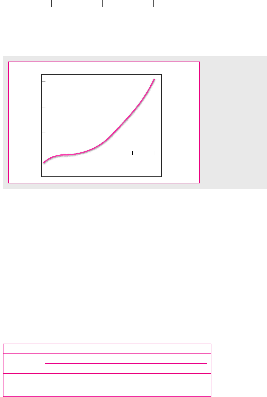
way to find the answer is to look at the net present value. Figure 5.3 shows that the

NPV of our project increases as the discount rate increases. If the opportunity cost

of capital is 10 percent (i.e., less than the IRR), the project has a very small negative

NPV and we should reject.

Pitfall 2—Multiple Rates of Return

In most countries there is usually a short delay between the time when a com-

pany receives income and the time it pays tax on the income. Consider the case

of Albert Vore, who needs to assess a proposed advertising campaign by the veg-

etable canning company of which he is financial manager. The campaign in-

volves an initial outlay of $1 million but is expected to increase pretax profits by

$300,000 in each of the next five periods. The tax rate is 50 percent, and taxes are

paid with a delay of one period. Thus the expected cash flows from the invest-

ment are as follows:

CHAPTER 5

Why Net Present Value Leads to Better Investment Decisions Than Other Criteria 99

–20

Net present value, dollars

Discount rate,

percent

+20

1008060

+40

+60

FIGURE 5.3

The NPV of project C

increases as the discount

rate increases.

Cash Flows ($ thousands)

Period

0123456

Pretax flow –1,000 ⫹300 ⫹300 ⫹300 ⫹300 ⫹300

Tax ⫹500 –150 –150 –150 –150 –150

Net flow –1,000 ⫹800 ⫹150 ⫹150 ⫹150 ⫹150 –150

Note: The $1 million outlay in period 0 reduces the company’s taxes in period 1 by $500,000; thus we enter ⫹500

in year 1.

Brealey−Meyers:

Principles of Corporate

Finance, Seventh Edition

I. Value 5. Why Net Prsnt Value

Leads to Better

Investments Decisions

than Other Criteria

Companies, 2003

Mr. Vore calculates the project’s IRR and its NPV as follows:

100 PART I

Value

–1,000

Net present value, thousands of dollars

Discount rate,

percent

500

–500

1,500

–25 0 25 50

IRR = –50 percent

1,000

IRR = 15.2 percent

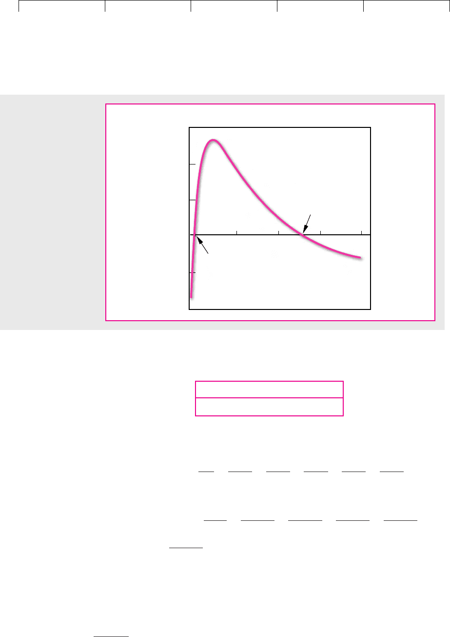
FIGURE 5.4

The advertising

campaign has two

internal rates of return.

NPV ⫽ 0 when the

discount rate is ⫺50

percent and when it is

⫹15.2 percent.

IRR (%) NPV at 10%

⫺50 and 15.2 74.9 or $74,900

Note that there are two discount rates that make NPV = 0. That is, each of the fol-

lowing statements holds:

and

In other words, the investment has an IRR of both –50 and 15.2 percent. Figure 5.4

shows how this comes about. As the discount rate increases, NPV initially rises and

then declines. The reason for this is the double change in the sign of the cash-flow

stream. There can be as many different internal rates of return for a project as there

are changes in the sign of the cash flows.

⫺

150

11.1522

⫽ 0

NPV ⫽⫺1,000 ⫹

800

1.152

⫹

150

11.1522

⫹

150

11.1522

⫹

150

11.1522

⫹

150

11.1522

NPV ⫽⫺1,000 ⫹

800

.50

⫹

150

1.502

⫹

150

1.502

⫹

150

1.502

⫹

150

1.502

⫺

150

1.502

⫽ 0

By Descartes’s “rule of signs” there can be as many different solutions to a polynomial as there are

changes of sign. For a discussion of the problem of multiple rates of return, see J. H. Lorie and L. J. Sav-

age, “Three Problems in Rationing Capital,” Journal of Business 28 (October 1955), pp. 229–239; and E.

Solomon, “The Arithmetic of Capital Budgeting,” Journal of Business 29 (April 1956), pp. 124–129.

Brealey−Meyers:

Principles of Corporate

Finance, Seventh Edition

I. Value 5. Why Net Prsnt Value

Leads to Better

Investments Decisions

than Other Criteria

Companies, 2003

In our example the double change in sign was caused by a lag in tax payments,

but this is not the only way that it can occur. For example, many projects involve

substantial decommissioning costs. If you strip-mine coal, you may have to invest

large sums to reclaim the land after the coal is mined. Thus a new mine creates an

initial investment (negative cash flow up front), a series of positive cash flows, and

an ending cash outflow for reclamation. The cash-flow stream changes sign twice,

and mining companies typically see two IRRs.

As if this is not difficult enough, there are also cases in which no internal rate

of return exists. For example, project D has a positive net present value at all dis-

count rates:

CHAPTER 5

Why Net Present Value Leads to Better Investment Decisions Than Other Criteria 101

Companies sometimes get around the problem of multiple rates of return by discounting the later cash

flows back at the cost of capital until there remains only one change in the sign of the cash flows. Amod-

ified internal rate of return can then be calculated on this revised series. In our example, the modified IRR

is calculated as follows:

1. Calculate the present value of the year 6 cash flow in year 5:

PV in year 5 = –150/1.10 = –136.36

2. Add to the year 5 cash flow the present value of subsequent cash flows:

+ PV(subsequent cash flows) = 150 – 136.36 = 13.64

3. Since there is now only one change in the sign of the cash flows, the revised series has a unique

rate of return, which is 15 percent:

Since the modified IRR of 15 percent is greater than the cost of capital (and the initial cash flow

is negative), the project has a positive NPV when valued at the cost of capital.

Of course, it would be much easier in such cases to abandon the IRR rule and just calculate

project NPV.

NPV ⫽⫺1,000 ⫹

800

1.15

⫹

150

1.15

⫹

150

1.15

⫹

150

1.15

⫹

13.64

1.15

⫽ 0

Cash Flows ($)

Project C

IRR (%) NPV at 10%

D ⫹1,000 –3,000 ⫹2,500 None ⫹339

A number of adaptations of the IRR rule have been devised for such cases. Not only

are they inadequate, but they also are unnecessary, for the simple solution is to use

net present value.

Pitfall 3—Mutually Exclusive Projects

Firms often have to choose from among several alternative ways of doing the same

job or using the same facility. In other words, they need to choose from among mu-

tually exclusive projects. Here too the IRR rule can be misleading.

Consider projects E and F:

Cash Flows ($)

Project C

IRR (%) NPV at 10%

E –10,000 ⫹20,000 100 ⫹ 8,182

F –20,000 ⫹35,000 75 ⫹11,818

Brealey−Meyers:

Principles of Corporate

Finance, Seventh Edition

I. Value 5. Why Net Prsnt Value

Leads to Better

Investments Decisions

than Other Criteria

Companies, 2003

Perhaps project E is a manually controlled machine tool and project F is the same

tool with the addition of computer control. Both are good investments, but F has

the higher NPV and is, therefore, better. However, the IRR rule seems to indicate

that if you have to choose, you should go for E since it has the higher IRR. If you

follow the IRR rule, you have the satisfaction of earning a 100 percent rate of re-

turn; if you follow the NPV rule, you are $11,818 richer.

You can salvage the IRR rule in these cases by looking at the internal rate of re-

turn on the incremental flows. Here is how to do it: First, consider the smaller proj-

ect (E in our example). It has an IRR of 100 percent, which is well in excess of the

10 percent opportunity cost of capital. You know, therefore, that E is acceptable.

You now ask yourself whether it is worth making the additional $10,000 invest-

ment in F. The incremental flows from undertaking F rather than E are as follows:

102 PART I

Value

Cash Flows ($)

Project C

IRR (%) NPV at 10%

F–E –10,000 ⫹15,000 50 ⫹3,636

The IRR on the incremental investment is 50 percent, which is also well in excess of

the 10 percent opportunity cost of capital. So you should prefer project F to project E.

Unless you look at the incremental expenditure, IRR is unreliable in ranking

projects of different scale. It is also unreliable in ranking projects which offer dif-

ferent patterns of cash flow over time. For example, suppose the firm can take proj-

ect G or project H but not both (ignore I for the moment):

You may, however, find that you have jumped out of the frying pan into the fire. The series of incre-

mental cash flows may involve several changes in sign. In this case there are likely to be multiple IRRs

and you will be forced to use the NPV rule after all.

Cash Flows ($)

IRR NPV

Project C

Etc. (%) at 10%

G –9,000 ⫹6,000 ⫹5,000 ⫹4,000 0 0 . . . 33 3,592

H –9,000 ⫹1,800 ⫹1,800 ⫹1,800 ⫹1,800 ⫹1,800 . . . 20 9,000

I –6,000 ⫹1,200 ⫹1,200 ⫹1,200 ⫹1,200 . . . 20 6,000

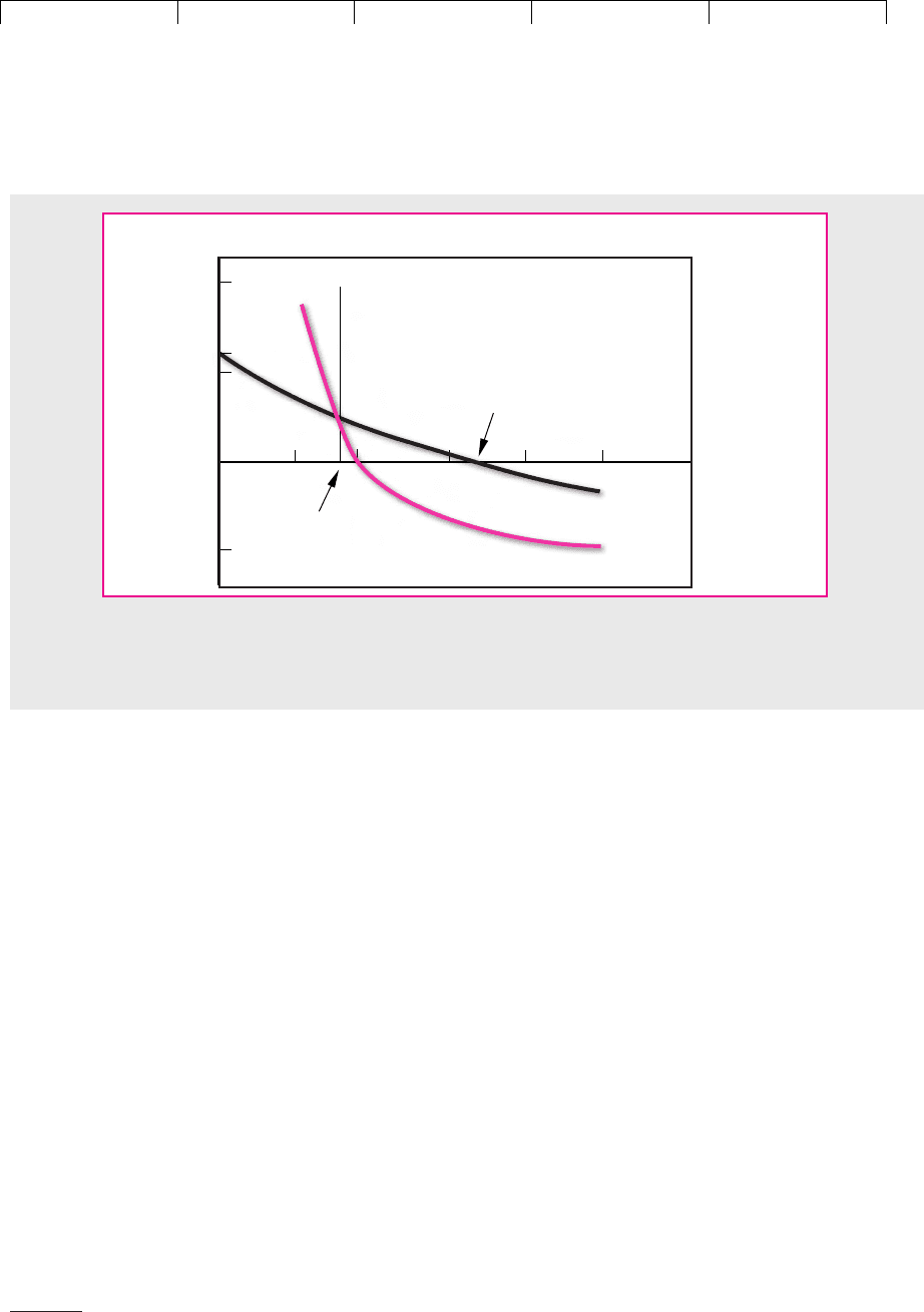
Project G has a higher IRR, but project H has the higher NPV. Figure 5.5 shows why

the two rules give different answers. The blue line gives the net present value of

project G at different rates of discount. Since a discount rate of 33 percent produces

a net present value of zero, this is the internal rate of return for project G. Similarly,

the burgundy line shows the net present value of project H at different discount

rates. The IRR of project H is 20 percent. (We assume project H’s cash flows con-

tinue indefinitely.) Note that project H has a higher NPV so long as the opportu-

nity cost of capital is less than 15.6 percent.

The reason that IRR is misleading is that the total cash inflow of project H is

larger but tends to occur later. Therefore, when the discount rate is low, H has the

higher NPV; when the discount rate is high, G has the higher NPV. (You can see

from Figure 5.5 that the two projects have the same NPV when the discount rate is

15.6 percent.) The internal rates of return on the two projects tell us that at a dis-

count rate of 20 percent H has a zero NPV (IRR ⫽ 20 percent) and G has a positive

Brealey−Meyers:

Principles of Corporate

Finance, Seventh Edition

I. Value 5. Why Net Prsnt Value

Leads to Better

Investments Decisions

than Other Criteria

Companies, 2003

NPV. Thus if the opportunity cost of capital were 20 percent, investors would place

a higher value on the shorter-lived project G. But in our example the opportunity

cost of capital is not 20 percent but 10 percent. Investors are prepared to pay rela-

tively high prices for longer-lived securities, and so they will pay a relatively high

price for the longer-lived project. At a 10 percent cost of capital, an investment in

H has an NPV of $9,000 and an investment in G has an NPV of only $3,592.

This is a favorite example of ours. We have gotten many businesspeople’s reac-

tion to it. When asked to choose between G and H, many choose G. The reason

seems to be the rapid payback generated by project G. In other words, they believe

that if they take G, they will also be able to take a later project like I (note that I can

be financed using the cash flows from G), whereas if they take H, they won’t have

money enough for I. In other words they implicitly assume that it is a shortage of

capital which forces the choice between G and H. When this implicit assumption is

brought out, they usually admit that H is better if there is no capital shortage.

But the introduction of capital constraints raises two further questions. The first

stems from the fact that most of the executives preferring G to H work for firms

that would have no difficulty raising more capital. Why would a manager at IBM,

say, choose G on the grounds of limited capital? IBM can raise plenty of capital and

can take project I regardless of whether G or H is chosen; therefore I should not af-

fect the choice between G and H. The answer seems to be that large firms usually

impose capital budgets on divisions and subdivisions as a part of the firm’s plan-

ning and control system. Since the system is complicated and cumbersome, the

CHAPTER 5

Why Net Present Value Leads to Better Investment Decisions Than Other Criteria 103

–5,000

Net present value, dollars

Discount rate,

percent

Project G

Project H

+5,000

5040

3020

15.6

33.3

+6,000

+10,000

FIGURE 5.5

The IRR of project G exceeds that of project H, but the NPV of project G is higher only if the

discount rate is greater than 15.6 percent.

It is often suggested that the choice between the net present value rule and the internal rate of return

rule should depend on the probable reinvestment rate. This is wrong. The prospective return on another

independent investment should never be allowed to influence the investment decision. For a discussion

of the reinvestment assumption see A. A. Alchian, “The Rate of Interest, Fisher’s Rate of Return over

Cost and Keynes’ Internal Rate of Return,” American Economic Review 45 (December 1955), pp. 938–942.

Brealey−Meyers:

Principles of Corporate

Finance, Seventh Edition

I. Value 5. Why Net Prsnt Value

Leads to Better

Investments Decisions

than Other Criteria

Companies, 2003

budgets are not easily altered, and so they are perceived as real constraints by mid-

dle management.

The second question is this. If there is a capital constraint, either real or self-

imposed, should IRR be used to rank projects? The answer is no. The problem in

this case is to find that package of investment projects which satisfies the capital

constraint and has the largest net present value. The IRR rule will not identify this

package. As we will show in the next section, the only practical and general way

to do so is to use the technique of linear programming.

When we have to choose between projects G and H, it is easiest to compare the

net present values. But if your heart is set on the IRR rule, you can use it as long as

you look at the internal rate of return on the incremental flows. The procedure is

exactly the same as we showed above. First, you check that project G has a satis-

factory IRR. Then you look at the return on the additional investment in H.

104 PART I

Value

Cash Flows ($)

IRR NPV

Project C

Etc. (%) at 10%

H–G 0 –4,200 –3,200 –2,200 ⫹1,800 ⫹1,800 ⋅⋅⋅ 15.6 ⫹5,408

The IRR on the incremental investment in H is 15.6 percent. Since this is greater

than the opportunity cost of capital, you should undertake H rather than G.

Pitfall 4—What Happens When We Can’t Finesse

the Term Structure of Interest Rates?

We have simplified our discussion of capital budgeting by assuming that the op-

portunity cost of capital is the same for all the cash flows, C

, C

, etc. This is not

the right place to discuss the term structure of interest rates, but we must point out

certain problems with the IRR rule that crop up when short-term interest rates are

different from long-term rates.

Remember our most general formula for calculating net present value:

In other words, we discount C

at the opportunity cost of capital for one year, C

at the

opportunity cost of capital for two years, and so on. The IRR rule tells us to accept a

project if the IRR is greater than the opportunity cost of capital. But what do we do

when we have several opportunity costs? Do we compare IRR with r

, r

, . . .? Ac-

tually we would have to compute a complex weighted average of these rates to ob-

tain a number comparable to IRR.

What does this mean for capital budgeting? It means trouble for the IRR rule when-

ever the term structure of interest rates becomes important.

In a situation where it is

important, we have to compare the project IRR with the expected IRR (yield to matu-

rity) offered by a traded security that (1) is equivalent in risk to the project and (2) of-

fers the same time pattern of cash flows as the project. Such a comparison is easier said

than done. It is much better to forget about IRR and just calculate NPV.

NPV ⫽ C

⫹

1 ⫹ r

⫹

11 ⫹ r

⫹

11 ⫹ r

⫹

…

The source of the difficulty is that the IRR is a derived figure without any simple economic interpreta-

tion. If we wish to define it, we can do no more than say that it is the discount rate which applied to all

cash flows makes NPV = 0. The problem here is not that the IRR is a nuisance to calculate but that it is

not a useful number to have.

Brealey−Meyers:

Principles of Corporate

Finance, Seventh Edition

I. Value 5. Why Net Prsnt Value

Leads to Better

Investments Decisions

than Other Criteria

Companies, 2003

Many firms use the IRR, thereby implicitly assuming that there is no difference

between short-term and long-term rates of interest. They do this for the same rea-

son that we have so far finessed the term structure: simplicity.

The Verdict on IRR

We have given four examples of things that can go wrong with IRR. We spent much

less space on payback or return on book. Does this mean that IRR is worse than the

other two measures? Quite the contrary. There is little point in dwelling on the de-

ficiencies of payback or return on book. They are clearly ad hoc measures which of-

ten lead to silly conclusions. The IRR rule has a much more respectable ancestry. It

is a less easy rule to use than NPV, but, used properly, it gives the same answer.

Nowadays few large corporations use the payback period or return on book as

their primary measure of project attractiveness. Most use discounted cash flow or

“DCF,” and for many companies DCF means IRR, not NPV. We find this puzzling, but

it seems that IRR is easier to explain to nonfinancial managers, who think they know

what it means to say that “Project G has a 33 percent return.” But can these managers

use IRR properly? We worry particularly about Pitfall 3. The financial manager never

sees all possible projects. Most projects are proposed by operating managers. Will the

operating managers’ proposals have the highest NPVs or the highest IRRs?

A company that instructs nonfinancial managers to look first at projects’ IRRs

prompts a search for high-IRR projects. It also encourages the managers to modify

projects so that their IRRs are higher. Where do you typically find the highest IRRs?

In short-lived projects requiring relatively little up-front investment. Such projects

may not add much to the value of the firm.

CHAPTER 5

Why Net Present Value Leads to Better Investment Decisions Than Other Criteria 105

In Chapter 9 we will look at some other cases in which it would be misleading to use the same discount

rate for both short-term and long-term cash flows.

5.4 CHOOSING CAPITAL INVESTMENTS

WHEN RESOURCES ARE LIMITED

Our entire discussion of methods of capital budgeting has rested on the proposi-

tion that the wealth of a firm’s shareholders is highest if the firm accepts every proj-

ect that has a positive net present value. Suppose, however, that there are limita-

tions on the investment program that prevent the company from undertaking all

such projects. Economists call this capital rationing. When capital is rationed, we

need a method of selecting the package of projects that is within the company’s re-

sources yet gives the highest possible net present value.

An Easy Problem in Capital Rationing

Let us start with a simple example. The opportunity cost of capital is 10 percent,

and our company has the following opportunities:

Cash Flows ($ millions)

Project C

NPV at 10%

A –10 ⫹30 ⫹521

B–5⫹5 ⫹20 16

C–5⫹5 ⫹15 12