Blanchet L., Spallicci A., Whiting B. (Eds.) Mass and Motion in General Relativity
Подождите немного. Документ загружается.

Constructing the Self-Force 311
tromagnetic self-force in flat spacetime is Dirac’s famous 1938 paper [4]. Dirac’s
construction was generalized to curved spacetime in 1960 by DeWitt and Brehme
[3]; a technical error in their work was corrected by Hobbs [7]. The gravitational
self-force was first computed in 1997 by Mino, Sasaki, and Tanaka [8]; a more di-
rect derivation (based on an axiomatic approach) was later provided by Quinn and
Wald [11]. Finally, the scalar self-force – the main topic of this lecture – was first
constructed in 2000 by Ted Quinn [10].
2 Geometric Elements
The construction of the self-force would be impossible without the introduction
of geometric tools that were first fashioned by Synge [13] and independently by
DeWitt and Brehme [3]. In this section I introduce the world function .x;x
0
/ and
the parallel propagator g
˛
˛
0
.x; x
0
/.
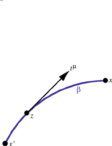
Let x and x
0
be two points in spacetime, and let us assume that they are suffi-
ciently close that there is a unique geodesic segment ˇ linking them. The segment
is described by the parametric relations z
./,inwhich is an affine parameter that
runs from 0 to 1;wehavethatz.0/ D x
0
and z.1/ D x. The vector t
WD d z
=d
is tangent to ˇ (Fig. 1).
The world function is defined by
.x;x
0
/ WD
1
2
Z
1
0
g
.z/t
t
d: (1)
It is numerically equal to half the squared geodesic distance between x and x
0
.When
<0the separation between x and x
0
is timelike, and when >0it is spacelike.
The equation .x;x
0
/ D 0 describes the light cones of each point; if x
0
is kept fixed
then .x/ D 0 describes the past and future light cones of x
0
; if instead x is kept
fixed then .x
0
/ D 0 describes the past and future light cones of x.
Fig. 1 Geodesic segment ˇ
between the spacetime points
x
0
and x. The vector t
is
tangent to this geodesic
312 E. Poisson
The world function can be differentiated with respect to each argument. It can be
shown (LRR Section 2.1.2) that
˛
0
WD r
˛
0
.x;x
0
/ (2)
is a vector at x
0
that is proportional to t
evaluated at that point. I use the convention
that primed indices refer to the point x
0
, while unprimed indices refer to x. It can
also be shown that its length is given by
g
˛
0
ˇ
0
˛
0
ˇ
0
D 2I (3)
the length of
˛
0
therefore measures the geodesic distance between the two points.
Because the vector points from x
0
to x, we have a covariant notion of a displacement
vector between the two points.
The parallel propagator takes a vector A
˛
0
at x
0
and moves it to x by parallel
transport on the geodesic segment ˇ. We express this operation as
A
˛
.x/ D g
˛
˛
0
.x; x
0
/A
˛
0
.x
0
/; (4)
in which A
˛
is the resulting vector at x. The operation is easily generalized to dual
vectors and other types of tensors (LRR Section 2.3).
The world function and the parallel propagator can be employed in the construc-
tion of a Taylor expansion of a tensor about a reference point x
0
. Suppose that we
have a tensor field A
˛ˇ
.x/ and that we wish to express it as an expansion in pow-
ers of the displacement away from x
0
. The role of the deviation vector is played by
˛
0
, and the expansion coefficients will be ordinary tensors at x
0
. We might write
something like
A
˛
0
ˇ
0
C A
˛
0
ˇ
0
0
.
0
/ C
1
2
A
˛
0
ˇ
0
0
ı
0
.
0
/.
ı
0
/ C;
but this defines a tensor at x
0
, not x. To get a proper expression for A
˛ˇ
.x/ we must
also involve the parallel propagator, and we write
A
˛ˇ
D g
˛
˛
0
g
ˇ
ˇ
0
A
˛
0
ˇ
0
A
˛
0
ˇ
0
0
0
C
1
2
A
˛
0
ˇ
0
0
ı
0
0
ı
0
C
: (5)
Having postulated this form for the expansion, the expansion coefficients A
˛
0
ˇ
0
,
A
˛
0
ˇ
0
0
, and so on can be computed by repeatedly differentiating the tensor field and
evaluating the results in the limit x ! x
0
(see LRR Section 2.4). For example,
A
˛
0
ˇ
0
D lim A
˛ˇ
, as we might expect.
3 Coordinate Systems
Self-force computations are best carried out using covariant methods. It is conve-
nient, however, to display the results in a coordinate system that is well suited
to the description of a neighborhood of the world line . In this transcription
Constructing the Self-Force 313
it is advantageous to keep the coordinates in a close correspondence with the
geometric objects (such as
˛
0
) that appear in the covariant expressions. I find that
two coordinate systems are particularly useful in this context: the Fermi normal
coordinates .t; x
a
D s!
a
/,andtheretarded null-cone coordinates .u;x
a
D r˝
a
/.
A third coordinate system, known as the Thorne–Hartle–Zhang coordinates
[14, 15], has also appeared in the self-force literature – they are the favored choice
of the Florida group led by Steve Detweiler and Bernard Whiting (see, e.g., Ref. [1]).
The THZ coordinates are a variant of the Fermi coordinates, and they have some
nice properties. But I find them less convenient to deal with than the Fermi or
retarded coordinates, because they do not seem to possess a simple covariant defi-
nition. (The THZ coordinates may enjoy the mild Florida winters, but they are not
robust enough to endure the tougher Canadian winters.) I shall not discuss the THZ
coordinates here.
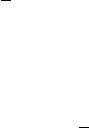
The Fermi and retarded coordinates share a basic geometrical construction on
the world line. At each point on we erect a basis .u
;e
a
/ of orthonormal vec-
tors. The timelike vector u
is the particle’s velocity vector, and it is tangent to the
world line. The spatial unit vectors e
a
are labeled with the index a D 1; 2; 3,and
they are all orthogonal to u
; they are also mutually orthogonal. The vectors are
transported on so as to preserve their orthonormality properties. If the world line
is a geodesic, then we might take the vectors e
a
to be parallel transported on .
If instead the world line is accelerated, then we might take the spatial vectors to
be Fermi–Walker transported on the world line (LRR Section 3.2.1). The tetrad of
basis vectors satisfies the completeness relation
g
Du
u
C ı
ab
e
a
e
b
; (6)
which holds at any point on the world line.
Any tensor that is evaluated on can be decomposed in the basis .u
;e
a
/.For
example, we might introduce the frame components of the Riemann tensor (Figs.2
and 3),
R
0a0b
./ WD R
˛ˇ
ˇ
ˇ
ˇ
u
e
˛
a
u
e
ˇ
b
; (7a)
R
0abc
./ WD R
˛ˇ
ˇ
ˇ
ˇ
u
e
˛
a
e
ˇ
b
e
c
; (7b)
R
abcd
./ WD R
˛ˇ ı
ˇ
ˇ
ˇ
e
˛
a
e
ˇ
b
e
c
e
ı
d
: (7c)
They are functions of proper time on the world line.
The Fermi coordinates .t; x
a
D s!
a
/ are constructed as follows (LRR
Section 3.2). We select a point x in a neighborhood of the world line, and we
locate the unique geodesic segment ˇ that originates at x and intersects orthog-
onally. The intersection point is labeled Nx,andt is the value of the proper-time
parameter at this point: Nx D z. D t/. This defines the time coordinate t of the
point x. The spatial coordinates x
a
are defined by
x
a
WD e
a
N˛
. Nx/
N˛
.x; Nx/I (8)
314 E. Poisson
Fig. 2 A tetrad of basis
vectors on the world line .
The unit timelike vector u
is tangent to the world line.
The unit spatial vectors e
a
are
mutually orthogonal and also
orthogonal to u
Fig. 3 Fermi coordinates
they are the projections in the basis e
N˛
a
of the deviation vector
N˛
.x; Nx/
between the points x and Nx. The Fermi coordinates come with the condition
N˛
.x; Nx/u
N˛
. Nx/D0, which states that the deviation vector is orthogonal to the
world line’s tangent vector; it is this condition that identifies the intersection point
Nx Dz.t/.
It is useful to introduce s as the proper distance between x and the world
line. This is formally defined by s
2
WD 2.x; Nx/, and it is easy to involve
the completeness relation and show that s
2
D ı
ab
x
a
x
b
(LRR Section 3.2.3);
the Fermi distance s is therefore the usual Euclidean distance associated with the
quasi-Cartesian coordinates x
a
. It is also useful to introduce the direction cosines
!
a
WD x
a
=s; these quantities satisfy ı
ab
!
a
!
b
D 1, and they can be thought of
as a radial unit vector that points away from the world line. Each hypersurface
t D constant is orthogonal to the world line (in the sense described above), and
Constructing the Self-Force 315
Fig. 4 Retarded coordinates
each spacetime point x within the surface can be said to be simultaneous with
Nx Dz.t/. The Fermi coordinates therefore provide a convenient notion of rest frame
for the particle (Fig. 4).
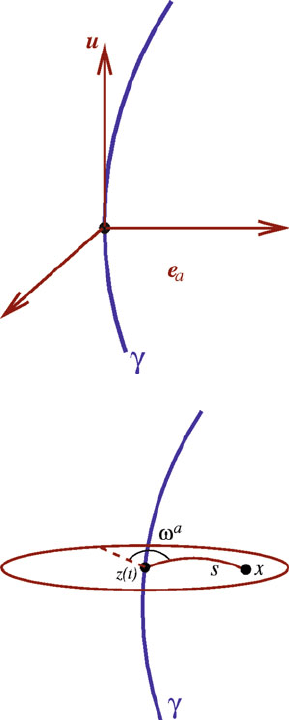
The retarded coordinates .u;x
a
D r˝
a
/ are constructed as follows (LRR
Section 3.3). Once more we select a point x in a neighborhood of the world line,
but this time we locate the unique null geodesic segment ˇ that originates at x and
travels backward in time toward . The new intersection point is labeled x
0
,andu
is the value of the proper-time parameter at this point: x
0
D z. D u/. This defines
the time coordinate u of the point x. The spatial coordinates x
a
are defined exactly
as before, by
x
a
WD e
a
˛
0
.x
0
/
˛
0
.x; x
0
/: (9)
The retarded coordinates come with the condition .x;x
0
/ D 0, which states that
the points x and x
0
D z.u/ are linked by a null geodesic (which travels forward in
time from x
0
to x).
It is useful to introduce r as a measure of light-cone distance between x and the
world line. This is formally defined by r WD
˛
0
.x; x
0
/u
˛
0
.x
0
/, and can be shown to
be an affine parameter on the null geodesic that links x to x
0
(LRR Section 3.3.3).
In addition, we have that r
2
Dı
ab
x
a
x
b
,andr is the usual Euclidean distance as-
sociated with the spatial coordinates x
a
. It is also useful to introduce the direction
cosines ˝
a
WDx
a
=r, which again play the role of a unit radial vector that points
away from the world line.
Each hypersurface u D constant is the future light cone of the point z.u/ on the
world line. Any point x on this light cone is in direct causal contact with z.u/.For
this reason the retarded coordinates give the simplest description of the scalar field
˚ produced by a point charge q moving on the world line. The field satisfies a wave
equation, and the radiation produced by the field essentially realizes the light cones
that are so prominently featured in the construction of the coordinates.
316 E. Poisson
4 Field Equation and Particle Motion
Let me recapitulate the problem that we wish to solve. We have a point particle of
mass m and scalar charge q moving on a world line described by the parametric
relations z
./. The particle creates a scalar field ˚.x/ and this field acts back on
the particle and produces a force F
˛
self
. We wish to determine this self-force.
The scalar field obeys the linear wave equation
˚ D4; (10)
where WD g
˛ˇ
r
˛
r
ˇ
is the wave operator, and
.x/ D q
Z
ı
4
x; z./
d (11)
is the scalar-charge density, expressed as an integral over the world line. The four-
dimensional delta function ı
4
.x; z/ is defined as a scalar quantity; it is normalized
by
R
ı
4
.x; x
0
/
p
gd
4
x D 1.
The particle moves according to
m./a
D q
g
C u
u
˚
; (12)
where a
D Du
=d is the covariant acceleration and ˚
WD r
˚ is the field gra-
dient. The presence of the projector g
Cu
u
on the right-hand side ensures that
the acceleration is orthogonal to the velocity. The field gradient, however, also has a
component in the direction of the world line, and this produces a change in the parti-
cle’s rest mass (LRR Section 5.1.1): dm=d Dqu
˚
. We shall not be concerned
with this effect here. Suffice it to say that the mass is not conserved because the
scalar field can radiate monopole waves, which is impossible for electromagnetic
and gravitational radiation.
The wave equation for ˚ can be integrated, as we shall do in the following sec-
tion, and the solution can be examined near the world line. Not surprisingly, the field
is singular on the world line. This property makes the equation of motion meaning-
less as it stands, and we shall have to make sense of it in the course of our analysis.
5 Retarded Green’s Function
The wave equation for ˚ is solved by means of a Green’s function G.x; x
0
/ that
satisfies
G.x; x
0
/ D4ı
4
.x; x
0
/: (13)
The solution is simply
˚.x/ D
Z
G.x; x
0
/.x
0
/
p
g
0
d
4
x
0
D q
Z
G.x; z/ d; (14)

Constructing the Self-Force 317
and the difficulty of solving the wave equation has been transferred to the difficulty
of computing the Green’s function. We wish to construct the retarded solution to
the wave equation, and this is accomplished by selecting the retarded Green’s func-
tion G
ret
.x; x
0
/ among all the solutions to Green’s equation. (Other choices will be
considered below.) The retarded Green’s function possesses the important property
that it vanishes when the source point x
0
is in the future of the field point x.This
ensures that ˚.x/ depends on the past behavior of the source , but not on its future
behavior.
The retarded Green’s function is known to exist globally as a distribution if the
spacetime is globally hyperbolic. But knowledge of the Green’s function is required
only in the immediate vicinity of the world line, so as to identify the behavior of ˚
there; we shall not be concerned with the behavior of the Green’s function when x
and z./ are widely separated.
In this context the Green’s function can be shown (LRR Section 4.3) to admit a
Hadamard decomposition of the form
G
ret
.x; x
0
/ D U.x;x
0
/ı
future
./ C V.x;x
0
/
future
./; (15)
where .x;x
0
/ is the world function introduced previously, and the two-point func-
tions U.x;x
0
/ and V.x;x
0
/ are smooth when x ! x
0
. The retarded Green’s function
is not smooth in this limit, however, as we can see from the presence of the delta and
theta functions. The first term involves ı
future
./, the restriction of ı./ on the future
light cone of the source point x
0
. The delta function is active when .x;x
0
/ D 0,
and this describes (for fixed x
0
) the future and past light cones of x
0
. We then elim-
inate the past branch of the light cone – for example, by multiplying ı./ by the
step function .t t
0
/ – and this produces ı
future
./. The second term involves
future
./, a step function that is active when <0,thatis,whenx and x
0
are
timelike related; we also restrict the interior of the light cone to the future branch,
so that x is necessarily in the future of x
0
.
The delta term in G
ret
.x; x
0
/ is sometimes called the direct term, and it corre-
sponds to propagation from x
0
to x that takes place directly on the light cone. If the
Green’s function contained a direct term only (as it does in flat spacetime), the field
at x would depend only on the conditions of the source at the corresponding
retarded events x
0
, the intersection between the support of the source and x’s past
light cone. In the case of a point particle this reduces to a single point x
0
z.u/.
The theta term in G
ret
.x; x
0
/, which is sometimes called the tail term, corresponds
to propagation within the light cone; this extra term (which is generically present
in curved spacetime) brings a dependence from events x
0
that lie in the past of the
retarded events. In the case of a point particle, the field at x depends on the particle’s
entire past history, from D1to D u.
There exists an algorithm to calculate U.x;x
0
/ and V.x;x
0
/ in the form of Taylor
expansions in powers of
˛
0
(LRR Section 4.3.2). It returns
U.x;x
0
/ D 1 C
1
12
R
˛
0
ˇ
0
˛
0
ˇ
0
C (16)
318 E. Poisson
and
V.x;x
0
/ D
1
12
R.x
0
/ C; (17)
where R
˛
0
ˇ
0
is the Ricci tensor at x
0
,andR.x
0
/ the Ricci scalar at x
0
. In Ricci-flat
spacetimes the expansions of U 1 and V both begin at the fourth order in
˛
0
.
6 Alternate Green’s Function
The advanced Green’s function is given by (LRR Section 4.3)
G
adv
.x; x
0
/ D U.x;x
0
/ı
past
./ C V.x;x
0
/
past
./; (18)
in terms of the same two-point functions U.x;x
0
/ and V.x;x
0
/ that appear within
the retarded Green’s function. The difference is that the light cones are now
restricted to the past branch, so that G
adv
.x; x
0
/ vanishes when x
0
is in the past
of x. A solution to the wave equation constructed with the advanced Green’s func-
tion would display anti-causal behavior: it would depend on the future history of
the source.
Another useful choice of Green’s function is the Detweiler–Whiting singular
Green’s function defined by (LRR Section 4.3.5)
G
S
.x; x
0
/ D
1
2
U.x;x
0
/ı./
1
2
V.x;x
0
/./: (19)
Here the delta and theta functions are no longer restricted: both future and past
branches contribute to the Green’s function. In fact, the argument of the step func-
tion is now C, and this indicates that the second term is active when x and x
0
are
spacelike related. For fixed x
0
, the singular Green’s function is nonzero when x is
either on, or outside, the (past and future) light cone of x
0
. Unlike the retarded and
advanced Green’s functions, G
S
.x; x
0
/ is not known to exist globally as a distribu-
tion (even for globally hyperbolic spacetimes); its local existence is not in doubt,
however, and this suffices for our purposes.
All three Green’s functions satisfy the same wave equation, G D4ı
4
,and
all three give rise to fields ˚.x/ that diverge on the particle’s world line. A use-
ful combination of Green’s functions is the Detweiler–Whiting regular two-point
function
G
R
.x; x
0
/ D G
ret
.x; x
0
/ G
S
.x; x
0
/; (20)
which satisfies the homogeneous wave equation G
R
.x; x
0
/ D 0. This two-point
function gives rise to a field
˚
R
D ˚
ret
˚
S
(21)
that also satisfies the homogeneous wave equation, ˚
R
D 0. This field is the
difference between two singular fields, and since ˚
ret
and ˚
S
are equally singular
Constructing the Self-Force 319
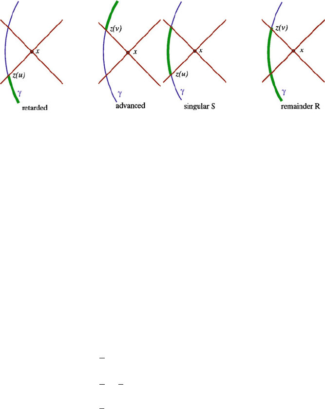
Fig. 5 Solutions to the wave equation. The retarded field is sourced by the past history of the
point particle, up to the retarded position z.u/. The advanced field is sourced by the future history,
starting from the advanced position z.v/. The singular field is sourced by the world-line segment
that lies on and outside the light cone of the field-point x, starting from the retarded position z.u/
and ending at the advanced position z.v/. Finally, the regular field is sourced by the history of the
particle up to the advanced position z.v/
near the world line, we find that the regular remainder field ˚
R
stays bounded when
x ! z./. And what’s more, the regular field is smooth, in the sense that it and any
number of its derivatives possess a well-defined limit when x ! z. / (Fig.5).
7 Fields Near the World Line
Using the ingredients presented in the preceding sections it is possible to show (LRR
Sections 5.1.3–5.1.5) that close to the world line, the retarded, singular, and regular
fields are given by
˚
ret
D
q
r
C q
Z
u
1
V.x;z/d C O.r
2
/; (22a)
˚
S
D
q
r
1
3
q Pa
a
x
a
C O.r
2
/; (22b)
˚
R
D
1
3
q Pa
a
x
a
C q
Z
u
1
V.x;z/d C O.r
2
/; (22c)
in the retarded coordinates .u;x
a
Dr˝
a
/. These expressions involve the re-
tarded distance r from x to z.u/ and the frame component Pa
a
.u/ WD Pa
e
a
of
Pa
WDDa
=d , the proper-time derivative of the acceleration vector. They
involve also an integration over the past history of the particle. These expressions
are valid for Ricci-flat spacetimes. We observe that the retarded and singular fields
both diverge as q=r as we approach the world line, but that the regular remainder
˚
R
is free of singularities.
320 E. Poisson
In the Fermi coordinates .t; x
a
D s!
a
/ we have the more complicated
expressions:
˚
ret
D
q
s
1
2
qa
a
!
a
C qs
1
8
Pa
0
C
1
3
Pa
a
!
a
1
6
R
0a0b
!
a
!
b
Cq
Z
t
1
V.x;z/d C O.s
2
/; (23a)
˚
S
D
q
s
1
2
qa
a
!
a
C qs
1
8
Pa
0
1
6
R
0a0b
!
a
!
b
C O.s
2
/; (23b)
˚
R
D
1
3
q Pa
a
x
a
C q
Z
t
1
V.x;z/d C O.s
2
/: (23c)
They involve the spatial distance s between x and z.t/, the frame components of
the acceleration vector and its proper-time derivative, the frame components of the
Riemann tensor, and the integration over the past history of the particle. Once more
we see that the retarded and singular fields diverge in the limit s !0, but that the
regular field is free of singularities. (The singular nature of ˚
S
is also observed
in a term such as
1
2
qa
a
!
a
that stays bounded when s ! 0, but is directionally
ambiguous on the world line.)
From these equations we may calculate the spatial derivatives of the singular and
regular fields. We obtain
r
a
˚
S
D
q
s
2
!
a
q
2s
ı
b
a
!
b
!
a
a
b
C
q
8
Pa
0
!
a
C
q
6
R
0b0c
!
a
!
b
!
c
q
3
R
0a0b
!
b
C O.s/; (24a)
r
a
˚
R
D
1
3
q Pa
a
C q
Z
t
1
r
a
V.x;z/d C O.s/: (24b)
As expected, the gradient of the singular field diverges as q=s
2
, but the gradient of
the regular field is free of singularities. The gradient of the retarded field is r
a
˚
ret
D
r
a
˚
S
Cr
a
˚
R
.
We notice that many terms in r
a
˚
S
are proportional to an odd number of radial
vectors !
a
; all such terms vanish when we average the field gradient over a spherical
surface of constant s. This averaging leaves behind
˝
r
a
˚
S
˛
D
q
3s
a
a
C O.s/; (25)
which is still singular. To obtain this result we made use of the identity h!
b
!
a
iD
1
3
ı
b
a
. Notice that because r
a
˚
R
is smooth at s D 0, an averaging simply returns the
same expression: hr
a
˚
R
iDr
a
˚
R
.