Biringen S., Chow C.-Y. An Introduction to Computational Fluid Mechanics by Example

Подождите немного. Документ загружается.

142 INVISCID FLUID FLOWS

1.4 1.5 1.6 1.7 1.8 1.9 2 2.1

−20

100

Velocity [cm/s]

1.4 1.5 1.6 1.7 1.8 1.9 2 2.1

100

110

time [s]

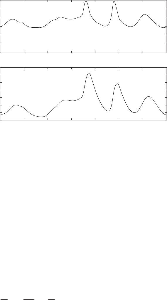
z = 22 cm

(c)

Pressure [mmHg]

FIGURE 2.13.8 (continued).

We should also note that although the signal propagating in the elastic tube

converges to a quasi-steady periodic state, the initial transients in the solution can

have very steep fronts necessitating the implementation of artiﬁcial dissipation.

As we explained above, smoothing irregular and sharp signals with such mea-

sures is not uncommon in the applications of computational models to ﬂuid ﬂow

problems, as the governing equations are nonlinear and would interact through

the advection terms (e.g., V (∂V/∂z)), resulting in energy accumulating in higher

harmonics, which are not resolved by the given ﬁnite difference mesh. If the phys-

ical dissipation is not sufﬁcient to dampen out these growing numerical errors,

or if the integration scheme, i.e., the ﬁnite difference formula is not sufﬁciently

dissipative, then one would have to explicitly add an artiﬁcial dissipation term

to the ﬁnite difference equations. For ﬁnite difference formulas that are second-

order accurate in space, the addition of a fourth-order artiﬁcial dissipation term

is generally sufﬁcient, and will not decrease the formal accuracy of the method if

the coefﬁcient ω is small. In this problem, we add (2.13.12) to the right-hand side

of the ﬁnite difference equations, which, for the velocity component of (2.13.35),

can be written as

D =−

(z)

∂

∂z

=−

i+2

−4V

i+1

+6V

−4V

i−1

i−2

) (2.13.44)

APPENDIX 143

The negative sign ensures that positive dissipation is produced. The artiﬁcial

dissipation coefﬁcient was set to μ

= 0.04, so that the effect of this parameter

is not signiﬁcant on solution accuracy.

Problem 2.15 Construct a MATLAB code to solve the system of equations

(2.13.35)–(2.13.37) using the MacCormack explicit method, with the information

provided in this section to investigate the inﬂuence of the following parameters

on the solution: (a) double the frequency of the forcing (proximal boundary

condition for pressure); (b) halve the frequency of the forcing; (c) double the

amplitude of the forcing; (d) halve the amplitude of the forcing. For all these

cases, plot pressure and velocity as a function of time at speciﬁed locations along

the vessel.

A formula for turbulent ﬂow for the friction function f is given by Anliker

and Rockwell (1971). This expression is written as

turbulent

=−0.1360





1/4

|V |

7/4

5/8

sgn V (2.13.45)

Use this expression instead of the laminar formula (2.13.41). Compare the ampli-

tude and frequency responses of the pressure and velocity at several locations

along the axis of the vessel.

In all these calculations, it is important to run the code at least three periods

of the forcing frequency. For example, if the period is 0.7 s, then the total time

should be about 2.1–3.8 s. It is also important to note that if the solutions become

unstable for some combination of these parameters, it is generally due to the steep

front of the initial transients that produce large-amplitude higher harmonics in the

pressure. These oscillations can be controlled by increasing the artiﬁcial viscosity

coefﬁcient or by reducing the time step.

APPENDIX

TABLE 2.A.1 Output of Program 2.1

I R(I) PHI(I) EXPHI(I) U(I) EXU(I)

1.0000e+00 1.1000e+00 −9.5430e−01 −9.5644e−01 −1.8220e+01 −1.8188e+01

2.0000e+00 1.2000e+00 −2.6440e+00 −2.6477e+00 −1.5702e+01 −1.5680e+01

3.0000e+00 1.3000e+00 −4.0948e+00 −4.0997e+00 −1.3407e+01 −1.3392e+01

0000e+00 1.4000e+00 −5.3254e+00 −5.3313e+00 −1.1274e+01 −1.1263e+01

5.0000e+00 1.5000e+00 −6.3496e+00 −6.3562e+00 −9.2579e+00 −9.2500e+00

6.0000e+00 1.6000e+00 −7.1770e+00 −7.1841e+00 −7.3253e+00 −7.3200e+00

7.0000e+

00 1.7000e+00 −7.8147e+00 −7.8221e+00 −5.4511e+00 −5.4476e+00

8.0000e+00 1.8000e+00 −8.2672e+00 −8.2749e+00 −3.6153e+00 −3.6133e+00

9.0000e+00 1.9000e+00 −8.5377e+00 −8.5455e+00 −1.8025e+00 −1.8016e+00

(continues)

144 INVISCID FLUID FLOWS

TABLE 2.A.1 (continued)

I R(I) PHI(I) EXPHI(I) U(I) EXU(I)

1.0000e+01 2.0000e+00 −8.6277e+00 −8.6355e+00 −5.2788e−05 1.5987e−14

1.1000e+01 2.1000e+00 −8.5377e+00 −8.5455e+00 1.8020e+00 1.8014e+00

1.2000e+01 2.2000e+00 −8.2673e+00 −8.2750e+00 3.6120e+00 3.6109e+00

1.3000e+01 2.3000e+00 −7.

8153e+00 −7.8228e+00 5.4368e+00 5.4352e+00

1.4000e+01 2.4000e+00 −7.1800e+00 −7.1872e+00 7.2819e+00 7.2800e+00

1.5000e+01 2.5000e+00 −6.3590e+00 −6.3660e+00 9.1521e+00 9.1500e+00

1.6000e+01 2.6000e+00 −5.3495e+00 −5.3563e+00 1.1052e+01 1.

1049e+01

1.7000e+01 2.7000e+00 −4.1486e+00 −4.1550e+00 1.2984e+01 1.2981e+01

1.8000e+01 2.8000e+00 −2.7528e+00 −2.7589e+00 1.4951e+01 1.4949e+01

1.9000e+01 2.9000e+00 −1.1584e+00 −1.1641e+00 1.6957e+01 1.6954e+01

2.0000e+01 3.0000e+00 6.3853e

−01 6.3331e−01 1.9003e+01 1.9000e+01

2.1000e+01 3.1000e+00 2.6421e+00 2.6373e+00 2.1091e+01 2.1088e+01

2.2000e+01 3.2000e+00 4.8567e+00 4.8524e+00 2.3223e+01 2.3220e+01

2.3000e+01 3.3000e+00 7.2867e+00 7.2829e+00 2.5400e+01 2.5397e+01

2.4000e+01 3.4000e+00 9.9367e+

00 9.9334e+00 2.7624e+01 2.7621e+01

2.5000e+01 3.5000e+00 1.2812e+01 1.2809e+01 2.9896e+01 2.9893e+01

2.6000e+01 3.6000e+00 1.5916e+01 1.5914e+01 3.2216e+01 3.2213e+01

2.7000e+01 3.7000e+00 1.9255e+01 1.9253e+01 3.4586e+01 3.4584e+01

2.8000e+01 3.8000e+00 2.2833e+01 2

.2832e+01 3.7007e+01 3.7004e+01

2.9000e+01 3.9000e+00 2.6656e+01 2.6656e+01 3.9479e+01 3.9476e+01

VISCOUS FLUID FLOWS

The viscous effects ignored in the previous chapter are examined in this chapter.

The governing equations for viscous ﬂows are ﬁrst summarized in Section 3.1. The

numerical techniques, devised previously for solving ordinary initial-value and

boundary-value problems, are then used or modiﬁed to be used in the next two

sections to study a velocity boundary layer and a thermal boundary layer. In

Section 3.4, an open-channel ﬂow problem is solved utilizing a numerical method

constructed in Section 2.8 for solving elliptic partial differential equations.

There are two different approaches in solving parabolic equations. The explicit

methods and their computational stabilities are discussed in Section 3.5, with an

example given on the unsteady ﬂow caused by a suddenly accelerated plane wall.

The computationally stable implicit methods are introduced in Section 3.6. The

illustrative example used there is the starting ﬂow in a channel caused by the

application of a constant pressure gradient.

Section 3.7 deals with Stokes ﬂows, which are governed by a biharmonic

equation. Such an equation is solved by ﬁrst rewriting it in the form of two

coupled elliptic equations and then by applying twice an appropriate iterative

method derived in Section 2.8. This numerical scheme is used to solve for the

cavity ﬂow caused by a moving surface. The last section, Section 3.8, concerns

the linear stability of viscous ﬂows where we also introduce the basic ideas of

pseudo-spectral methods.

3.1 GOVERNING EQUATIONS FOR VISCOUS FLOWS

Before solving viscous ﬂow problems, the equations governing the unsteady

motion of a viscous compressible ﬂuid having variable physical properties are

summarized. Derivation of these equations can be found in many texts on ﬂuid

145

An Introduction to Computational Fluid Mechanics by Example Sedat Biringen and Chuen-Yen Chow

146 VISCOUS FLUID FLOWS

dynamics, for example, in Schlichting (1968). The equations are expressed here

in vector notation. Their speciﬁc forms in Cartesian, cylindrical, and spherical

coordinates are shown in the book by Hughes and Gaylord (1964).

No matter whether the ﬂuid is viscous or inviscid, the continuity equation

(2.11.11) remains in the same form, so that

∂ρ

∂t

+∇ ·(ρV) = 0 (3.1.1)

However, viscous forces appear in a real ﬂuid, as discussed in Section 2.1. The

equation of motion, constructed by adding to Euler’s equation (2.1.5) the forces

per unit volume caused by viscosity, is of the form

=−∇p −∇ × [μ(∇ × V)] + ∇[(2μ +λ)∇ · V] (3.1.2)

The operator on the left side, deﬁned previously in (2.1.6), is the substantial

derivative. μ is the coefﬁcient of viscosity, and λ is the second coefﬁcient of

viscosity of the ﬂuid; both are functions of temperature. For a monatomic gas

λ =−

μ. Equation (3.1.2) is generally referred to as the Navier-Stokes equation.

The addition of viscous forces increases the order of the differential equation by

one. The extra constant of integration to appear in the solution is determined from

the additional boundary condition required for a viscous ﬂuid that the velocity

component tangent to a stationary rigid surface must also be zero. The boundary

condition for an inviscid ﬂuid is that the component normal to such a surface

vanishes.

The energy equation may be written in several alternative forms. The following

form is often used for an ideal gas in terms of speciﬁc enthalpy h (= c

T):

+∇ ·(k∇T ) + (3.1.3)

in which c

and k are, respectively, the constant-pressure speciﬁc heat and the

thermal conductivity of the gas, T is the absolute temperature, and  is the

dissipation function deﬁned in Cartesian coordinates as

 = 2μ





∂u

∂x





∂v

∂y





∂w

∂z





+μ



∂u

∂y

∂v

∂x



+μ



∂v

∂z

∂w

∂y



+μ



∂w

∂x

∂u

∂z



+λ(∇ · V)

(3.1.4)

It represents the time rate at which energy of the ordered ﬂuid motion per unit

volume is dissipated into heat through the action of viscosity.

Finally, the equation of state for an ideal gas is

p = ρRT (3.1.5)

where R is the gas constant.

SELF-SIMILAR LAMINAR BOUNDARY-LAYER FLOWS 147

We now have six scalar equations, (3.1.1) to (3.1.3) and (3.1.5), with (3.1.2)

written in component form, which form a complete set of equations for the six

unknowns ρ, p, T , u, v,andw. To ﬁnd solutions to this system is extremely

difﬁcult because not only are the equations nonlinear, but also the unknowns are

related in such a way that all six equations must be solved simultaneously.

Great simpliﬁcations are obtained by assuming that the ﬂuid is incompressible

and the temperature variation is not too large so that ﬂuid properties are constant.

In this case ρ becomes a constant, the equation of state is not needed, and the

energy equation is uncoupled from the continuity equation and the equation of

motion. The latter two are simpliﬁed in Cartesian coordinates to

∇ · V = 0 (3.1.6)

=−∇p + μ∇

V (3.1.7)

The procedure for solving the problem is ﬁrst to obtain p and V from simultane-

ous equations (3.1.6) and (3.1.7), and then to ﬁnd T after substituting the result

into the simpliﬁed version of (3.1.3).

It is still possible to introduce the stream function deﬁned in Section 2.1; the

velocity potential can no longer be used because the ﬂow is generally rotational

in the presence of rotational viscous forces.

3.2 SELF-SIMILAR LAMINAR BOUNDARY-LAYER FLOWS

A very important example that exhibits self-similarity is the high Reynolds num-

ber ﬂow past a streamline body discussed in Section 2.1. In this case effects of

viscosity and conductivity are conﬁned within a thin boundary layer next to the

body surface.

The governing equations for boundary-layer ﬂows are deduced from Navier-

Stokes equations under the assumption that the boundary-layer thickness δ is

small compared with the characteristic length L of the body. Considering a thin,

two-dimensional boundary layer around a body having its surface parallel to the

x axis and normal to the y-axis, Kuethe and Chow (1998, Appendix B), using an

order-of-magnitude analysis, found that v  u and ∂/∂x  ∂/∂y when operating

on either velocity or temperature. If the x component of the equation of motion is

of order unity, then the y component is of order δ/L. When the latter is ignored

completely, with ∂p/∂y approximated by zero, the resulting Navier-Stokes and

energy equations are, respectively,



∂u

∂t

∂u

∂x

∂u

∂y



=−

∂p

∂x

∂

∂y



∂u

∂y



(3.2.1)

ρc



∂T

∂t

∂T

∂x

∂T

∂y



∂p

∂t

∂p

∂x

∂

∂y



∂T

∂y



+μ



∂u

∂y



(3.2.2)

148 VISCOUS FLUID FLOWS

They are called the boundary-layer equations for two-dimensional compressible

ﬂow. These, together with the continuity equation (3.1.1) and the equation of

state (3.1.5), form a system of four scalar equations for the four unknowns ρ,

T, u,andv. The pressure p in a thin boundary layer is no longer treated as

an unknown. Instead, it is considered to be constant across the boundary layer,

while its x dependence is obtained by solving the problem of an inviscid ﬂow

past the same body. The previously mentioned approximations form the basis of

Prandtl’s boundary-layer theory.

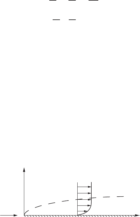
If we consider the simple problem of a semi-inﬁnite ﬂat plate aligned with a

uniform ﬂow of constant speed U and of constant physical properties, including

density ρ, as sketched in Fig. 3.2.1, the governing equations for a steady ﬂow

are further simpliﬁed to

∂u

∂x

∂u

∂y

= ν

∂

∂y

(3.2.3)

∂u

∂x

∂v

∂y

= 0 (3.2.4)

where ν = μ/ρ is the kinematic viscosity of the ﬂuid. These two equations are

sufﬁcient for computing the velocity ﬁeld. The use of the decoupled energy

equation will be demonstrated in Section 3.3. This formulation closely describes

the thin laminar boundary layer on the surface of a two-dimensional streamlined

body that moves in an incompressible ﬂuid, or in a compressible ﬂuid but at a

speed much slower than the speed of sound.

At any ﬁxed x on the plate, three boundary conditions are needed, two for

the ﬁrst equation and one for the second. They are the no-slip condition at the

surface and the condition of uniform ﬂow at inﬁnity; that is,

u = v = 0aty = 0 (3.2.5)

u → U as y →∞ (3.2.6)

Finding a solution to the system consisting of (3.2.3) to (3.2.6) is called the Bla-

sius problem (Blasius, 1908). In terms of stream function ψ deﬁned in (2.1.14),

y = δ(x)

FIGURE 3.2.1 Boundary layer on a ﬂat plate.

SELF-SIMILAR LAMINAR BOUNDARY-LAYER FLOWS 149

that is, u = ∂ψ/∂y and v =−∂ψ/∂x, (3.2.4) is satisﬁed automatically and (3.2.3)

becomes

∂ψ

∂y

∂

∂x∂y

−

∂ψ

∂x

∂

∂y

= ν

∂

∂y

(3.2.7)

Experiments show that by stretching the vertical coordinate according to the

law y/

√

x, the dimensionless velocity proﬁles u/U measured in a laminar bound-

ary layer at different distances x from the leading edge collapse into one. In other

words, these velocity proﬁles are similar to one another, and the boundary layer

ﬂowissaidtobeself-similar. This evidence suggests a great simpliﬁcation for our

mathematical analysis of the Blasius problem. If the independent variables x and

y were combined according to the stretching law just mentioned to form a new

single independent variable η, we would expect that the governing partial differ-

ential equation (3.2.7) could be transformed into an ordinary differential equation

and that the boundary conditions (3.2.5) and (3.2.6) would contain neither x nor

y explicitly.

Let us try the following transformations, in which η is nondimensionalized

and f is a dimensionless function:

η = y



νx



1/2

(3.2.8)

ψ = (νUx)

1/2

f (η) (3.2.9)

In terms of the new variables, and with a prime denoting differentiation with

respect to η, the velocity components become

u = Uf



(3.2.10)

v =



νU



1/2

(ηf



−f ) (3.2.11)

and the governing equation becomes





= 0 (3.2.12)

with boundary conditions

f = f



= 0atη = 0 (3.2.13)



→ 1asη →∞ (3.2.14)

Sure enough we have reduced our problem to solving an ordinary differential

equation, although it is still a nonlinear equation. η is called the similarity vari-

able, and the solution to the transformed system is called the similarity solution

of the original formulation.

It should be pointed out that the transformations (3.2.8) and (3.2.9) are not

valid at the leading edge where x = 0, and that x (or y) must appear on the

150 VISCOUS FLUID FLOWS

right-hand side of (3.2.9) if u/U is to be a function of η alone. Actually, these

two transformations would also be derived if we started with the general form that

η = Ax

y and ψ = Bx

f (η), and if we then required that after transformation x

and y could not appear explicitly.

The solution of (3.2.12) satisfying accompanying boundary conditions was

obtained by Blasius (1908) in the form of a power series expansion about η = 0

and an asymptotic expansion for η →∞, the two being matched at an interme-

diate point. Here we will ﬁnd the solution using a numerical approach.

If f , f



,andf



are all known at a certain dimensionless height η

, the fourth-

order Runge-Kutta method may be utilized to ﬁnd the solution η

i+1

= η

+h and

at stations thereafter step by step. To prepare for using the method, the third-order

equation (3.2.12) is ﬁrst written as three ﬁrst-order simultaneous equations:

dη

= p,

dη

= q,

dη

=−

fq (3.2.15)

Then the Runge-Kutta formulas (1.1.9) are applied to each of them to get



= hp



= hq



=−



= h(p



)



= h(q



)



=−

h( f



)(q



)



= h(p



)



= h(q



)



=−

h( f



)(q



)



= h(p

+

)



= h(q

+

)



=−

h( f

+

)(q

+

)

(3.2.16)

Finally, the values of f, f



,andf



are computed at η

i+1

by analogy with (1.1.8):

i+1

= f

(

+2

+

)

i+1

= p

(

+2

+

)

i+1

= q

(

+2

+

)

(3.2.17)

However, numerical integration of (3.2.15) cannot be started at η = 0 because

q (i.e., f



) is not known there. Boundary conditions (3.2.13) and (3.2.14) provide

SELF-SIMILAR LAMINAR BOUNDARY-LAYER FLOWS 151

only two of the three values, f and p (or f



), that are required at η = 0, but

provide another value of p at inﬁnity. If the problem is to be solved by the

Runge-Kutta method, it may be combined with the half-interval method already

introduced in Section 1.5, as follows.

First, the boundary condition (3.2.14) at inﬁnity is not convenient for pro-

gramming, since every value speciﬁed or computed in a program must be ﬁnite.

Instead of extending to inﬁnity, we limit our range of numerical integration up

to a reasonably large height η

max

and approximate (3.2.14) by

1 − p ≤  at η = η

max

(3.2.18)

where  represents a positive value much less than unity whose magnitude

controls the accuracy of the solution.  must be positive because p is the dimen-

sionless parallel velocity component in the boundary layer that approaches the

free-stream value of 1 from below.

At the beginning of our numerical computation a value q

is arbitrarily guessed

and a positive increment 

is picked. By letting f = p = 0andq = q

η = 0, (3.2.15) are integrated using Runge-Kutta formulas until η reaches η

max

The last value of p so computed is designated p

max

and is represented by the

leftmost point on the q

versus p

max

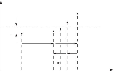
plot of Fig. 3.2.2. If the ordinate of this point

is below the value 1, as shown, we replace the starting value q

of q by q

+

and repeat the numerical integration from η = 0. The process would be repeated

again if the same ﬁnal situation were encountered at η

max

. Suppose at the end of

the third time a point above the dashed horizontal line of unit height is obtained;

we know that the starting value of q is now too large. To reverse the direction, we

let 

=−

/2 and then replace q

by q

+

. Repeat with this negative

value of 

until the data point in Fig. 3.2.2 comes below the horizontal

dashed line. Then we reverse the direction again by letting 

=−

/2and

Error

= f''(0)

max

FIGURE 3.2.2 Half-interval method for the Blasius problem.