Biringen S., Chow C.-Y. An Introduction to Computational Fluid Mechanics by Example

Подождите немного. Документ загружается.

122 INVISCID FLUID FLOWS

and a

are computed immediately by adding and subtracting the above

equations. Thus,

) +

γ −1

−a

) (2.12.6)

γ −1

−u

) +

) (2.12.7)

Although the exact shape of the characteristics cannot be determined unless u

and a are both known in the region below point C , the solution may be com-

puted approximately if the distance between points A and B is small. Under this

condition the curved characteristics can be treated as two straight lines of slopes

and u

−a

, respectively, and the conditions at point C , which is the

intersection of these two straight lines, are described approximately by (2.12.6)

and (2.12.7).

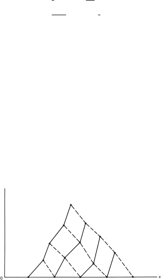
Thus, when a row of points is selected at small distances apart on the x axis

at t = 0, the solution can be computed step by step at later times by constructing

a network using the local slopes of the characteristics, shown in Fig. 2.12.2. This

method, however, is not practical for machine calculation, because the locations

of data points in the network are not known a priori. Many ﬁnite-difference

techniques have been developed for solving the same problem on a predeter-

mined rectangular mesh. The one chosen to be used here, suggested by Courant,

Isaacson, and Rees (1952), is convenient for programming and yet is physically

interpretable.

Let us adopt a grid system, exactly the same as that sketched in Fig. 2.10.1, for

numerical solution of the simultaneous nonlinear equations (2.12.4) and (2.12.5).

Suppose u and a have already been computed at all grid points on time level

; we now proceed to ﬁnd the conditions at the grid points on the next time

level t

j+1

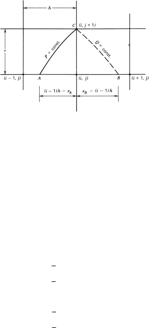
, for example, at point C ,or(i, j + 1), as shown in Fig. 2.12.3. If the

FIGURE 2.12.2 Characteristic network.

PROPAGATION OF A FINITE-AMPLITUDE WAVE: FORMATION OF A SHOCK 123

FIGURE 2.12.3 Finite-difference scheme for a rectangular mesh.

characteristics through this point intersect with the back horizontal grid line at

points A and B, respectively, then, according to the method of characteristics

described in Fig. 2.12.1, the condition at C is determined approximately from

those at A and B by using formulas (2.12.6) and (2.12.7). The location and

condition at points A and B are to be interpolated from the known information

at grid points on that same time level.

Treating the characteristics as straight lines and approximating their slopes by

i, j

and u

i, j

−a

i, j

respectively, we ﬁnd, from Fig. 2.12.3,

= (i −1)h − τ

)

i, j

(2.12.8)

= (i −1)h − τ

)

i, j

−a

i, j

(2.12.9)

After points A and B have been located, linear interpolations are then used to

ﬁnd u

and a

within the interval between x

i−1

and x

. Thus,

= u

i, j

)

i, j

i−1, j

−u

i, j

(2.12.10)

= a

i, j

)

i, j

i−1, j

−a

i, j

(2.12.11)

Similarly, at B,

= u

i, j

−

)

i, j

−a

i, j

i+1, j

−u

i, j

(2.12.12)

= a

i, j

−

)

i, j

−a

i, j

)(a

i+1, j

−a

i, j

(2.12.13)

124 INVISCID FLUID FLOWS

and a

or, in fact, u

i, j +1

and a

i, j +1

are computed immediately following the

substitution of (2.12.10) to (2.12.13) into (2.12.6) and (2.12.7).

Detailed analysis of this numerical method has been made by Courant et al.

for a more general system of equations. The result is accurate to the ﬁrst order

of h. For computational stability it requires that the ratio τ/h be so chosen that

the numerical domain of dependence of any point in the mesh is not less than

the physical domain of dependence determined by the characteristics. In other

words, the stability condition is that both

u +a

≤ 1and

u −a

≤ 1 (2.12.14)

are satisﬁed everywhere in the domain of computation.

An improved numerical scheme with second-order accuracy was outlined by

Hartree (1958). In his method the curved characteristics through C are approx-

imated by two straight lines whose slopes are, respectively, the average of the

values at C and A and the average of those at C and B instead of the values at

(i, j ). The improved accuracy is paid for by the increased effort in computing the

conditions at points A and B by iteration. In the following example the simpler

method of Courant et al. will be used for the purpose of illustration.

A 2-m-long tube is considered whose left end is closed and right end is open,

similar to the tube shown in Fig. 2.11.1. The length of the tube is again divided

into 0.02-m intervals, resulting in 101 vertical grid lines for the numerical work.

Let a

be the speed of sound in the tube in an undisturbed state. At t = 0a

rightward-propagating wavelet of 1-m wavelength is produced in the left half

of the tube. To exaggerate the effect of ﬁnite amplitude and to show an easily

recognized distortion in wave shape, we assume that the initial amplitude of the

wavelet is a

/2 and that its initial shape is described by a set of broken straight

lines deﬁned by

i,1

⎧

⎪

⎨

⎪

⎩

i − 1

for 1 ≤ i ≤ 13

26 − i

for 13 < i ≤ 39

i −51

for 39 < i ≤ 51

0elsewhere

The initial condition for a is determined by that for u through

a = a

γ −1

u (2.12.15)

which relates the local speed of sound to the local particle velocity (same sign

as x) in an isentropic wave. The negative sign is to be taken only if the wave is

traveling in the negative x direction. The derivation of (2.12.15) can be found in

Section 3.9 of Liepmann and Roshko (1957) and therefore is not repeated here.

PROPAGATION OF A FINITE-AMPLITUDE WAVE: FORMATION OF A SHOCK 125

The boundary conditions at the ends can be derived with the help of Fig. 2.12.3.

At the left end of the tube where i = 1, only one backward characteristic can be

drawn through a grid point along which Q = constant. Combining this with the

condition that particle velocity vanishes at a closed end gives

1, j +1

= 0 (2.12.16)

1, j +1

= a

−

γ −1

(2.12.17)

where u

and a

are computed for i = 1 from (2.12.12) and (2.12.13). At a

grid point at the right end of the tube open to the atmosphere, the density and

therefore the sonic speed is the same as that outside. Furthermore, through such a

point there is only one backward characteristic along which P = constant. Thus,

the boundary conditions there are

m, j +1

= u

γ −1

−a

) (2.12.18)

m, j +1

= a

(2.12.19)

where m is the maximum value of i and u

, a

are computed from (2.12.10) and

(2.12.11) for i = m.

The variables in Program 2.9 are named according to their original form. For

example,

UA, UB, AA,andAB represent, respectively, u

, u

, a

,anda

.Weuse

AMPLTD for the initial amplitude of the velocity distribution, RATIO for τ /h,and

COEFF for (γ − 1)/2.

γ is chosen to be 1.4 for air at sea level. For the ﬁxed value of h = 0.02 m,

the size of time steps is determined from the stability condition (2.12.14). It

involves u and a, which are both unknown before the problem is solved. In the

program a trial value τ = 0.5h/a

is used. Before computing the solution at a

grid point, we check (2.12.14) and discontinue the computation whenever this

condition is violated. The result shows that this trial value is satisfactory for the

present problem at all grid points.

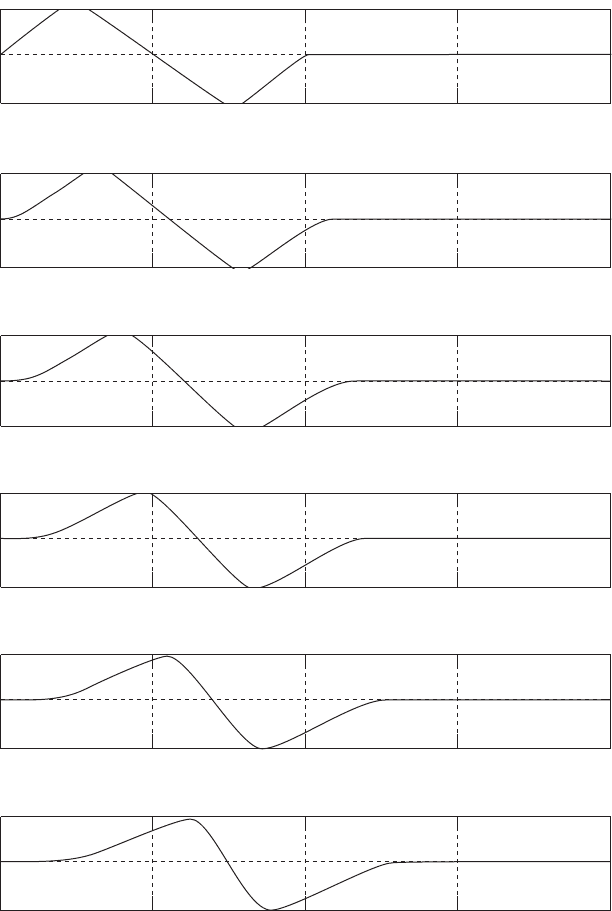
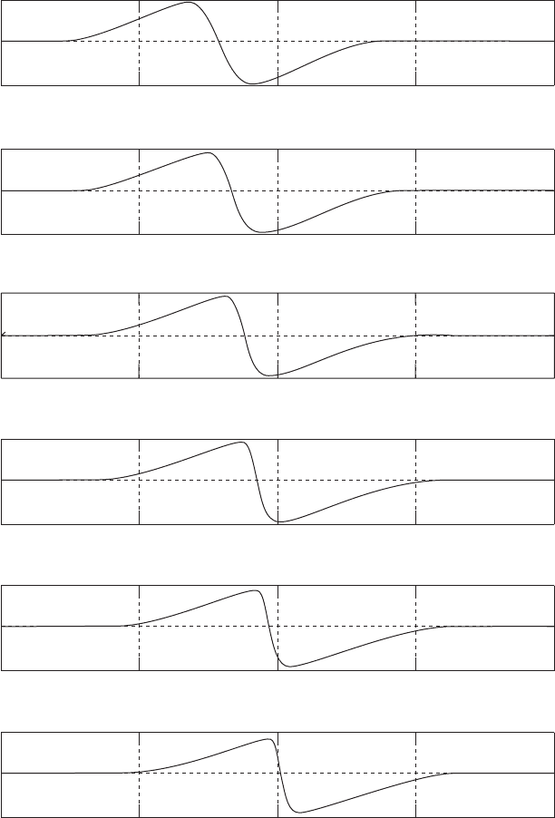
The output of Program 2.9 displays the velocity distributions at increasing

time steps (Time Series 2). It is now examined to ﬁnd the effects of keeping the

nonlinear terms in the governing equations.

In the central part of the wave ∂u/∂x is negative; that is, the right-moving

velocity of a gas particle is faster than that of a particle ahead of it. Thus, in this

region gas particles are catching up with those ahead; this is called a compression

region. The time sequence plots show that the width of this region decreases with

time, so that the wave proﬁle is steepening in the central portion. On the other

hand, in the leading and trailing parts of the wave where ∂u/∂x is positive, gas

particles ahead are moving faster than those behind. In each of these expansion

regions the width increases and the proﬁle ﬂattens with increasing time.

As the wave propagates its proﬁle is no longer antisymmetric about the node.

The left portion, within which u is positive, becomes shorter than that on the

right portion, within which u is negative, while the total length of the wave is

126 INVISCID FLUID FLOWS

0 0.5 1 1.5 2

−150

150

Time = 0*TAU = 0 seconds

0 0.5 1 1.5 2

−150

150

Time = 5*TAU = 0.00014706 seconds

0.5 1 1.5 2

−150

150

Time = 10*TAU = 0.00029412 seconds

0 0.5 1 1.5 2

−150

150

Time = 15*TAU = 0.00044118 seconds

0 0.5 1 1.5 2

−150

150

Time = 20*TAU = 0.00058824 seconds

0 0.5 1 1.5 2

−150

150

Time = 25*TAU = 0.00073529 seconds

Time Series 2 Plate 1.

PROPAGATION OF A FINITE-AMPLITUDE WAVE: FORMATION OF A SHOCK 127

0 0.5 1 1.5 2

−150

150

Time = 30*tau = 0.00088235 seconds

0 0.5 1 1.5 2

−150

150

Time = 35*tau = 0.0010294 seconds

0.5 1 1.5 2

−150

150

Time = 40*tau = 0.0011765 seconds

0 0.5 1 1.5 2

−150

150

Time = 45*tau = 0.0013235 seconds

0 0.5 1 1.5 2

−150

150

Time = 50*tau = 0.0014706 seconds

0 0.5 1 1.5 2

−150

150

Time = 55*tau = 0.0016176 seconds

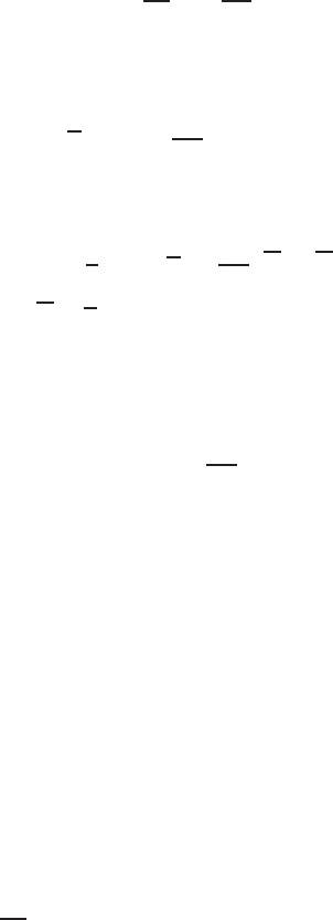
Time Series 2 Plate 2.

128 INVISCID FLUID FLOWS

kept constant. In addition, the amplitude of the wave on the left side of the node

diminishes faster in time than that on the right.

When t = 40τ, the wave proﬁle in the compression region becomes almost

a vertical line. In other words, at this time a drastic change in u can be found

across a very short distance. This is, in fact, a shock wave.

Actually, as explained by Liepmann and Roshko (1957, Section 3.10), before

this situation is reached, the velocity gradient becomes so great that viscous and

heat transfer effects can no longer be neglected and the governing equations

(2.12.4) and (2.12.5) break down. Even if it is numerically feasible, the compu-

tation should be stopped before any part of the wave becomes too steep.

The development of a ﬁnite-amplitude wave into a shock is analogous to the

breaking of a water wave to form a bore. A description of the latter phenomenon

can be found in Section 10.10 of Stoker (1957).

Problem 2.11 In the computation of Program 2.9, the wave has not yet been

affected by the boundary conditions unless more time steps are added. To study

the nonlinear effects on wave reﬂection, run Program 2.9, which is modiﬁed for

the following two waves.

1. A left-propagating wave having the same initial velocity distribution as that

speciﬁed in Program 2.9.

2. A right-propagating wave of the same initial velocity proﬁle, but shifted

one wavelength to the right.

2.13 AN APPLICATION TO BIOLOGICAL FLUID DYNAMICS: FLOW

IN AN ELASTIC TUBE

In this section we present a one-dimensional analysis of ﬂow in an elastic tube

that can be used as a model for arterial blood ﬂow in humans and in animals. The

governing equations are based on the inviscid, one-dimensional (area-averaged)

form of the equations for mass and momentum, as well as an equation between the

vessel cross-sectional area and pressure (Anliker, Rockwell, and Ogden, 1971).

This model was extended to coronary arterial blood ﬂow in horses by Rumberger

and Nerem (1977) using the method of characteristics. Because of its ease of

implementation, here we propose to use the two-step explicit MacCormack (1969)

ﬁnite-difference method for the numerical integration of the resulting nonlinear

hyperbolic system of equations.

The one-dimensional model equations that we adopt from Anliker et al. (1971)

are

∂S

∂t

∂SV

∂z

+ψ = 0 (2.13.1)

∂V

∂t

∂V

∂z

∂p

∂z

= f (2.13.2)

S = S (p, z ) (2.13.3)

AN APPLICATION TO BIOLOGICAL FLUID DYNAMICS: FLOW IN AN ELASTIC TUBE 129

V (z, t) is the instantaneous, area-averaged ﬂow velocity, p(z, t) is the local pres-

sure, and the effect of wall friction is parameterized in terms of the force term,

f (force per unit mass of ﬂuid in the axial z direction). Fluid density is ρ,and

(2.13.3) is an equation of state expressing the cross-sectional area of the ves-

sel, S , as a function of the pressure in the vessel, p, and the axial coordinate,

z. Because we consider an elastic tube with no branches and therefore with no

leakage, the volumetric outﬂow term is set to ψ = 0.

Once the equation of state (2.13.3) and the friction term f are speciﬁed,

the computational problem reduces to integrating the system of equations

comprising (2.13.1) and (2.13.2) for the variables S and V ; p is calculated

from the equation of state.

Before specifying the various inputs into the computer code necessary to inte-

grate this system of equations, we will outline the multilevel (predictor–corrector)

explicit second-order ﬁnite difference scheme that was developed by MacCor-

mack (1969) for the numerical integration of nonlinear hyperbolic partial differ-

ential equations. The original method and its variations have been used in many

applications in computational aerodynamics and ﬂuid mechanics.

Consider the one-dimensional linear convection equation,

∂u

∂t

∂u

∂x

= 0 (2.13.4)

where a is a constant convection velocity, and u is a ﬂow function, u = u(x, t),

that is being convected. The application of the MacCormack scheme to this

hyperbolic partial differential equation can be written as

= u

−

at

x

i+1

−u

) (2.13.5)

= u

−

at

x

(

−u

i−1

) (2.13.6)

n+1

(

) (2.13.7)

In (2.13.5)–(2.13.7), the index n refers to time level and the index i

represents position in space. The scheme will be stable for Courant number,

C =

a(t/x)

≤ 1; highest accuracy will be obtained when C = 1, which

is generally possible for linear equations. It is apparent from the fact that the

characteristic direction for this problem is the line whose slope is dx/dt = a,and

when the solution advances on this characteristic, which is the case when C = 1,

then it is exact. In many cases, when the equation is nonlinear, e.g., if a = u,

then generally C < 1 will be required, so that one would have to sacriﬁce

accuracy for numerical stability. For example, in Problem 2.15, it will be

necessary to maintain C < 0.2, otherwise the solution rapidly becomes unstable.

Let us now consider the nonlinear convection equation,

∂u

∂t

∂u

∂x

= 0 (2.13.8)

130 INVISCID FLUID FLOWS

We can rewrite this equation in conservative form with the ﬂux term F = u

/2:

∂u

∂t

=−

∂F

∂x

Application of the MacCormack explicit method to this problem consists of

the predictor step (forward in space), which reads

= u

−

t

x

)

i+1

−F

(2.13.9)

and combining (2.13.6) and (2.13.7), the corrector step (backward in space) can

be written as

n+1

−

t

x

)

−F

i−1

F = u

(2.13.10)

In most cases, alternating forward–backward space differencing with backward–

forward differencing avoids the inherent bias in one-sided differences. The sta-

bility of this scheme requires

C =

max

t

x

≤ 1 (2.13.11)

but for nonlinear problems one would have to sacriﬁce from accuracy for numer-

ical stability and use values for C much less than 1. A generalization of this

method to fourth-order accuracy in space (two–four method) was derived by

Gottlieb and Turkel (1976).

Another method that has seen widespread popularity for the numerical inte-

gration of the Navier-Stokes equations is the implicit Beam and Warming method

based on Crank-Nicolson time advancement. However, when applied to the

nonlinear convection equation (2.13.8), the resulting ﬁnite difference scheme

is dispersive, and does not have any inherent numerical dissipation (Tannehill

et al. 1997, p. 121). Consequently, to maintain numerical stability, it is often

necessary to add artiﬁcial dissipation to smooth numerical instabilities. How this

term modiﬁes the ensuing results is controversial but, nevertheless, in practice,

artiﬁcial dissipation has been used often. For the one-dimensional convection

equation (2.13.8), this term is written as (Tannehill et al. 1997, p. 193)

D =−

)

i+2

−4u

i+1

+6u

−4u

i−1

i−2

(2.13.12)

Stability will be maintained with

0 <μ

≤ 1 (2.13.13)

For a discussion of artiﬁcial viscosity and dissipation see Section 4.2. We also

refer the reader to Laney (1998), Tannehill et al. (1997), and Anderson (1995).

AN APPLICATION TO BIOLOGICAL FLUID DYNAMICS: FLOW IN AN ELASTIC TUBE 131

The Beam and Warming method advances (2.13.8) in time using the implicit

Crank-Nicolson (trapezoidal) differencing such that

n+1

= u

−

t





∂F

∂x





∂F

∂x



n+1



(2.13.14)

From (2.13.14), it is apparent that the ﬁnite difference equation is nonlinear and

we must either use iteration or linearization. Beam and Warming (1976) obtained

the following linearization:

n+1

≈ F

n+1

−u

) (2.13.15)

For equation (2.13.8), the Jacobian A is deﬁned as

A =

∂F

∂u

∂(u

/2)

∂u

= u (2.13.16)

Substituting (2.13.15) and (2.13.16) into (2.13.14), we obtain

n+1

= u

−

t



∂F

∂x



∂

∂x

n+1

−u

)

(

(2.13.17)

Using second-order central differences in space,

∂

∂x

n+1

−u

)] =

i+1

n+1

i+1

−u

i−1

n+1

i−1

2x

−

i+1

−u

i−1

2x

(2.13.18)

Substituting (2.13.18) into (2.13.17), we obtain the tridiagonal form of the ﬁnite-

difference equation, which reads

−

(t)u

i−1

4x

n+1

i−1

n+1

(t)u

i+1

4x

n+1

i+1

=−

t

2x

)

i+1

−F

i−1

t

4x

i+1

−

t

4x

i−1

+O(t

, x

)

(2.13.19)

The method is unconditionally stable in the von Neumann sense, but generally

for nonlinear equations stability will be obtained only with artiﬁcial viscosity,

such as adding (2.13.12) directly to the right-hand-side of (2.13.19).

A more general model equation is the viscous Burgers equation, given as

∂u

∂t

∂u

∂x

= ν

∂

∂x

(2.13.20)

where ν is a transport coefﬁcient. Deﬁning F = u

/2, and d = νt/(x)

MacCormack explicit method can be applied to (2.13.20) with the following