Biringen S., Chow C.-Y. An Introduction to Computational Fluid Mechanics by Example

Подождите немного. Документ загружается.

132 INVISCID FLUID FLOWS

predictor step:

= u

−

t

x

)

i+1

−F

)

i+1

−2u

i−1

(2.13.21)

followed by the corrector step:

n+1

−

t

x

)

−F

i−1

(

i+1

−2u

i−1

)

(2.13.22)

Stability of this scheme can be maintained by the use of an empirical formula

(Tannehill et al. 1997),

t ≤

(x)

max

|x +2ν

(2.13.23)

Using the Beam and Warming time differencing for (2.13.20), we obtain

n+1

−u

t





∂F

∂x





∂F

∂x



n+1







∂

∂x





∂

∂x



n+1



(2.13.24)

Then the resulting ﬁnite difference equation, which is second-order in both time

and space, can be written as

n+1

−u

t

i+1

−F

i−1

2x

i+1

n+1

i+1

−u

i+1

) − u

i−1

n+1

i−1

−u

i−1

)

4x

2(x)

+δ

n+1

(

(2.13.25)

In (2.13.25), δ

is the second-order, central difference operator:

= u

i+1

−2u

i−1

(2.13.26)

As an example, let us consider the nonlinear convection equation (2.13.8),

with the following boundary and initial conditions:

∂u

∂t

∂u

∂x

= 0

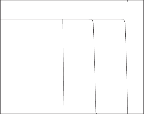
u(x,0) = 10.00≤ x ≤ 20; u(x,0) = 020< x ≤ 40 (initial condition)

u(0) = 1; u(40) = 0 (Dirichlet boundary conditions) (2.13.27)

We will integrate this equation using 101 grid points up to a total time of

4 s. Program 2.10 accomplishes this task with the MacCormack explicit method

(2.13.9)–(2.13.10). For right-moving discontinuities such as (2.13.27), it is rec-

ommended to use only forward differences in the direction of discontinuity

AN APPLICATION TO BIOLOGICAL FLUID DYNAMICS: FLOW IN AN ELASTIC TUBE 133

0 5 10 15 20 25 30 35 40 45

t = 0 t = 2 s t = 4 s

FIGURE 2.13.1 MacCormack explicit scheme for the nonlinear convection equation;

C = 1.0.

propagation (Tennehill et al., 1997, p. 187). Hence, in Program 2.10, differ-

ence switching was not implemented. Results are plotted in Figs. 2.13.1–2.13.3

at various time levels for three different values of C .ForC = 1 (Fig. 2.13.1) the

solution is completely free of dispersion and dissipation errors as it progresses

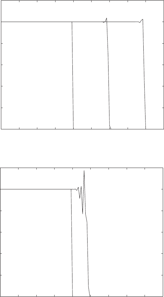
on the characteristics. However, as we observe in Fig. 2.13.2, when the Courant

number is reduced to 0.75, numerical stability is maintained, but the solution

displays signiﬁcant dispersion errors in the vicinity of the discontinuity. Finally,

when C = 1.1 (Fig. 2.13.3), which violates the linear stability limit of C ≤ 1,

the solution deteriorates and, as expected, becomes unstable.

Next, in Program 2.11 the same equation (2.13.27) is solved with the implicit

Beam and Warming method (2.13.19), for C = 1. We note that (2.13.19) written

for all the interior grid points results in a system of linear equations where the

coefﬁcient matrix is triadiagonal. A very efﬁcient compact storage algorithm for

solving such systems is the Thomas algorithm (see Section 4.4) included as a

MATLAB function script in Program 2.11. It is also possible to solve the resulting

linear system using the MATLAB “backslash” multiplication function (which

we provide as an option in Program 2.11). We also note that in this program,

the equations have been modiﬁed by the inclusion of the artiﬁcial dissipation

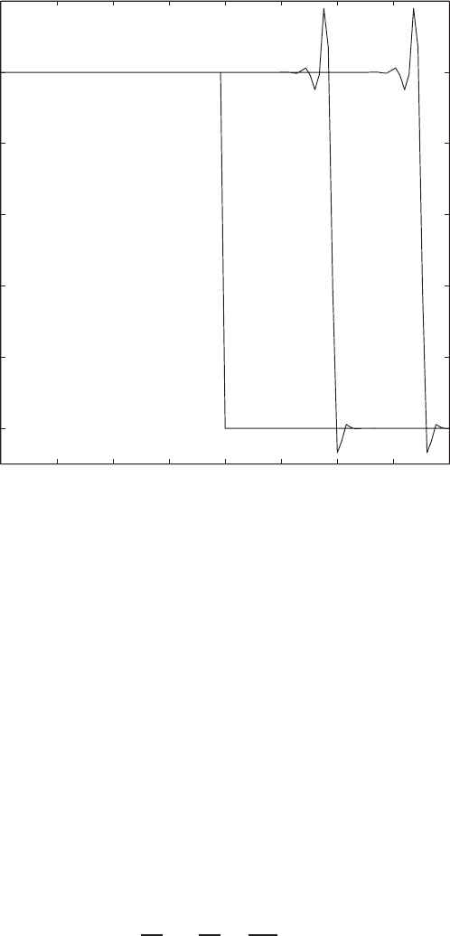
term (2.13.12) to stabilize the solution, with ω = 0.8. Figure 2.13.4 displays the

results for C = 1. Although the solution is stable and does not have signiﬁcant

134 INVISCID FLUID FLOWS

0 5 10 15 20 25 30 35 40 45

t = 0

t = 2 s

t = 4 s

FIGURE 2.13.2 MacCormack explicit scheme for the nonlinear convection equation;

C = 0.75.

0 5 10 15 20 25 30 35 40 45

t = 0

t = 0.836 s

FIGURE 2.13.3 MacCormack explicit scheme for the nonlinear convection equation;

C = 1.1.

AN APPLICATION TO BIOLOGICAL FLUID DYNAMICS: FLOW IN AN ELASTIC TUBE 135

0 5 10 15 20 25 30 35 40

t = 0

t = 2 s

t = 3.6 s

FIGURE 2.13.4 Beam and Warming solution for the nonlinear convection equation; ω = 0.8.

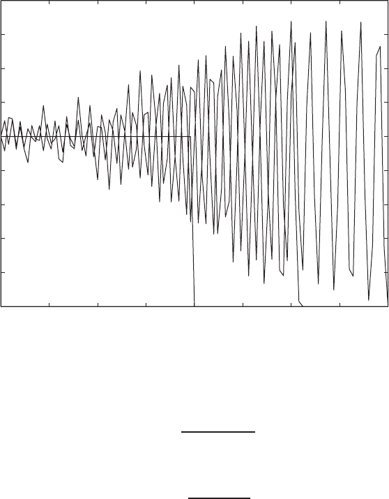
dissipation errors, it is degraded by the existence of signiﬁcant dispersion errors

in the vicinity of the discontinuity. When ω = 0, Fig. 2.13.5. shows that the

solution becomes unstable and numerical errors amplify exponentially. Hence,

for the inviscid, nonlinear convection equation, the implicit Beam and Warming

method may not be the best choice.

Problem 2.12 The one-dimensional Burgers equation (2.13.20) with ν as the

kinematic viscosity serves as a model equation for physical problems in ﬂuid

dynamics ranging from strong shock waves to spectral dynamics of turbulence.

It has also several exact (closed form) solutions for highly viscous, low Reynolds

number ﬂows. For such ﬂows, we can use nondimensional variables by making

the substitutions:

x/L → x, νt/L

→ t, uL/ν → u (2.13.28)

With this scaling, (2.13.20) becomes

∂u

∂t

∂u

∂x

∂

∂x

(2.13.29)

136 INVISCID FLUID FLOWS

0 5 10 15 20 25 30 35 40

FIGURE 2.13.5 Beam and Warming solution for the nonlinear convection equation; ω = 0.

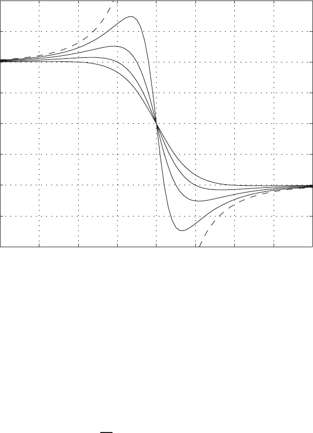
A family of solutions for this equation is obtained by Benton and Platzman

(1972), one of which is given as

u(x, t) =

−2sinhx

cosh x −e

−t

(2.13.30)

As t → 0, (2.13.30) gives

u(x,0) =

−2sinhx

cosh x −1

(2.13.31)

and as t →∞(steady state), one obtains

u(x, t) =−2tanhx (2.13.32)

The exact solution, (2.13.30), is discontinuous at x = 0att = 0 and, owing to

the second-order diffusion term in (2.13.29), the discontinuity is rapidly smoothed

in time. The exact solution (2.13.30) is valid for the initial value problem for

−∞ ≤ x ≤+∞and to use it for testing numerical schemes, we will deﬁne

initial/boundary conditions for ﬁnite x. Consequently, the numerical solution will

be approximate.

Initial conditions can be gotten directly from (2.13.31) and we can deﬁne the

integration domain as −6 ≤ x ≤+6 with boundary conditions of either Dirichlet

AN APPLICATION TO BIOLOGICAL FLUID DYNAMICS: FLOW IN AN ELASTIC TUBE 137

−4 −3 −2 −1 0 1 2 3 4

−4

−3

−2

−1

FIGURE 2.13.6 Exact solution (2.13.30) for the Burgers equation: t = 0 (dash), 0.2, 0.5,

1, 2.

or Neumann type. At these boundary points, Dirichlet boundary conditions are

u(x,0) =∓2.0atx =±6. Neumann boundary conditions are prescribed on the

gradient of u, and will be given below.

Problem 2.13 Integrate (2.13.29) using the fully explicit MacCormack method.

Generate the initial conditions from (2.13.31). Use 100 evenly spaced grid points

within −6 ≤ x ≤+6, and implement Neumann boundary conditions, i.e.,

∂u

∂x

= 0atx =±6. (2.13.33)

It is sufﬁcient to approximate the gradient boundary conditions using ﬁrst-order

one-sided differences. The fully explicit MacCormack scheme must satisfy

max

t/x ≤ 1 (convective stability) and t/x

≤ 1/2 (viscous stability)

restrictions in choosing the allowable time step, t. Choose your time step so

that both conditions will be satisﬁed. Here, u

max

is the maximum velocity at

t = 0. Compare your solution with the exact solution at t = 0.2, 0.5, 1, 2.

138 INVISCID FLUID FLOWS

Problem 2.14 Use the fully implicit Beam and Warming method to obtain a

numerical solution to (2.13.29), with the same boundary-initial conditions as in

Problem 2.13 with 100 grid points. Note that there is no stability restriction

because we are using the fully implicit formula. Perform this calculation with

Dirichlet boundary conditions u(x,0) =∓2.0atx =±6. Compare the numerical

results with the exact solution at t = 0.2, 0.5, 1, 2. What is the effect of adding

artiﬁcial viscosity such as (2.13.12)? What is the effect of C > 1? How does the

solution compare with the MacCormack solution for this problem?

We now return to the elastic tube problem, and write (2.13.1) and (2.13.2) in

conservative vector–matrix form:

∂U

∂t

∂F

∂z

= Q (2.13.34)

where the vectors U, F,andQ are deﬁned as

U =

, F =

⎡

⎣

⎤

⎦

, Q =

⎡

⎢

⎣

−ψ

f −

∂p

∂z

⎤

⎥

⎦

Using the MacCormack explicit method consisting of a forward-difference

predictor step and a backward-difference corrector, (2.13.34) can be advanced in

time in the following manner:

= U

−

t

z

i+1

−F

) + tQ

(2.13.35)

= U

−

t

z

(

−F

i−1

) +tQ

(2.13.36)

The value of the unknowns at the advanced time level then can be calculated

from

n+1

(

) (2.13.37)

In (2.13.35)–(2.13.37), index i represents position in space, and the index n

is for the time level. For this problem, we recommend implementing operator

switching in space, alternating from backward/forward to forward/backward dur-

ing consecutive time steps. As the equation is hyperbolic, numerical stability

requires Courant number (C ) to be less than one, such that the computation must

obey

C =

max

t

z

≤ 1 (2.13.38)

where V

max

is the maximum velocity at a given time step.

It should be noted that although the algorithm is written in the compact

vector–matrix form of (2.13.35)–(2.13.37), in practice, time advancement is done

AN APPLICATION TO BIOLOGICAL FLUID DYNAMICS: FLOW IN AN ELASTIC TUBE 139

separately for each equation in a sequential manner. The application that we con-

sider here consists of a generic elastic tube of reference length L = 25 cm. We

use ﬂuid properties relevant to human blood, such as density, ρ = 1.06 g/cm

;

viscosity, μ = 0.049 poise. The reference pressure is set to p

= 80 mmHg.

The proximal boundary condition for pressure, p

(t), is time varying while

the distal boundary condition is ﬁxed at 15 mmHg. The reference pressure p

represents the approximate maximum pressure in the system. Velocity boundary

conditions are obtained by zeroth-order extrapolation at both ends of the vessel.

We adopt an approximate equation of state, S (p, z):

S (p, z) = 7.07e

−0.25z+(p−p

)/ρc(p, z )c(p

, z )

(2.13.39)

It is apparent that this expression depends on c, the wave speed in the ﬂuid.

Assuming that c is a product of linear functions of both z and p andisinunits

of cm/s, an equation for this quantity can be written as (Anliker et al., 1971)

c(p, z) = (97 + 2.03p)(1 +0.02z) (2.13.40)

The pulsating ﬂow in the elastic tube is assumed to be laminar and unsteady,

so that the friction term, f , can be written using Poiseuille’s formula for circular

pipes:

laminar

=−8π

(2.13.41)

This equation will approximate viscous effects in the vessel and is assumed valid

for both steady and unsteady ﬂow.

Initial conditions are less important because after a few initial cycles driven

by the proximal boundary conditions, the solution reaches quasi-steady state

independent of the initial conditions. If the initial conditions are not too different

than the ﬁnal solution, the computation time to reach quasi steady state will

decrease. For this computation, we implemented the following initial conditions:

V = V





(2.13.42)

p = p





(2.13.43)

Here, V

= 0.1cm/s,V

= 3.0cm/s,p

= 15 mmHg, and p

is obtained from

the proximal boundary condition for pressure.

The axial z direction is discretized with 100 points, corresponding to a grid

spacing of z = 0.25. We impose a forcing pressure pulse of about 86 beats per

minute through the proximal boundary condition. The signal is interpolated by

a cubic spline to provide the value of the left boundary condition for pressure

140 INVISCID FLUID FLOWS

0 0.1 0.2 0.3 0.4 0.5 0.6 0.7

time [s]

Pressure [mmHg]

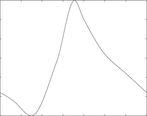
FIGURE 2.13.7 Proximal pressure boundary condition.

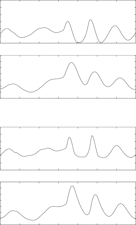
at each time step. Figure 2.13.7 shows a typical input signal for the proximal

pressure boundary condition and Fig. 2.13.8 displays the calculated pressure and

velocity at several locations along the axial direction, z. Closer to the left bound-

ary (Fig. 2.13.8a), the velocity plot indicates reverse ﬂow in the vessel, which

disappears downstream. Localized regions of backﬂow have been observed in

other studies as well. As we advance downstream (Fig. 2.13.8 b, c), both the local

maximum and minimum velocity magnitudes increase and the velocity is com-

pletely synchronous with the pressure. Both quantities remain periodic, although

they produce higher harmonics of the forcing pressure. All these qualitative obser-

vations are compatible with other models for various arterial simulations, but we

stress the fact that the example we are presenting here is for a generic elastic

tube; it has to be adapted to real life arterial blood ﬂow by matching all the

constants in the mathematical model to actual measured values, and many other

factors have to be considered to improve the model for applicability to realistic

simulations concerning arterial blood ﬂow. For example, what is the effect of

viscosity? Is the Poiseuille friction factor adequate? Should turbulence be con-

sidered? Is the wall elasticity modeled with sufﬁcient accuracy? Are the proximal

and distal boundary conditions sufﬁciently accurate to model the physical prob-

lem? Regardless, the model outlined in this section should serve as a starting

point for simulating arterial blood ﬂow (Akman, Biringen, and Waggy, 2011).

AN APPLICATION TO BIOLOGICAL FLUID DYNAMICS: FLOW IN AN ELASTIC TUBE 141

1.4 1.5 1.6 1.7 1.8 1.9 2 2.1

−20

100

Velocity [cm/s]

1.4 1.5 1.6 1.7 1.8 1.9 2 2.1

100

110

time [s]

z = 15 cm

(a)

(b)

z = 20 cm

Pressure [mmHg]

1.4 1.5 1.6 1.7 1.8 1.9 2 2.1

−20

100

Velocity [cm/s]

1.4 1.5 1.6 1.7 1.8 1.9 2 2.1

100

110

time [s]

Pressure [mmHg]

FIGURE 2.13.8 Pressure and velocity signals over one period of the proximal pressure

cycle. (a) z = 15 cm; (b) z = 20 cm; (c) z = 22 cm.