Bichop R.H. (Ed.) Mechatronic Systems, Sensors, and Actuators: Fundamentals and Modeling

Подождите немного. Документ загружается.

14-2 Mechatronic Systems, Sensors, and Actuators

fundamental approaches which will eventually lead to successful MEMS simulations becoming routine.

We also survey available tools which a MEMS developer can use to achieve good simulation results. Many

of these tools build MEMS development systems on platforms already in existence for other technologies,

thus leveraging the extensive resources which have gone into previous development and avoiding “rein-

venting the wheel.”

For our discussion of modeling and simulation, the salient characteristics of MEMS are:

1. Inclusion and interaction of multiple domains and technologies

2. Both two- and three-dimensional behaviors

3. Mixed digital (discrete) and analog (continuous) input, output, and signals

4. Micro- (or nano-) scale feature sizes

Techniques for the manufacture of reliable (two-dimensional) systems with micro- or nano-scale feature

sizes (Characteristic 4) are very mature in the field of microelectronics, and it is logical to attempt to extend

these techniques to MEMS, while incorporating necessary changes to deal with Characteristics 1–3. Here

we survey some of the major principles which have made microelectronics such a rapidly evolving field,

and we look at microelectronics tools which can be used or adapted to allow us to apply these principles

to MEMS. We also discuss why applying such strategies to MEMS may not always be possible.

14.2 The Digital Circuit Development Process: Modeling

and Simulating Systems with Micro- (or Nano-) Scale

Feature Sizes

A typical VLSI digital circuit or system process flow is shown in Figure 14.1, where the dotted lines show

the most optimistic point to which the developer must return if errors are discovered. Option A, for a

“mature” technology, is supported by efficient and accurate simulators, so that even the first actual

implementation (“first silicon”) may have acceptable performance. As a process matures, the goal is to

have better and better simulations, with a correspondingly smaller chance of discovering major perfor-

mance flaws after implementation. However, development of models and simulators to support this goal

is in itself a major task. Option B (immature technology), at its extreme, would represent an experimental

technology for which not enough data are available to support even moderately robust simulations. In

modern software and hardware development systems, the emphasis is on tools which provide increasingly

good support for the initial stages of this process. This increases the probability that conceptual or design

errors will be identified and modifications made as early in the process as possible and thus decreases

both development time and overall development cost.

At the microlevel, the development cycle represented by Option A is routinely achieved today for many

digital circuits. In fact, the entire process can in some cases be highly automated, so that we have “silicon

compilers” or “computers designing computers.” Thus, not only design analysis, but even design synthesis

is possible. This would be the case for well-established silicon-based CMOS technologies, for example.

There are many characteristics of digital systems which make this possible. These include:

•

Existence of a small set of basic digital circuit elements. All Boolean functions can be realized by

combinations of the logic functions AND, OR, NOT. In fact, all Boolean functions can be realized

by combinations of just one gate, a NAND (NOT-AND) gate. So if a “model library” of basic

gates (and a few other useful parts, such as I/O pins, multiplexors, and flip-flops) is developed,

systems can be implemented just by combining suitable library elements.

•

A small set of standardized and well-understood technologies, with well-characterized fabrication

processes that are widely available. For example, in the United States,

the MOSIS service [3]

provides access to a range of such technologies. Similar services elsewhere include CMP in France

[4], Europractice in Europe [5], VDEC in Japan [6], and CMC in Canada [7].

•

A well-developed educational infrastructure and prototyping facilities. These are provided by all of

the services listed above. These types of organization and educational support had their origins in

9258_C014.fm Page 2 Tuesday, October 2, 2007 1:06 AM

Modeling and Simulation for MEMS 14-3

the work of Mead and Conway [8] and continue to produce increasingly sophisticated VLSI engi-

neers. An important aspect of this infrastructure is that it also provides, at relatively low cost, access

to example devices and systems, made with stable fabrication processes, whose behavior can be tested

and compared to simulation results, thereby enabling improvements in simulation techniques.

•

“Levels and views” (abstraction and encapsulation or “information hiding”) (see [9]). This concept

is illustrated in Figure 14.2a. For the VLSI domain, we can identify at least five useful levels of

abstraction, from the lowest (layout geometry) to the highest (system specification). We can also

“view” a system behaviorally, structurally, or physically. In the behavioral domain we describe the

functionality of the circuit without specifying how this functionality will be achieved. This allows us

to think clearly about what the system needs to do, what inputs are needed, and what outputs will

be provided. Thus we can view the component as a “black box” that has specified responses to given

inputs. The current through a MOS field effect transistor (MOSFET), given as a function of the

gate voltage, is a (low-level) behavioral description, for example. In the physical domain we specify

the actual physical parts of the circuit. At the lowest levels in this domain, we must choose what

material each piece of the circuit will be made from (for example, which pieces of wire will lie in

each of the metal layers usually provided in a CMOS circuit) and exactly where each piece will be

placed in the actual physical layout. The physical description will be translated directly into mask

layouts for the circuit. The structural domain is intermediate between physical and behavioral. It

provides an interface between the functionality specified in the behavioral domain, which ignores

geometry, and the geometry specified in the physical domain, which ignores functionality. In this

intermediate domain, we can carry out logic optimization and state minimization, for example.

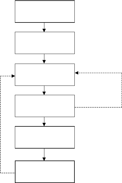
FIGURE 14.1 Product design process. A: mature technology, B: immature technology.

Testing

Product

Requirements

Product

Specifications

Design

Simulation

Implementation

9258_C014.fm Page 3 Tuesday, October 2, 2007 1:06 AM

14-4 Mechatronic Systems, Sensors, and Actuators

A schematic diagram is an example of a structural description. Of course, not all circuit charac-

teristics can be completely encapsulated in a single one of these views. For example, if we change

the physical size of a wire, we will probably affect the timing, which is a behavioral property. The

principle of encapsulation leads naturally to the development of extensive IP (intellectual prop-

erty), that is, libraries of increasingly sophisticated components that can be used as “black boxes”

by the system developer.

•

Well-developed models for basic elements that clearly delineate effects due to changes in design,

fabrication process, or environment. For example, in [10], the factors in the basic first-order equa-

tions for I

, the drain-to-source current in an NMOS transistor, can clearly be divided into those

under the control of the designer (W/L, the width-to-length ratio for the transistor channel), those

dependent on the fabrication process (

, the permittivity of the gate insulator, and t

, the thickness

of the gate insulator), those dependent on environmental factors (V

and V

, the drain-to-source

and gate-to-source voltages, respectively), and those that are a function of both the fabrication

process and the environment (

, the effective surface mobility of the carriers in the channel, and V

the threshold voltage). More detailed information on modeling MOSFETs can be found in [11].

Identification of fundamental parameters in one stage of the development process can be of great

value in other stages. For example, the minimum feature size

for a given technology can be used

to develop a set of “design rules” that express mandatory overlaps and spacings for the different

physical materials. A design tool can then be developed to “enforce” these rules, and the conse-

quences can be used to simplify, to some extent, the modeling and simulation stages. The parameter

can also be used to express effects due to scaling when scaling is valid.

FIGURE 14.2 A taxonomy for component development (“levels and views”): (a) standard VLSI classifications,

(b) a partial classification for MEMS components.

Levels Views

Behavioral Structural Physical

Performance

specifications

CPUs, memory,

switches, controllers,

buses

Physical

partitions

Algorithms

Modules,

data structures

Clusters

ALUs, MUXs,

registers

Floorplans

Boolean equations,

FSMs

Gates,

flip-flops

Cells,

modules

Transfer functions,

timing

Transistors, wires,

contacts, vias

Layout

geometry

(a)

(b)

Levels Views

Behavioral Structural Physical

Performance

specifications

Sensors,

actuators,

systems

Physical

partitions

Multiple energy

domain

components

Clusters

Domain-domain

components

Floorplans

Single energy

domain

components

Cells,

modules

Layout

geometry

Transfer functions,

timing

Beams,

membranes, holes,

grooves, joints

9258_C014.fm Page 4 Tuesday, October 2, 2007 1:06 AM

Modeling and Simulation for MEMS 14-5

•

Mature tools for design and simulation, which have evolved over many generations and for which

moderately priced versions are available from multiple sources. For example, many of today’s tools

incorporate versions of the design tool MAGIC [12] and the simulator SPICE (Simulation Program

with Integrated Circuit Emphasis) [13], both of which were originally developed at the University

of California, Berkeley. Versions of the SPICE simulator typically support several device models

(currently, for example, six or more different MOS models and five different transmission line

models), so that a developer can choose the level of device detail appropriate to the task at hand.

Free or low-cost versions of both MAGIC and SPICE, as well as extended versions of both tools, are

widely available. Many different techniques, such as model binning (optimizing models for specific

ranges of model parameters) and inclusion of proprietary process information, are employed to

produce better models and simulation results, especially in the HSPICE version of SPICE and in

other high-end versions of these tools [11].

•

Integrated development systems that are widely available and that provide support for a variety

of levels and views, extensive component libraries, user-friendly interfaces and online help, as well

as automatic translation between domains, along with error and constraint checking. In an inte-

grated VLSI development system, sophisticated models, simulators, and translators keep track of

circuit information for multiple levels and views, while allowing the developer to focus on one

level or view at a time. Many development systems available today also support, at the higher

levels of abstraction, structured “programming” languages such as VHDL (Very Large Scale Inte-

grated Circuit Hardware Description Language) [14,15] or Verilog [16].

A digital circuit developer has many options, depending on performance constraints, number of units to

be produced, desired cost, available development time, etc. At one extreme the designer may choose to

develop a “custom” circuit, creating layout geometries, sizing individual transistors, modeling RC effects

in individual wires, and validating design choices through extensive low-level SPICE-based simulations.

At the other extreme, the developer can choose to produce a PLD (programmable logic device), with a

predetermined basic layout geometry consisting of cells incorporating programmable logic and storage

(Figure

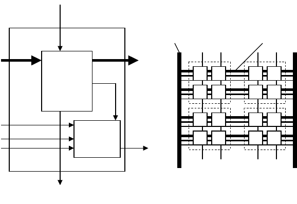
14.3) that can be connected as needed to produce the desired device functionality. A high end PLD

may contain as many as 100,000 (100 K) cells similar to the one in Figure 14.3 and an additional 100 K

bytes of RAM (random access memory) storage. In an integrated development system, such as those

FIGURE 14.3 A generic programmable logic device architecture.

Carry-in

Mem

out

Carry-out

Generic pld cell

bus

Out

bus

Clock

Reset

Mem in

Global

bus

Local

bus

Block of pld cells

Logic

(look-up

table)

Memory

(1-bit)

(a) (b)

9258_C014.fm Page 5 Tuesday, October 2, 2007 1:06 AM

14-6 Mechatronic Systems, Sensors, and Actuators

provided by References 17 and 18, the developer enters the design in either schematic form or a high level

language, and then the design is automatically “compiled” and mapped to the PLD geometry, and func-

tional and timing simulations can be run. If the simulation results are acceptable, an actual PLD can then

be programmed directly, as a further step in the development process, and even tested, to some extent,

with the same set of test data as was used for the simulation step. This “rapid prototyping” [19] for the

production of a “chip” is not very different from the production of a working software program (and the

PLD can be reprogrammed if different functionality is later desired). Such a system, of course, places many

constraints on achievable designs. In addition, the automated steps, which rely on heuristics rather than

exact techniques to find acceptable solutions to the many computationally complex problems that need

to be solved during the development process, sacrifice performance for ease of development, so that a

device designed in such a system will never achieve the ultimate performance possible for the given

technology. However, the trade-offs include ease of use, much shorter development times, and the man-

agement of much larger numbers of individual circuit elements than would be possible if each individual

element were tuned to its optimum performance. In addition, if a high-level language is used for input,

an acceptable design can often be translated, with few changes, to a more powerful design system that will

allow implementation in more flexible technologies and additional fine tuning of circuit performance. In

Figure 14.4 we see some of the levels of abstraction which are present in such a development

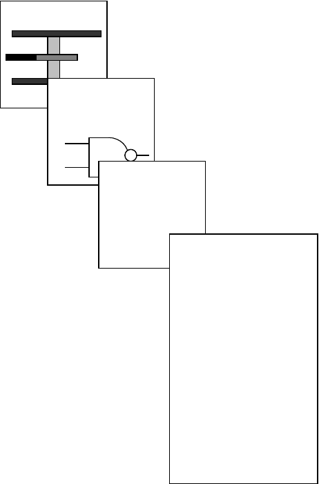
FIGURE 14.4 Levels of abstraction—half adder.

Transistor

(physical view)

Library

component

(phys. / behav./

struct.)

Netlist

(structural)

n1: a b o1

n3: o1 o2 o3

VHDL

entity HALFADDER is

port (A,B: in bit;

S,COUT: out bit);

end ADDER;

architecture A of HALFADDER is

component XOR

port (X1,X2: in bit; O: out bit);

end component;

component AND

port (X1,X2: in bit; O: out bit);

end component;

begin

G1: XOR

port map (A,B,S);

G2: AND

port map (A,B,COUT);

end A;

n2: a c o2

9258_C014.fm Page 6 Tuesday, October 2, 2007 1:06 AM

Modeling and Simulation for MEMS 14-7

process, with the lowest level being detailed transistor models and the highest a VHDL description of a

half adder.

14.3 Analog and Mixed-Signal Circuit Development: Modeling

and Simulating Systems with Micro- (or Nano-) Scale

Feature Sizes and Mixed Digital (Discrete) and Analog

(Continuous) Input, Output, and Signals

At the lowest level, digital circuits are in fact analog devices. A CMOS inverter, for example, does not

“switch” instantaneously from a voltage level representing binary 0 to a voltage level representing binary

1. However, by careful design of the inverter’s physical structures, it is possible to make the switching

time from the range of voltage outputs which are considered to be “0” to the range considered to be “1”

(or vice versa) acceptably short. In MOSFETs, for example, the two discrete signals of interest can be

identified with the transistor, modeled as a switch, being “open” or “closed,” and the “switching” from one

state to another can be ignored except at the very lowest levels of abstraction. In much design and simulation

work, the analog aspects of the digital circuit’s behavior can thus be ignored. Only at the lower levels of

abstraction will the analog properties of VLSI devices or the quantum effects occurring, e.g., in a MOSFET

need to be explicitly taken into account, ideally by powerful automated development tools supported by

detailed models. At higher levels this behavior can be encapsulated and expressed in terms of minimum

and maximum switching times with respect to a given capacitive load and given voltage levels. Even in

digital systems, however, as submicron feature sizes become more common, more attention must be paid

to analog effects. For example, at small feature sizes, wire delay due to RC effects and crosstalk in nearby

wires become more significant factors in obtaining good simulation results [20]. It is instructive to examine

how simulation support for digital systems can be extended to account for these factors.

Typically, analog circuit devices are much more likely to be “hand-crafted” than digital devices. SPICE

and SPICE-like simulations are commonly used to measure performance at the level of transistors, resistors,

capacitors, and inductors. For example, due to the growing importance of wireless and mobile computing,

a great deal of work in analog design is currently addressing the question of how to produce circuits

(digital, analog, and mixed-signal) that are “low-power,” and simulations for devices to be used in these

circuits are typically carried out at the SPICE level. Unless a new physical technology is to be employed,

the simulations will mostly rely on the commonly available models for transistors, transmission lines, etc.,

thus encapsulating the lowest level behaviors.

Let us examine the factors given above for the success of digital system simulation and development to

see how the analog domain compares. We assume a development cycle similar to that shown in Figure 14.1.

•

Is there a small set of basic circuit elements? In the analog domain it is possible to identify sets of

components, such as current mirrors, op-amps, etc. However, there is no “universal” gate or small

set of gates from which all other devices can be made, as is true in the digital domain. Another

complicating factor is that elementary analog circuit elements are usually defined in terms of

physical performance. There is no clean notion of 0/1 behavior. Because analog signals are con-

tinuous, it is often much more difficult to untangle complex circuit behaviors and to carry out

meaningful simulations where clean parameter separations give clear results. Once a preliminary

analog device or circuit design has been developed, the process of using simulations to decide on

exact parameter values is known as “exploring the design space.” This process necessarily exhibits

high computational complexity. Often heuristic methods such as simulated annealing, neural nets,

or a genetic algorithm can be used to perform the necessary search efficiently [21].

•

Is there a small set of well-understood technologies? In this area, the analog and mixed signal

domain is similar to the digital domain. Much analog development activity focuses on a few

standard and well-parameterized technologies. In general, analog devices are much more sensi-

tive to variations in process parameters, and this must be accounted for in analog simulation.

9258_C014.fm Page 7 Tuesday, October 2, 2007 1:06 AM

14-8 Mechatronic Systems, Sensors, and Actuators

Statistical techniques to model process variation have been included, for example, in the APLAC

tool [22], which supports object-oriented design and simulation for analog circuits. Modeling

and simulation methods, which incorporate probabilistic models, will become increasingly impor-

tant as nanoscale devices become more common and as new technologies depending on quantum

effects and biology-based computing are developed. Several current efforts, for example, are

aimed at developing a “BIOSPICE” simulator, which would incorporate more stochastic system

behavior [23].

•

Is there a well-developed educational infrastructure and prototyping facilities? All the organiza-

tions, which support education and prototyping in the digital domain [3–7], provide similar

support for analog and mixed-signal design.

•

Are encapsulation and abstraction widely employed? In the past few years, a great deal of progress

has been made in incorporating these concepts into analog and mixed-signal design systems. The

wide availability of very powerful computers, which can perform the necessary design and simu-

lation tasks in reasonable amounts of time, has helped to make this progress possible. In [24], for

example, top-down, constraint-driven methods are described, and in [25] a rapid prototyping

method for synthesizing analog and mixed signal systems, based on the tool suite VASE (VHDL-

AMS Synthesis Environment), is demonstrated. These methods rely on classifications similar to

those given for digital systems in Figure 14.2a.

•

Are there well-developed models, mature tools, and integrated development systems which are widely

available? In the analog domain, there is still much more to be done in these areas than in the digital

domain, but prototypes do exist. In particular, the VHDL and Verilog languages have been extended

to allow for analog and mixed-signal components. The VHDL extension, e.g., VHDL-AMS [14], will

allow the inclusion of any algebraic or ordinary differential equation in a simulation. However, there

does not exist a completely functional VHDL-AMS simulator, although a public domain version,

incorporating many useful features, is available at [26] and many commercial versions are under

development (e.g., [27]). Thus, at present, expanded versions of MAGIC and SPICE are still the most

widely-used design and simulation tools. While there have been some attempts to develop design

systems with configurable devices similar to the digital devices shown in Figure 14.3, these have not

so far been very successful. Currently, more attention is being focused on component-based devel-

opment with design reuse for SOC (systems on a chip) through initiatives such as [28].

14.4 Basic Techniques and Available Tools for MEMS

Modeling and Simulation

Before trying to answer the above questions for MEMS, we need to look specifically at the tools and

techniques the MEMS designer has available for the modeling and simulation tasks. As pointed out in

[29,30], the bottom line is, in any simulator, all models are not created equal. The developer must be

very clear about what parameters are of greatest interest and then must choose the models and simulation

techniques (including implementation in a tool or tools) that are most likely to give the most accurate

values for those parameters in the least amount of simulation time. For example, the model used to

determine static behavior may be different from the model needed for an adequate determination of

dynamic behavior. Thus, it is useful to have a range of models and techniques available.

14.4.1 Basic Modeling and Simulation Techniques

We need to make the following choices:

•

What kind of behavior are we interested in? IC simulators, for example, typically support DC

operating analysis, DC sweep analysis (stepping current or voltage source values) and transient

sweep analysis (stepping time values), along with several other types of transient analysis [30].

9258_C014.fm Page 8 Tuesday, October 2, 2007 1:06 AM

Modeling and Simulation for MEMS 14-9

•

Will the computation be symbolic or numeric?

•

Will use of an exact equation, nodal analysis, or finite element analysis be most appropriate?

Currently, these are the techniques which are favored by most MEMS developers.

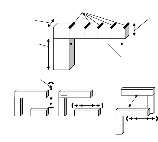
To show what these choices entail, let us look at a simple example that combines electrical and mechanical

parts. The cantilever beam in Figure 14.5a, fabricated in metal, polysilicon, or a combination, may be

combined with an electrically isolated plate to form a parallel plate capacitor. If a mechanical force or a varying

voltage is applied to the beam (Figure 14.5b1), an accelerometer or a switch can be obtained [31]. If instead

the plate can be moved back and forth, a more efficient accelerometer design results (Figure 14.5b2); this is

the basic design of Analog Devices’ accelerometer, probably the first truly successful commercial MEMS

device [32,33]. If several beams are combined into two “combs,” a comb-drive sensor or actuator results,

as in Figure 14.5b3 [34]. Let us consider just the simplest case, as shown in Figure 14.5b1.

If we assume the force on the beam is concentrated at its end point, then we can use the method of [35]

to calculate the “pull-in” voltage, that is, the voltage at which the plates are brought together, or to a stopper which

keeps the two plates from touching. We model the beam as a dampened spring-mass system and look for

the force

, which, when translated into voltage, will give the correct

value for the beam to be “pulled in.”

F = mx′′ + Bx′ + kx

Here mass

WTL

, where

is the density of the beam material,

/12 is the moment of inertia,

= 3

is the Young’s modulus of the beam material, and

(

)

1/4

. This second-order linear

differential equation can be solved numerically to obtain the pull-down voltage. In this case, since a closed

form expression can be obtained for

, symbolic computation would also be an option. In Reference 36 it

is shown that for this simple problem several commonly used methods and tools will give the same result,

as is to be expected.

To obtain a more accurate model of the beam we can use the method of nodal analysis, that treats the

beam as a graph consisting of a set of edges or “devices,” linked together at “nodes.” Nodal analysis

assumes that at equilibrium the sum of all values around each closed loop (the “across” quantities) will

FIGURE 14.5 Cantilever beam and beam–capacitor options: (a) cantilever beam dimensions, (b) basic beam–

capacitor designs.

“nodes”

Width W Thickness T

Height H

Length L

Displacement x

(b1) Vertical (b2) Horizontal (b3) Side by side

(a)

(b)

9258_C014.fm Page 9 Tuesday, October 2, 2007 1:06 AM

14-10 Mechatronic Systems, Sensors, and Actuators

be zero, as will the sum of all values entering or leaving a given node (the “through” quantities). Thus,

for example, the sum of all forces and moments on each node must be zero, as must the sum of all

currents flowing into or out of a given node. This type of modeling is sometimes referred to as “lumped

parameter,” since quantities such as resistance and capacitance, which are in fact distributed along a

graph edge, are modeled as discrete components. In the electrical domain Kirchhoff ’s laws are examples of

these rules. This method, which is routinely applied to electrical circuits in elementary network analysis

courses (see, e.g., [37]), can easily be applied to other energy domains by using correct domain equivalents

(see, e.g., [38]). A comprehensive discussion of the theory of nodal analysis can be found in [39]. In Figure

14.5a, the cantilever beam has been divided into four “devices,” subbeams between node i and i + 1, i =

1, 2, 3, 4, where the positions of nodes i and i + 1 are described by (x

, y

) and (x

i+1

, y

i+1

) the

coordinates and slope at P

and P

i+1

. The beam is assumed to have uniform width W and thickness T, and

each subbeam is treated as a two-dimensional structure free to move in three-space. In [40] a modified

version of nodal analysis is used to develop numerical routines to simulate several MEMS behaviors,

including static and transient behavior of a beam-capacitor actuator. This modified method also adds

position coordinates z

and z

i+1

and replaces the slope

at each node with a vector of slopes,

, and

, giving each node six degrees of freedom.

Since nodal analysis is based on linear elements represented as the edges in the underlying graph, it cannot

be used to model many complex structures and phenomena such as fluid flow or piezoelectricity. Even for

the cantilever beam, if the beam is composed of layers of two different materials (e.g., polysilicon and metal),

it cannot be adequately modeled using nodal analysis. The technique of finite element analysis (FEA) must

be used instead. For example, in some follow-up work to that reported in [36], nodal analysis and symbolic

computation gave essentially the same results, but the FEA results were significantly different. Finite element

analysis for the beam begins with the identification of subelements, as in Figure 14.5a, but each element is

treated as a true three-dimensional object. Elements need not all have the same shape, for example, tetra-

hedral and cubic “brick” elements could be mixed together, as appropriate. In FEA, one cubic element now

has eight nodes, rather than two (Figure 14.6), so computational complexity is increased. Thus, developing

efficient computer software to carry out FEA for a given structure can be a difficult task in itself. But this

general method can take into account many features that cannot be adequately addressed using nodal

analysis, including, for example, unaligned beam sections, and surface texture (Figure 14.7). FEA, which

can incorporate static, transient, and dynamic behavior, and which can treat heat and fluid flow, as well as

electrical, mechanical, and other forces, is explained in detail in [41]. The basic procedure is as follows:

•

Discretize the structure or region of interest into finite elements. These need not be homogeneous,

either in size or in shape. Each element, however, should be chosen so that no sharp changes in

geometry or behavior occur at an interior point.

•

For each element, determine the element characteristics using a “local” coordinate system. This

will represent the equilibrium state (or an approximation if that state cannot be computed exactly)

for the element.

•

Transform the local coordinates to a global coordinate system and “assemble” the element equa-

tions into one (matrix) equation.

•

Impose any constraints implied by restricted degrees of freedom (e.g., a fixed node in a mechanical

problem).

•

Solve (usually numerically) for the nodal unknowns.

•

From the global solution, calculate the element resultants.

14.4.2 A Catalog of Resources for MEMS Modeling and Simulation

To make our discussion of the state-of-the-art of MEMS simulation less confusing, we first list some of

the tools and products available. This list is by no means comprehensive, but it will provide us with a

range of approaches for comparison. It should be noted that this list is accurate as of July 2001, but the

MEMS development community is itself developing, with both commercial companies and university

9258_C014.fm Page 10 Tuesday, October 2, 2007 1:06 AM

Modeling and Simulation for MEMS 14-11

FIGURE 14.6 Nodal analysis and finite element analysis.

FIGURE 14.7 Ideal and actual cantilever beams (side view).

Nodes

Nodal analysis/modified nodal analysis

(“linear” elements)

Nodes

Finite element analysis

(three-dimensional elements)

(a)

(b)

Ideal beam

Rough surface

Unaligned sections

Actual beam

(b)

(a)

9258_C014.fm Page 11 Tuesday, October 2, 2007 1:06 AM