Becker W. Advanced Time-Correlated Single Photon Counting Techniques

Подождите немного. Документ загружается.

204 5 Application of Modern TCSPC Techniques

ing the focal quality can be expected to yield a factor of 3 to 5 in fluorescence

intensity.

x Collection of the fluorescence photons through the microscope objective and

diverting the fluorescence signal by a dichroic mirror. With a high NA objec-

tive, this increases the NA of the detection light path. Compared to the test

setup (an 8 mm photocathode in a distance of 20 mm) an increase in detection

efficiency by a factor of 5 to 10 can be expected.

x Matching of the laser wavelength and the absorption maximum of the fluoro-

phores.

All in all, an improvement in the detected count rate by a factor of 10

appears feasi-

ble. If this is correct, two-photon diode-laser-excited fluorescence can be detected

from a large number of marker dyes in biologically relevant concentrations.

5.14.2 Remote Sensing

With a suitable optical system TCSPC is able to record fluorescence decay func-

tions or diffusely reflected laser signals over remarkable distances. The setup

shown in Fig. 5.136 records the fluorescence of chlorophyll in plants over a dis-

tance of several hundred meters.

Laser module

to target

from target

LX90 telescope

Detector 1

Detector 2

Filter

Dichroic

TCSPC module

Router

stop

start

Routing

PC with

650nm, 50 MHz, 0.5 mW, 100 ps

Aperture 20cm

Fig. 5.136 Fluorescence measurement over large distance

A diode laser sends a beam of 100 ps pulses to the target. The repetition rate of

the laser pulses is 50 MHz, the average power 0.5 mW. A 20-cm (8-inch) tele-

scope (Meade LX90 EMC) is used to collect the photons from the target. The

fluorescence and the reflected light are separated by a dichroic mirror and a

700

r15 nm bandpass filter and detected simultaneously by two individual detec-

tors. Consequently, detector 1 detects the diffusely reflected laser, detector 2 the

fluorescence of the leaves.

In spite of the low laser power, the chlorophyll fluorescence can be detected

over a distance of several hundred meters, with count rates of the order of 1,000

photons per second. At a count rate this low the background signal is an important

5.14 Miscellaneous TCSPC Applications 205

issue; reasonable results can be obtained only at night and at a site that does not

suffer from too much light pollution. A typical result is shown in Fig. 5.137.

Fig. 5.137 Scattering (1) and fluorescence (2) of leaves recorded over a distance of 300 m

The telescope and the laser were pointed into a forest approximately 300 m

away. Curve 1 is the laser scattered at the target, curve 2 is the detected fluores-

cence.

It is almost impossible to hit only one leaf over so great a distance. Therefore

the signals from several leaves at different distances are detected. Moreover, the

signal intensity fluctuates considerably on a scale of seconds due to the motion of

the leaves in the wind. However, because the reflectance and the fluorescence

signals are detected simultaneously, the reflectance can be used as an approxima-

tion of the instrument response function. This approach is not absolutely correct

because the reflected photons can also come from nonfluorescent target compo-

nents, but it delivers decay times with reasonable accuracy. The result of a double-

exponential fit is shown in Fig. 5.138.

Fig. 5.138 Double-exponential lifetime fit to the data of Fig. 5.137 in a time window indi-

cated by the cursor lines. Fluorescence, scattering, and convolution of scattering curve with

calculated decay function. Lower part: Residuals of the fit

206 5 Application of Modern TCSPC Techniques

The fit was calculated for the time window indicated by the vertical lines; it de-

livers lifetime components of 49 ps and 476 ps. The fast lifetime components may

contain some scattered laser light. Nevertheless, even the slow component is re-

markably short. The short lifetime can, however, be explained by the fact that the

excitation density was very small. The leaves were therefore perfectly dark-

adapted. Consequently, the reaction pathway remained fully open during the

measurement, and no decrease of photochemical quenching was induced [345].

5.14.3 Laser Ranging

The high time resolution of TCSPC in conjunction with fast detectors can be used

to build up high-resolution ranging or three-dimensional imaging systems. The

system described in [340, 341, 533] uses a 20 ps diode laser, an actively quenched

avalanche photodiode [116] and an SPC

300 TCSPC module. The photons re-

flected from the target and a reference pulse are recorded within the same TAC

range. A slow-scanning procedure is employed, i.e. the photons for one pixel of

the image are collected and the time-of-flight distribution is read out from the

TCSPC module before the scanner proceeds to the next pixel.

The system achieves a distance repeatability of 10 µm and < 30 µm for a 1 m

and 25 m stand-off, respectively. The distance accuracy corresponds to a timing

accuracy of 33 fs and 100 fs. This surprisingly high resolution is obtained by a

fitting algorithm [516] which gives a better accuracy than the usual centroid esti-

mate. The high accuracy is also explained by the fact that the average timing jitter

of a large number of detected photons decreases with the square root of the photon

number. An accuracy this good can only be achieved with a detector of low transit

time spread, efficient cancellation of system drifts, and a TCSPC time channel

width short enough to sample the IRF correctly.

TCSPC modules with sequencing or imaging capability can be used to read out

the data without stopping the measurement, or to acquire the complete image at a

fast scanning rate.

5.14.4 Positron Lifetime Experiments

Positron lifetime measurements can be used to investigate the type and the density

of lattice defects in crystals [293]. In solid materials positrons have a typical life-

time of 300 to 500 ps until they are annihilated by an electron. When positrons

diffuse through a crystal they may be trapped in crystal imperfections. The elec-

tron density in these locations is different from the density in a defect-free crystal.

Therefore, the positron lifetime depends on the type and the density of the crystal

defects. When a positron annihilates with an electron two

J quanta of 511 keV are

emitted. The

J quanta can easily be detected by a scintillator and a PMT.

5.14 Miscellaneous TCSPC Applications 207

The positrons for the lifetime measurement are conveniently obtained from the

decay of

Na. In

Na a 1.27 MeV J quantum is emitted simultaneously with

the positron. This 1.27 MeV quantum is used as the timing reference for the posi-

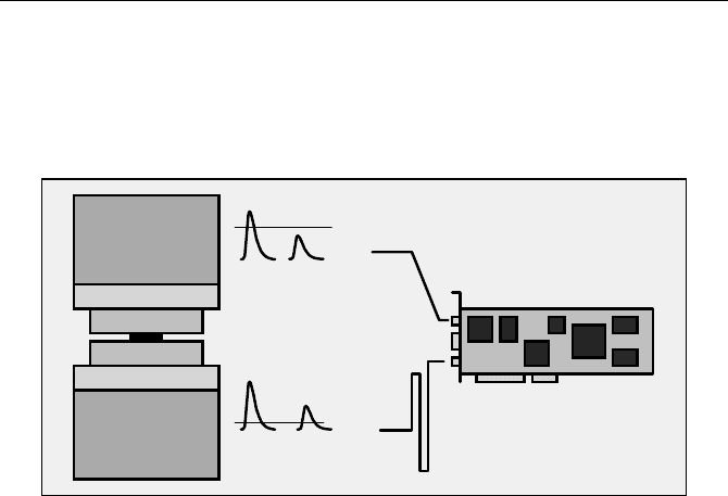
tron lifetime measurement. The general experimental setup is shown in the

Fig. 5.139.

22 Na Source

Sample 1

Sample 2

Scintillator 1

PMT 1

PMT 2

Scintillator 2

Positron

511 keV

22Na

1.27 MeV

Positron

511 keV

22Na

1.27 MeV

start

stop

Delay

TCSPC module

start

stop

threshold

XP 2020

Fig. 5.139 Positron lifetime experiment

The

Na source is placed between two identical samples. Two XP 2020 pho-

tomultipliers equipped with scintillators are attached directly to the two samples.

The pulses from the photomultipliers are used as start and stop pulses for the

TCSPC module. The pulses from PMT 2 are delayed by a few nanoseconds so

that a stop pulse arrives after the corresponding start pulse. Each

J quantum

generates a large number of photons in the scintillator. Therefore, the PMT

pulses are multiphoton signals, and the time resolution can be better than the

transit time spread of the PMTs. Moreover, the amplitudes of the photomultiplier

pulses are proportional to the energy of the particle that caused the scintillation.

Therefore the amplitudes can be used to distinguish between the 511 keV events

of the positron decay and the 1.27 MeV events from the

Na. The discriminator

thresholds for start and stop are adjusted in a way that the stop channel sees all,

the start channel only the larger

Na events. The rate of the

Na events is of the

order of a few kHz or below.

Therefore it is unlikely that a time measurement is started and stopped by two

successive 1.27 MeV quanta of the

Na decay. The by far most likely start-stop

event is the detection of a 1.27 MeV quantum in the start PMT followed by the

detection of a positron in the stop PMT. The histogram of these events gives the

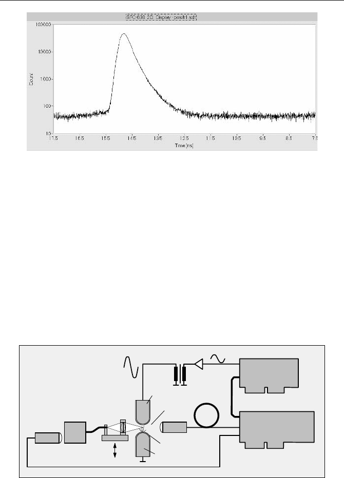
desired positron lifetime distribution. A typical result is shown in Fig. 5.140.

208 5 Application of Modern TCSPC Techniques

Fig. 5.140 Result of a positron lifetime experiment. SPC630 TCSPC Module, XP2020

PMTs . Acquisition time 20 minutes

5.14.5 Diagnostics of Barrier Discharges

The study of barrier discharges (also referred to as dielectric barrier discharges or

silent discharges) is important for understanding mechanisms of degradation and

breakdown of insulators as well as the reactions in the gas of the discharge. A

barrier discharge consists of a large number of microdischarges of nanosecond

duration. The microdischarges appear at random times and random locations over

the surface of an insulator.

The experiment shown in Fig. 5.141 records the shape of the light pulses emitted

by the plasma of single microdischarges in air as a function of the voltage, the wave-

length, and the location in the discharge gap [69, 286, 287, 288, 528, 529, 530].

Stop PMT

Start PMT

Delay

Line

Routing

SYNC

CFD

high voltage

Analog Out

Digital Out

Mono-

chromator

Discharge

Insulator

PPG-100

TCSPC module

sine wave

SPC-530

Electrode

Lens

Fibre

scan

Electrode

Fig. 5.141 Detection of random light pulses from electrical discharges at the surface of an

insulator

The stop signal for the TCSPC measurement is generated by a PMT. The stop

PMT receives the light in a wide spectral range from one side of the discharge

gap. The light pulses are strong enough to release a large number of photoelec-

5.14 Miscellaneous TCSPC Applications 209

trons in the stop PMT. The stop PMT is operated at a gain below the single photon

detection level. It therefore delivers a timing reference signal of relatively low

jitter (see also Fig. 7.44, page 306). The pulses from the stop PMT are delayed and

fed into the stop input of a TCSPC module (SPC

530, Becker & Hickl, Berlin).

The light from the other side of the discharge gap is focused on the input of an

optical fibre and fed into a monochromator. The light of the selected wavelength is

detected by the start PMT. Due to the low numerical aperture and narrow wave-

length interval transmitted by the monochromator, the efficiency in the detection

path is much lower than for the stop PMT. Therefore the start PMT detects single

photons at a rate considerably lower than the average rate of the discharge pulses.

The single-photon pulses are used as start pulses of the TCSPC module and proc-

essed in the ordinary way.

The electrical field in the discharge gap is generated by a high-voltage trans-

former. The transformer is driven by a sine-wave voltage from a digital waveform

generator (PPG

100, Becker & Hickl, Berlin). The waveform generator feeds a

digital equivalent of the sine-wave voltage into the routing input of the TCSPC mod-

ule. When a photon is detected, it is accumulated in a memory block corresponding

to the momentary voltage and in a time channel corresponding to its time referred to

the stop pulse. Therefore the TCSPC modules records the photon distribution over

the voltage across the discharge gap and the time within the discharge duration. A

large number of such distributions are obtained sequentially by scanning the mono-

chromator wavelength or the fibre position along the discharge gap.

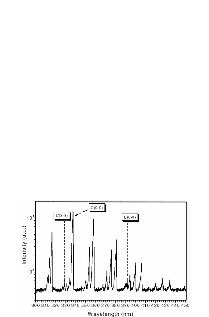
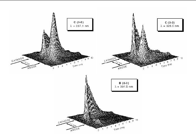
Typical results [288] are shown in Fig. 5.142 and Fig. 5.143. Figure 5.142

shows the time-integrated spectrum of the discharges. The recorded photon distri-

butions over the time in the discharge and the length of the discharge gap are

shown in Fig. 5.143.

Fig. 5.142 Time-integrated spectrum of the barrier discharge in air. The wavelengths used

for time-resolved measurements are indicated. From [288]

210 5 Application of Modern TCSPC Techniques

Fig. 5.143 Time-resolved photon distributions along the discharge gap for the wavelengths

indicated in Fig. 5.142. From [288]

5.14.6 Sonoluminescence

The principle shown in Fig. 5.141 can be applied to a number of similar experi-

ments with randomly emitted light pulses. An early application was the measure-

ment of scintillator decay times by radioactive decay [167] and the use of scintilla-

tion pulses for fluorescence excitation.

A more recent application is time-resolved recording of sonoluminescence.

Sonoluminescence is generated if a gas bubble in a liquid is excited by ultrasound

[20, 72, 139, 190, 233]. The emitted light consists of extremely short flashes with

a duration of 100 ps and less.

For time-resolved detection of the flashes, TCSPC detection systems are used.

The light signal is split into two parts. One part is detected by a stop PMT and

delivers the stop signal to the TCSPC device. The stop PMT works in a mul-

tiphoton mode and thus delivers a low-jitter timing reference. The other part is fed

through a monochromator and detected by the start PMT. The start PMT is oper-

ated in the single photon mode. The TCSPC module records the average shape of

the light pulses.

The efficiency of the measurement can be increased by multiwavelength detec-

tion. The monochromator is replaced with a polychromator, and a multianode

PMT with routing electronics is used to detect the full spectrum. However, despite

its obvious benefits, no application of multiwavelength TCSPC to sonolumines-

cence has yet been published.

5.14 Miscellaneous TCSPC Applications 211

5.14.7 The TCSPC Oscilloscope

If a TCSPC module is operated at a count rate of 10

to 10

photons per second a

reasonably accurate waveform is recorded within less than 100 ms. Advanced

TCSPC modules can therefore be used as optical oscilloscopes. A repetitive meas-

urement cycle is performed in short intervals and the recorded photon distribution

versus time is displayed. Even with a low-cost PMT module, e.g. the Hamamatsu

H5783, an IRF width of about 180 ps is achieved. This corresponds to a signal

bandwidth of almost 2 GHz. The time channel width can be made as short as a

picosecond, which results in an equivalent sample rate of 1,000 GS/s.

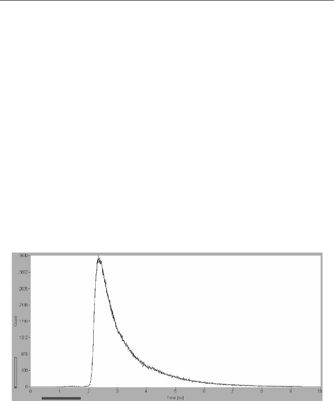
Figure 5.144 shows an example of a TCSPC oscilloscope measurement. The

fluorescence of chlorophyll in a leaf was recorded at a count rate of 4

10

photons

per second and an acquisition time of 100 ms. The time channel width was 9.8 ps.

The fluorescence was excited by a diode laser at a wavelength of 650 nm and a

repetition rate of 50 MHz.

The total cost of a TCSPC oscilloscope system is no higher than that of an opti-

cal oscilloscope consisting of a fast photodiode and a fast oscilloscope. However,

the sensitivity is many orders of magnitude greater. Moreover, the detection area

of a PMT is much larger than that of an ultrafast photodiode, so alignment is no

longer an issue.

Fig. 5.144 Fluorescence signal recorded in an TCSPC oscilloscope setup. One channel of a

Becker & Hickl SPC144, detector count rate 6 MHz, recorded count rate 4 MHz,

1,024 time bins per curve, acquisition time 100 ms per curve. To reproduce the visual im-

pression, two successive traces were overlaid

In practice a stack of filters in front of the PMT is used for convenient

operation under normal daylight conditions. A narrow-band interference filter with

a transmission centred at the wavelength of the detected signal can be added to

reduce the daylight sensitivity.

Convenient detectors for oscilloscope application are the Hamamatsu H5783 or

H5773 modules, or detector heads based on these modules. The modules have a

212 5 Application of Modern TCSPC Techniques

built-in high-voltage generator so that any handling of high voltage is avoided.

This is an important feature for practical use.

Recently fast and relatively inexpensive SPAD modules have become available

[245]. The detectors have an active area of 50 µm diameter and are overload-

proof. The IRF width is about 40 ps, resulting in an equivalent signal bandwidth of

about 9 GHz. Although the small active area can cause some alignment problems,

these detectors are excellently suitable for TCSPC oscilloscopes.

A TCSPC oscilloscope mode is implemented in most advanced TCSPC mod-

ules. The mode has become an indispensable tool for a large number of technical

jobs. Alignment and optimisation of optical systems often requires not only

maximising the efficiency but also localising and removing optical reflections,

leakage of excitation light, or pulse dispersion.

The oscilloscope mode is also used to optimise detectors and the driving condi-

tions of picosecond diode lasers. Another potential application is beam monitoring

in synchrotrons. Furthermore, the oscilloscope mode is a convenient way to opti-

mise TCSPC system parameters, such as signal delay, CFD zero cross and thresh-

old, and TAC parameters.

6 Detectors for Photon Counting

6.1 Detector Principles

6.1.1 Conventional Photomultiplier Tubes

The most frequently used detectors for low-level detection of light are photomul-

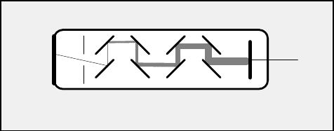
tiplier tubes. A conventional photomultiplier tube (PMT) is a vacuum device that

contains a photocathode, a number of dynodes (amplifying stages) and an anode

that delivers the output signal (Fig. 6.1).

cathode

D2 D3

D6 D7

Anode

Photo-

Dynodes

Fig. 6.1 Functional principle of a conventional photomultiplier tube

The operating voltage builds up an electrical field that accelerates the electrons

from the cathode to the first dynode, D1, from D1 to D2, further from dynode to

dynode, and from the last dynode to the anode. When a photoelectron is emitted at

the photocathode it is accelerated towards the first dynode, D1. When it hits D1 it

releases several secondary electrons. The same happens for the electrons emitted

by D1 when they hit D2. The overall gain reaches values of 10

to 10

. The secon-

dary emission at the dynodes is very fast. In a properly designed dynode system

the secondary electrons resulting from one photoelectron arrive at the anode

within a time interval of a few ns. The resulting current pulse at the anode has a

correspondingly short duration. Due to the high gain and the short output pulse

width, a PMT produces easily detectable current pulses for the individual photons

of a light signal.

A wide variety of photomultipliers are used, with different shapes, different

cathode geometries and diameters, and different dynode geometries [219, 297,

348]. Some tube designs have been successfully used for more than 50 years.

Typical design principles are shown in Fig. 6.2.