Bear H.S. Understanding Calculus
Подождите немного. Документ загружается.

UNDERSTANDING
CALCULUS
Second Edition
IEEEPress
445 Hoes Lane
Piscataway,
NJ 08854
IEEE Press Editorial Board
Stamatios
V.
Kartalopoulos, Editorin Chief
M.Akay
1.
B.Anderson
R.
1.
Baker
1.
E. Brewer
M. E. El-Hawary
R.
1.
Herrick
D.Kirk
R. Leonardi
M. S.Newman
M.Padgett
W.
D. Reeve
S.
Tewksbury
G. Zobrist
Kenneth Moore,
Director
of
Book and Information Services
Catherine
Faduska,
SeniorAcquisitions Editor
Christina
Kuhnen,
AssociateAcquisitions Editor
Technical Reviewers
KemalA. Delic,Hewlett-Packard
Company
ChristieEzeife, University
of
Windsor
HowardHamilton, University
of
Regina
Huan Liu,
Tempe
AZ
Books of Related Interest from the IEEE Press
THE
CALCULUS
TUTORING
BOOK
C. Ash and R.Ash
1993 Softcover 544 pp ISBN 0-7803-1044-6
ONESAND
ZEROS:
Understanding Boolean
Algebra,
Digital
Circuits,
and theLogic
of
Sets
John R. Gregg
1998 Softcover 296 pp ISBN 0-7803-3426-4
THE PROBABILITY
TUTORING
BOOK: Intuitive Essentials for Engineers and Scientists
andEveryoneElse!
CarolAsh
1993 Softcover 480 pp ISBN 0-7803-1051-9
UNDERSTANDING
CALCULUS
Second Edition
H. S.
Bear
Professor Emeritus
Department
of
Mathematics
University
of
Hawaii
IEEE
Press
Understanding Science& Technology Series
+IEEE
IEEE
PRESS
ffiWILEY-
~INTERSCIENCE
A JOHN WILEY & SONS PUBLICATION
Copyright© 2003 byThe Institute of Electricaland ElectronicsEngineers.All rights reserved.
Publishedby John Wiley& Sons, Inc., Hoboken,New
Jersey.
No part of this publicationmay be reproduced, stored in a retrievalsystemor transmittedin any form or
by any means, electronic,mechanical,photocopying, recording, scanningor otherwise,except as
permittedunder Section 107 or 108 of the 1976United States CopyrightAct, without either the prior
written permission of the Publisher, or authorizationthrough payment of the appropriateper-copy fee to
the CopyrightClearance Center,Inc., 222 RosewoodDrive, Danvers,MA 01923, (978) 750-8400,fax
(978) 750-4744,or on the web at www.copyright.com. Requeststo the Publisherfor permission should
be addressedto the PermissionsDepartment,John Wiley
& Sons, Inc., 111 River Street, Hoboken,NJ
07030, (201) 748-6011,fax (201) 748-6008,e-mail: permreq@wiley.com.
Limit of Liability/Disclaimerof Warranty: While the publisher and author haveused their best efforts in
preparingthis book, they make no representationor warranties with respect to the accuracy or
completenessof the contents of this book and specificallydisclaimany implied warranties of
merchantabilityor fitness for a particularpurpose.No warrantymaybe created or extendedby sales
representatives or written sales materials.The advice and strategiescontainedherein may not be suitable
for your situation.Youshould consult with a professionalwhere appropriate.Neither the publishernor
author shall be liablefor any loss of profit or any other commercialdamages, includingbut not limited
to special,incidental,consequential,or other damages.
For general informationon our other productsand services please contact our CustomerCare
Departmentwithin the U.S.at 877-762-2974, outsidethe U.S.at 317-572-3993 or fax 317-572-4002.
Wileyalso publishesits books in a varietyof electronicformats. Some contentthat appears in print,
however,
may not be availablein electronicformat.
Library
of
Congress Cataloging-in-Publication Data is available.
ISBN 0-471-43307-1
Printed in the United States of America.
10 9 8 7 6 5 4 3 2
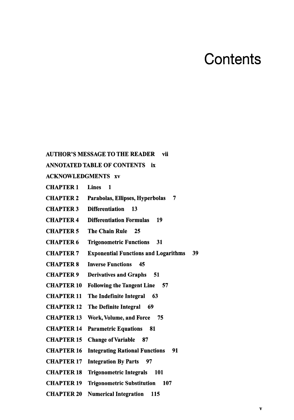
AUTHOR'S MESSAGE TO THE READER vii
ANNOTATED
TABLE OF CONTENTS ix
ACKNOWLEDGMENTS xv
CHAPTER 1 Lines 1
CHAPTER 2 Parabolas, Ellipses,Hyperbolas 7
CHAPTER 3 Differentiation 13
CHAPTER 4 Differentiation Formulas 19
CHAPTER 5 The Chain Rule 25
CHAPTER 6 Trigonometric Functions 31
CHAPTER 7 Exponential Functions and Logarithms 39
CHAPTER 8 Inverse Functions 45
CHAPTER
9 Derivatives and Graphs 51
CHAPTER
10 Following the Tangent Line 57
CHAPTER 11 The Indefinite Integral 63
CHAPTER 12 The Definite Integral 69
CHAPTER 13 Work,Volume, and Force 75
CHAPTER 14 Parametric Equations 81
CHAPTER 15 Change ofVariable 87
CHAPTER 16 Integrating Rational Functions 91
CHAPTER 17 Integration By Parts 97
CHAPTER 18 Trigonometric Integrals 101
CHAPTER 19 Trigonometric Substitution 107
CHAPTER 20 Numerical Integration 115
Contents
v
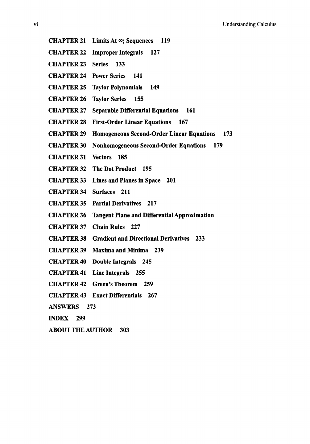
vi Understanding Calculus
CHAPTER 21 Limits At
00;
Sequences 119
CHAPTER 22 Improper Integrals 127
CHAPTER 23 Series 133
CHAPTER 24 Power Series 141
CHAPTER 25 Taylor Polynomials 149
CHAPTER 26 Taylor Series 155
CHAPTER 27 Separable Differential Equations 161
CHAPTER 28 First-Order Linear Equations 167
CHAPTER 29 Homogeneous Second-Order Linear Equations 173
CHAPTER 30
Nonhomogeneous Second-Order Equations 179
CHAPTER 31 Vectors
185
CHAPTER 32 The Dot Product
195
CHAPTER 33 Lines and Planes in Space 201
CHAPTER 34 Surfaces
211
CHAPTER 35 Partial Derivatives 217
CHAPTER 36 Tangent Plane and Differential Approximation
CHAPTER 37 Chain Rules 227
CHAPTER 38 Gradient and Directional Derivatives 233
CHAPTER 39 Maxima and Minima 239
CHAPTER 40 Double Integrals 245
CHAPTER 41 Line Integrals 255
CHAPTER 42 Green's Theorem 259
CHAPTER 43 Exact Differentials 267
ANSWERS 273
INDEX 299
ABOUT THE AUTHOR 303
Author's
Message
to the
Reader
In our earlier book, Understanding Calculus-A UsersGuide, we coveredthe essentials of
one-variable calculus. This book continuesin the same spirit with the treatmentof vectors
and the calculusof severalvariables. In both books our aim is to explainthe materialdirectly
to the reader, in a way which makes sense to a beginning student. This approach is quite
different from that of the usual calculus text. Those books are designed to appeal to the
instructor rather than the student, for it is the.instructorwho chooses the text. Accordingly,
the standard calculus book tries to include every topic that any instructor might want to
cover.
The result is a huge,
heavy,
expensive tome which is better suited for weighttraining
than calculusinstruction.
Most of the techniques of calculus arose as mathematical approaches to concrete
physicalor geometricproblems, and this is the spiritin whichwe approachthe material. The
reader
always
has somethingconcreteto visualize, so usefulintuitioncanbe developed along
with the computational skills. The presentation is never formal, but it is correct. There is
nothingin this book whichwill everhave to be unlearned.
Here is a final, practical observation for students who are currently enrolled in a
standardcalculuscourse. Most instructorsprefer to lecture on theoremsand proofsbecause
that is what a mathematician cares about. Most tests,
however,
will be largely just
problems-problems like those in this book. If you can do the problemsin this book youwill
havelearnedwhat a calculusstudentis supposedto
know.
vii
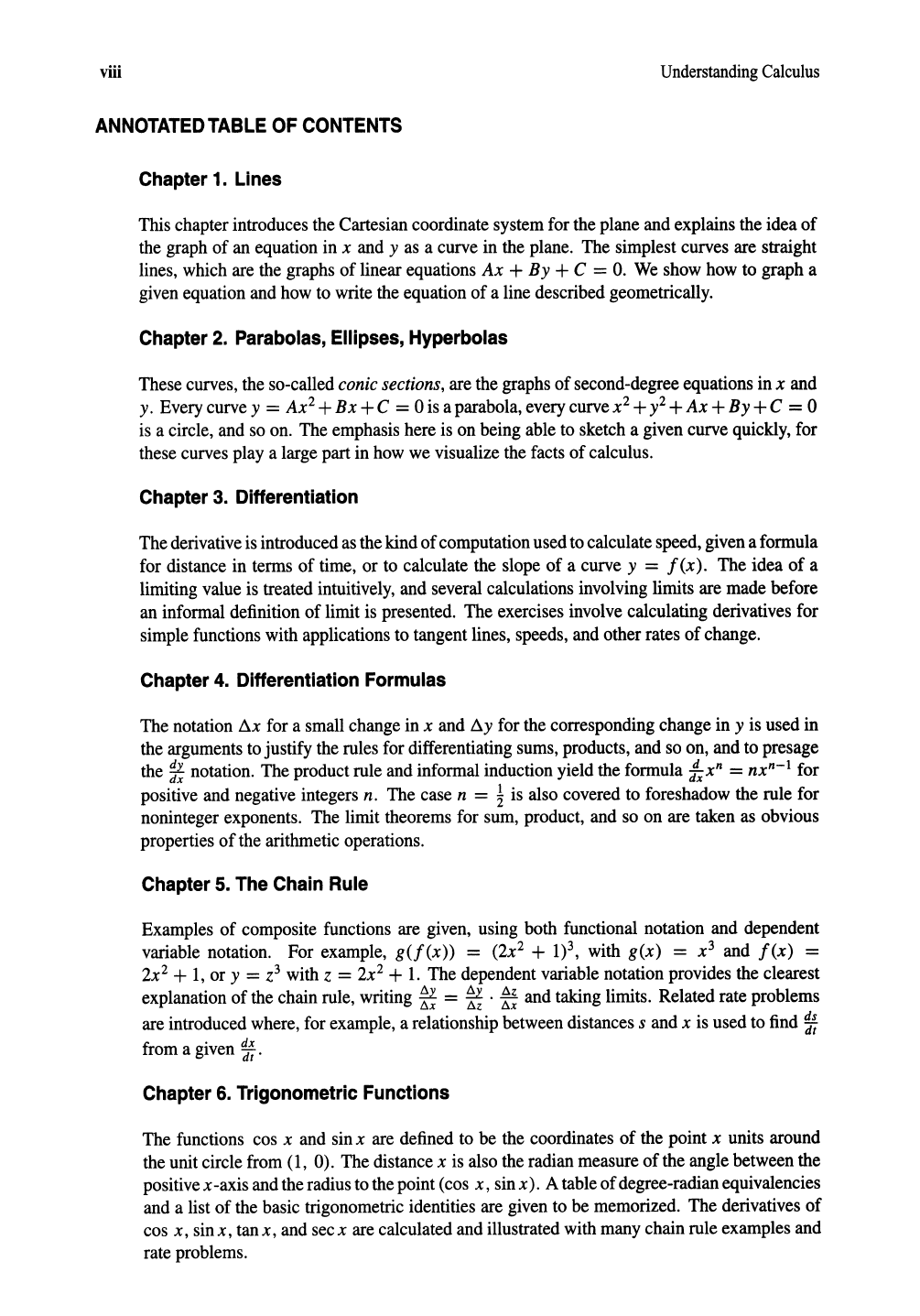
viii
ANNOTATED
TABLE
OF
CONTENTS
Chapter
1.
Lines
Understanding
Calculus
This chapter introduces the Cartesian coordinate system for the plane and explains the idea of
the graph of an equation in
x and y as a curve in the plane. The simplest curves are straight
lines, which are the graphs of linear equations
Ax
+ By + C =
O.
We show how to graph a
given equation and how to write the equation of a line described geometrically.
Chapter
2.
Parabolas,
Ellipses,
Hyperbolas
These curves, the so-called conicsections, are the graphs of second-degree equations in x and
y. Every curve y =
Ax
2
+
Bx
+C =0 is a parabola, every curve x
2
+y2+
Ax
+By +C =0
is a circle, and so on. The emphasis here is on being able to sketch a given curve quickly, for
these curves
playa
large part in how we visualize the facts of calculus.
Chapter
3.
Differentiation
The derivative is introduced as the kind of computation used to calculate speed, given a formula
for distance in terms of time, or to calculate the slope of a curve
y =
f(x).
The idea of a
limiting value is treated intuitively, and several calculations involving limits are made before
an informal definition of limit is presented. The exercises involve calculating derivatives for
simple functions with applications to tangent lines, speeds, and other rates of change.
Chapter
4.
Differentiation
Formulas
The notation
Sx
for a small change in x and
!::J.y
for the corresponding change in y is used in
the arguments to justify the rules for differentiating sums, products, and so on, and to presage
the *notation. The product rule and informal induction yield the formula
fx
x
n
=
nx
n
-
l
for
positive and negative integers
n. The case n = ! is also covered to foreshadow the rule for
noninteger exponents. The limit theorems for sum, product, and so on are taken as obvious
properties
of
the arithmetic operations.
Chapter
5. The
Chain
Rule
Examples of composite functions are given, using both functional notation and dependent
variable notation. For example,
g
(f
(x) = (2x
2
+ 1)3, with g
(x)
= x
3
and f
(x)
=
2x
2
+ 1, or y =Z3 with Z = 2x
2
+ 1. The dependent variable notation provides the clearest
explanation of the chain rule, writing
~
=
~
.
~~
and taking limits. Related rate problems
are introduced where, for example, a relationship between distances
s and x is used to find
~
f
.
dx
rom a gIven dt •
Chapter
6.
Trigonometric
Functions
The functions cos x and sin x are defined to be the coordinates of the point x units around
the unit circle from (1, 0). The distance
x is also the radian measure of the angle between the
positive x -axis and the radius to the point (cos x, sin
x).
A table of degree-radian equivalencies
and a list of the basic trigonometric identities are given to be memorized. The derivatives of
cos
x, sin x, tan x, and sec x are calculated and illustrated with many chain rule examples and
rate problems.
Annotated
Table
of Contents
Chapter
7.
Exponential
Functions
and
Logarithms
ix
The general shape of y = a" for a > 1 is explained, and it is shown that
:x
a" = kaa
x
for some constant k
a
depending on a. We define e to be the number such that k, = 1, so
tx
e" = e", and it is shown that e
==
2.718. The function log x is the inverse of e", and the
derivative
tx
log x =
~
is calculated from the inverse relationship. Many chain rule exercises
involving
eX
and log x are given, as well as some problems involving the exponential growth
of bacteria colonies and compound interest.
Chapter
8.
Inverse
Functions
General inverse functions are defined with
eX
and log x as a convenient example. The nth root
of x, x
~
, is the inverse of x
n
for x >
O.
The derivative of y = x
~
is obtained by differentiating
both sides of
v"
=x, and the chain rule then extends the differentiation formula to fractional
exponents. The functions sin" x, cos" x,
tan-
l
x are defined, and their derivatives are cal-
culated. For example, if y = sin
-1
x, we differentiate both sides of sin y = x and then use
the appropriate right triangle to show that costsin"
x)
=
.JI=X2.
Chapter
9.
Derivatives
and
Graphs
The first and second derivatives are used to determine the shape of a curve. For example,
the function is increasing if
f'(x)
> 0, and concave up if
f"(x)
>
O.
Local maxima and
minima can only occur where
f'(x)
=
O.
Implicit differentiation is used to find the slope
and convexity of a function defined by an equation. Applications are given to curve sketching
and stated max/min problems.
Chapter
10.
Following
the
Tangent
Line
L'Hospital's Rule for limits of the form §is derived quite simply, using the definition of
f'(xo)
and g'(xo) to show that if
f(xo)
= g(xo) = 0, then
~~~
~
'f~~j
as x
~
xo. Newton's
method of solving an equation f (x) = 0 consists of starting with an approximate solution
of
Xl
and following the tangent line back to the x-axis to get the better approximation X2 =
f(xd
Xl
-
f'(xd·
Chapter
11.The Indefinite
Integral
Indefinite integration is the operation inverse to differentiation, so F (x) is the integral or
antiderivative of
f(x)
if
F'(x)
=
f(x).
We start with the problem
oftuming
the gravitational
equation
~ = g into a formula for s in terms of t. All the standard differentiation formulas are
listed alongside the corresponding integration formulas. Some simple differential equations
with initial conditions are solved. The u-substitution is used to explain the backwards use of
the chain rule in integration problems.
Chapter
12. The
Definite
Integral
The area between the curve y =
f(x)
and the x-axis, for a
::::
x
::::
b, is defined to be the limit
of the Riemann sums
L f(Ci)(X; - Xi-I) where the limit is taken as
maxtx,
- Xi-I)
~
O.
This limit is the definite integral, denoted
J:
f (x
)dx.
The Mean Value Theorem shows that
J:
f(x)dx
=
F(b)
-
F(a)
for any antiderivative
F(x)
of
f(x).
Areas between curves are
x Understanding Calculus
calculated using the mnemonic that the area is the sum, indicated by the integral sign, of
vertical "rectangles" of height
f
(x)
and width
dx.
For curves x = f
(y),
one uses horizontal
"rectangles" to get the area in the form
f:
f(y)dy.
Chapter
13.
Work,
Volume,
Force
Work, volume, and force are calculated as integrals that represent limits of sums of increments.
If a force at point
x is f
(x),
then an increment of work done by this force is f (x
)dx,
and the
total work is the sum (integral) of these increments. Similarly, if a solid has cross-sectional
area
A(y)
at height y, then an increment of volume is
A(y)dy,
and total volume is the integral
J
A(y)dy.
Many standard work/volume/force problems are treated.
Chapter
14.
Parametric
Equations
The x and y coordinates of a moving particle are frequently given as functions of t with
equations
y =
f(t),
x =
g(t).
Two such equations are called the parametric equations
of
the path. Many curves are most conveniently described by parametric equations, where the
parameter could be time, or perhaps some variable of geometric importance to the curve. The
~
( 2 )
slope
of
a parametrically given curve is
~
= t, and the concavity
~
is also calculated
in terms of
t. Cauchy's Mean Value Theorem is the ordinary Mean Value Theorem applied to
parametric curves.
Chapter
15.
Change
of
Variable
When a u-substitution is used to change a definite integral in x directly into a definite in-
tegral in u, the process is called a change
of
variable. If the interval of integration for the
original integral is a
~
x
~
b, and u = c when x = a and u = d when x = b, then the
u-integral will have lower limit c and upper limit
d (even if d < c). The new integral formulas
f (a
2
+x
2
( 1
dx
=
~
tan-
1
~
and f (a
2
-
x
2
)
-!
dx
= sin"!
~
are introduced. There are
lots of examples of the technique.
Chapter
16.
Integrating
Rational
Functions
A rational function
~~:~,
where
P(x)
and
Q(x)
are polynomials, can always be integrated
if
Q(x)
can be completely factored. We consider the most common and most useful cases;
namely,
Q(x)
is linear or quadratic, and the degree of
P(x)
is less that the degree of
Q(x).
Chapter
17.
Integration
by
Parts
The integration by parts technique uses the differentiation formula
fx
(u v) =u
~~
+v
~~
in the
integrated form
uv
= J
udv
+J
vdu.
This equation can be used to write one integral in terms
of another: J
udv
= uv - J
vdu.
We cover the principal examples where J
vdu
is simpler
than
J
udv,
and the technique works. Integration by parts is used to integrate log x and the
inverse trigonometric functions.
Chapter
18.
Trigonometric
Integrals
Trigonometric functions are a basic part of scientific language, it is essential to be able to
integrate formulas involving these functions. Trigonometric integrals also arise when substi-
tutions are made to integrate expressions involving radicals. The basic trigonometric identities
