Bayro-Corrochano E., Scheuermann G. Geometric Algebra Computing: in Engineering and Computer Science

Подождите немного. Документ загружается.

8 D. Hestenes

4 Euclidean Geometry with Conformal GA

The conformal model of Euclidean 3-space E

is embedded in the CGA G

4,1

G(R

4,1

) as follows: First, we identify Euclidean points with vectors in the null cone

4,1

≡



x ∈R

4,1

| x



. (17)

Next, we reduce the remaining degrees of freedom from four to three by choosing

a point at inﬁnity e ≡x

∞

and normalizing all points to the hyperplane {x | e · x =

−1,e

=0}.Thus,wehave

∼

4,1

≡



x ∈R

4,1

| x

=0,x·e =−1



. (18)

Finally, we conﬁrm this as a model of Euclidean space by verifying that

−x

=(x

−x

)

=−2x

·x

(19)

correctly determines the Euclidean distance |x

−x

| between any two points. The

argument is completed below.

The amazing fact about this embedding of E

in CGA is that it automatically

imbues all elements of G

4,1

with rich geometric meaning and thereby facilitates

formulation, analysis, and computation in all aspects of Euclidean geometry. It has

two major advantages:

First, it unites the conceptual advantages of classical synthetic geometry with

the analytic power of algebra in providing direct algebraic representations of basic

geometric objects and their properties.

Second, it enlists the apparatus of the conformal versor groups for multiplica-

tive, coordinate- free representation of Euclidean symmetries and transformations.

Speciﬁcally, the invariance group of the Euclidean metric (19)istheEuclidean

group E(3) ={G

}, deﬁned as a subgroup of the conformal group C(3, 0)

∼

O(4, 1)

by the constraint

(e) =G

−1

=e. (20)

This group includes reﬂections. Its restriction to rigid displacements by requiring

=G is the Special Euclidean group SE(3). The rest of this paper is an elabora-

tion of these two points with speciﬁc recommendations for notation, representation,

and method. The subject is young and ﬂuid, so the setting of standards for practice is

still open. Of course, I cannot cover everything. For further details and explanation,

I refer the serious student to [7], which provides the most thorough exposition of

CGA to date, with due emphasis on geometric visualization. Comparison with the

present account shows where I think that exposition can be improved.

In CGA the basic Geometric Objects {O =C,L,S, P } of 3D Euclidean geome-

try can be deﬁned as follows:

• A Circle C is determined by three points:

C =x

∧x

. (21)

New Tools for Computational Geometry 9

• A Line L is a circle through the point at inﬁnity:

L =x

∧x

∧e. (22)

• A Sphere S is determined by four points:

S =x

∧x

. (23)

• A Plane P is a sphere through the point at inﬁnity:

P =x

∧x

∧e. (24)

• A Point x lies on object O if and only if:

x ∧O =0. (25)

Note the distinction between a geometric object O (deﬁned algebraically) and the

set of points O it determines, as expressed by

Line ={x | x ∧L =0}, Plane ={x | x ∧P =0}. (26)

In this respect we follow Euclid in introducing points and lines as distinct objects

with properties speciﬁed by a system of axioms. The idea of deﬁning a line as a set

of points emerged in the 19th century with “containment” replacing the geometric

concept of “incidence” as the basic relation between points and lines. From our

perspective, the limitations of that idea are clear, so we are prepared to use the

concepts of set theory but not to confuse them with concepts of geometry.

Of course our concept of geometric object goes beyond Euclid’s, most notably

in assigning to each an orientation (algebraic sign) and a weight or magnitude (e.g.

length, area, volume). Thus, interchanging the product of points in (21)–(24)re-

verses the sign, hence orientation, of the objects.

For many purposes, the dual representation for a geometric object O

∗

= OI

−1

is most convenient. From the duality of inner an outer products (11) it follows that

the intersection with a point (25) is then expressed by

x ·O

∗

=0. (27)

For a plane, the dual P

∗

=P I

−1

=n is a vector normal to the plane (note the use

of lower-case letters for vectors). The equation x ·n =0 has the familiar form of an

equation for a plane through the origin of a vector space, but in this case it applies

to any plane in E

. For the normal, n speciﬁes a location as well as an orientation

for the plane. Moreover, the separation of E

into disjoint subsets can be neatly

expressed by the inequality x ·n>0 for points in front of the plane, and x ·n<0

for points behind the plane.

The intersection of two planes P

I and P

I is a line speciﬁed by

∗

·P

·(n

I) =(n

∧n

)I. (28)

10 D. Hestenes

Obviously, this vanishes if the planes are parallel. Moreover, as will be evident later,

with the normalization n

=1, the magnitude |n

∧n

| is the sine of the dihe-

dral angle between the intersecting planes.

Similar expressions for the mutual intersections of lines, planes, circles and

spheres are discussed in [7].

5 Invariant Euclidean Geometry

There are two different ways to formulate the equations of spacetime physics: (1) co-

variant formulations expressed with respect to one inertial frame and related to other

frames by Lorentz transformations, and (2) invariant formulations independent of

any reference frame choice. Experts prefer to work with invariants, because they are

invariably simpler than covariants. However, beginners are usually introduced to a

covariant approach, mainly because of educational tradition.

In precise analogy, there are covariant formulations of Euclidean geometry that

depend on designating an arbitrary point as origin, and invariant formulations that

do not. The conformal model supports both approaches, so we should examine their

respective advantages and how they are related.

The characterization of geometric objects in the preceding section is already an

invariant formulation. Let us consider it more closely for extension to an invariant

treatment of any topic in Euclidean geometry. We have seen that CGA supplies

sufﬁcient algebraic structure to deﬁne basic geometric objects. Now note that the

structure of CGA suggests a somewhat different approach to geometric primitives

than the classical one.

The primitive algebraic objects are vectors. In CGA there are four types of vector

with distinct geometric meanings:

Points:



x |x

=0,x·e =−1



Planes:



n | n

> 0,n·e =0



Spheres:



s |s

=±ρ

,s·e =−1



(29)

This suggests that the dual form for a plane n =P

∗

should be regarded as more

fundamental than the 4-vector form in (24). It is also algebraically much more con-

venient, especially for generating translations, as shown below.

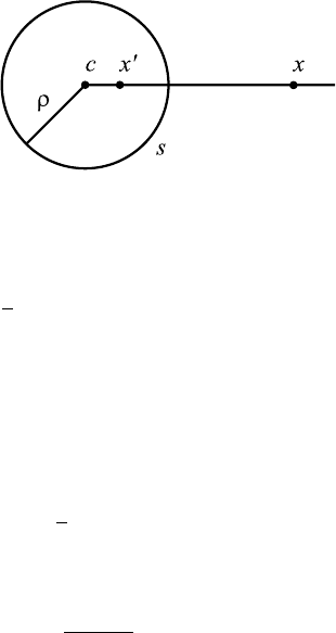
According to (29), there are two types of sphere with radius ρ, corresponding to

the two signs in the square of the sphere vector s. The length of the sphere vector

is scaled so that its square gives the radius directly. The two sphere types are des-

ignated as real and imaginary for positive and negative square respectively. A real

sphere s =S

∗

is the dual of the 4-vector sphere S in (23). It is of interest to note that

the center c of a real sphere can be obtained by a suitably scaled reﬂection from the

point at inﬁnity:

c =−

ses =−

(2e ·s −es)s =s +

e. (30)

New Tools for Computational Geometry 11

Fig. 1

An easy check veriﬁes that c does indeed have the properties of a point. Moreover,

this gives us a natural measure for distance from a point to a sphere:

2s ·x =2



c −



·x =ρ

−|x −c|

. (31)

Thus, the point x is inside, on,oroutside the sphere when s ·x is positive, zero,or

negative respectively. The order is reversed by changing the sign (orientation) of s.

Note that the reﬂection (30) has been deﬁned with respect to the radius of the

sphere instead of unity. This kind of reﬂection is called inversion in a sphere.Ap-

plied to an arbitrary point, it gives a new point,



=−

sxs, (32)

and a little algebra reveals the distance inversion





−c



|x −c|

, (33)

as illustrated in Fig. 1. Though sphere inversion does not preserve Euclidean dis-

tance, it is a powerful means for geometric design and analysis.

The geometric signiﬁcance of imaginary spheres is more subtle, and the reader is

referred to [7] for a discussion. The main point of interest here is that all four vector

types in (29) are needed for computational Euclidean geometry. Subject to scaling,

these constitute all the vectors in the CGA G

4,1

=G(R

4,1

). We can conclude then

that CGA supplies precisely the algebraic structure needed for Euclidean geometry

without anything superﬂuous.

Geometry can be regarded as a system of relations among points. Accordingly,

the most basic is the relation between two points described by the vector n

−x

. This vector is so important that it deserves a name. I like the venerable old

term chord, especially when it is relating points in a geometric ﬁgure or physical

object. Of course, it serves as a displacement vector in other contexts. However,

it has another geometric property unique to CGA; it is the perpendicular bisector

of the interval between the two points. The fact that it is the normal for a plane

is conﬁrmed immediately by n

· e = 0. The fact that it is the bisecting plane is

conﬁrmed from the equation n

·x =0, which as illustrated in Fig. 2, implies (using

(19)) that

|x −x

=−2x ·x

=|x −x

12 D. Hestenes

Fig. 2

Fig. 3

The chords of a triangle are especially signiﬁcant (Fig. 3), for they determine the

basic properties of the Euclidean metric:

−x

≥0.

The chords are related by the triangle equation

=0.

This gives us immediately the familiar law of cosines,

+2n

·n

which determines the basic triangle inequalities for Euclidean distances.

Versor products among the chords generate all the reﬂection and rotation symme-

tries of a triangle and, consequently, values for all the vertex angles. For example,

the versor n

is “complementary” to a rotation “about the vertex x

,” and van-

ishing of its scalar part reduces the law of cosines to the Pythagorean theorem. Note

that the chord n

generates a reﬂection that takes point x

to x

or vise versa. Hence,

the versor product of successive chords generates a walk of reﬂections along any se-

quence of points, which may return to the initial point if the path is closed, as in a

walk around a triangle.

There is much more to be derived from the invariant approach to Euclidean ge-

ometry. For example, according to (21) and (24), the outer product of three vertices

in a triangle determines its circumcircle and the plane in which it lies. Of course,

all this applies to 2D as well as 3D geometry. It would interesting to work out what

insights and simpliﬁcations it brings to the great theorems of classical geometry,

such as the nine circle theorem. Indeed, the results may even have practical value in

applications to mechanical engineering, as we see in later sections.

Finally, to complete our discussion of two point geometry, we note that the sum

e (34)

New Tools for Computational Geometry 13

is a sphere with center c

and poles at the two points. However, in contrast to the

real sphere (30), it is an imaginary sphere. Its role in Euclidean geometry remains

to be worked out.

6 Projective Geometry

Projective geometry is useful in many applications—in computer vision, for

example—but its methodology stands apart from the rest of mathematics. To make

the conceptual assets of projective geometry readily available, we need to incorpo-

rate them into the algebraic design of CGA. As Dieudonné has famously declared,

projective geometry is nothing but linear algebra. Accordingly, let us consider a

generic, nonsingular linear transformation that leaves the point at inﬁnity invariant

(up to a scale factor σ at least):

:x →x



=f (x) with f (e) =σe. (35)

The trouble with this is that it need not preserve the null property of points, so we

have

=0 →



f (x)



(x) ·f (x) =x ·ff(x) =0.

Note: the underbar notation f

denotes a linear operator, while the overbar f denotes

its adjoint. To solve this problem, Anthony Lasenby [12] has proposed that we ex-

tend the notion of points to include planes regarded as boundary points at ∞. Thus,

we extend our model of Euclidean space to include two kinds of points:

interior points:



x |x

=0,x·e =−1



boundary points:



n | n

=1,n·e =0



where the boundary points, like the interior points, are normalized to make them

unique. The set of boundary points can thus be regarded as a Plane (of directions)

at ∞. Indeed, each boundary point can be regarded as the intersection of parallel

lines at ∞, as parallel lines have a common direction. This is an old idea dating

back to Kepler.

Now, projective geometry suppresses metrical notions of scale while maintain-

ing the geometric concept of incidence, as expressed by (28). As that equation re-

quires use of the pseudoscalar and duality, we must extend our notion of projective

transformations to accommodate them. Happily, GA provides a natural way to do

precisely that.

A great advantage of GA is that it enables natural extension of a linear transfor-

mation on vectors to the entire algebra. This extension is called an outermorphism

[5–7, 13] because it preserves the outer product (hence grade), as expressed by

(x ∧M) =f (x) ∧f (M). (36)

14 D. Hestenes

It follows that the pseudoscalar is an eigenblade of the outermorphism, with the

determinant as its eigenvalue:

(I) =(detf )I. (37)

This prepares us for the fundamental theorem [13]:

(detf



∗

·B



=f (A)

∗

·f (B), (38)

which can be made to look more elegant by absorbing (det f

) in A

∗

deﬁned as the

dual with respect to the transformed pseudoscalar (37). This theorem could fairly

be called the Incidence Theorem, because it expresses the fact that outermorphisms

preserve the incidence property (28).

This fundamental theorem of linear algebra has been almost totally overlooked

in the literature, presumably because it is not so naturally expressed in standard

formalisms.

These developments invite us to employ the pseudoscalar to deﬁne “complex

objects” such as

N =x +In, (39)

where x is an interior point, and n is a boundary point. As explained in a later

section, this object can interpreted as a point in a plane if n ·x =0 or, equivalently,

=−1. All this suggests that we should deﬁne projective transformations by

extending outermorphisms to include duality transformations.

I believe that we now have all the necessary ingredients to incorporate projective

geometry smoothly into CGA. There remains the large task of reformulating the

classical results of projective geometry. Since modern works have already formu-

lated many of these results in terms of linear algebra [14], the task should be fairly

straightforward. I recommend it as a good topic for a doctoral thesis.

7 Covariant Euclidean Geometry with Conformal Splits

The most widely used model of Euclidean geometry by far is the vector space model

based on the isomorphism of Euclidean space to a real vector space with Euclidean

inner product:

∼

{x}. (40)

The most effective means of exploiting this model is through its geometric algebra:





={α +a +ib +iβ}, (41)

where i is the unit right-handed pseudoscalar, and the geometric product of vectors

articulates perfectly with the standard dot and cross products:

ab =a ·b +a ∧b =a ·b +ia ×b. (42)

New Tools for Computational Geometry 15

Efﬁcient methods for applying G

to any aspect of mechanics are well developed

with many innovative features [15]. In particular, details of the quaternion theory of

rotations are thoroughly worked out and smoothly articulated with standard vector

methods and matrix representations.

These results even articulate smoothly with the arcane literature on applications

of complex quaternions to geometry and mechanics. For it is evident in (41) that

complex quaternions are isomorphic to multivectors in G

, though practitioners

have not realized that their unit imaginary can be interpreted geometrically as a

pseudoscalar.

Despite all these advantages, the algebra G

suffers from the drawback of all

vector space models, namely, that the vector space (40) singles out the origin as a

preferred point. In other words, it introduces an asymmetry that is not inherent in the

concept of Euclidean space. Happily, that can be remedied by embedding the vector

space model in the conformal model, or better, by factoring it out of the conformal

model. We consider two ways to do that.

The ﬁrst way is a conformal split of CGA into a commuting product of subalge-

bras:

4,1

⊗G

1,1

. (43)

The split is deﬁned geometrically by choosing one point e

as origin and noting

that every other point x lies on the bundle of lines through that point. This deﬁnes a

mapping of points into trivectors:

x =x ∧e

∧e, (44)

which we identify with the vectors in (40). Thus, with a regrading of trivectors as

vectors, we generate G

as a subalgebra of G

4,1

The other subalgebra G

1,1

=G(R

1,1

) in (43) is generated from the null vectors

,e}. Its pseudoscalar is a bivector of sufﬁcient importance to merit a special sym-

bol:

E =e

∧e with E

=(e ·e

)

=1. (45)

We examine this algebra more fully later on. For now, it sufﬁces to note that its con-

tent, though not its structure, depends on the arbitrary choice of the origin point e

It is covariant in the sense that it changes with a change of origin. I have dubbed it

conformal split, because it is deeply analogous to the spacetime split [4, 6], which

is so useful in spacetime physics. The spacetime split is generated by selecting a

timelike vector rather than a null vector as here. Otherwise, the structure and utility

of the splits are quite comparable.

The nature of the conformal split may be clariﬁed by examining a basis for R

4,1

{e, e

} with e

·e

=δ

for j,k =1, 2, 3 and e ·e

=0 =e

·e

. (46)

This generates a basis for R



∧e

∧e =e

∧e) =e

E =Ee



(47)

16 D. Hestenes

and a pseudoscalar

i =σ

=(e

E)(e

E) =e

E =I. (48)

Thus, the pseudoscalar for G

is identical to the pseudoscalar for G

4,1

.Itisan

invariant of the conformal split!

An alternative to the conformal split is the additive split:

4,1



⊕R

1,1



≡G

⊕G

1,1

, (49)

deﬁned by choosing {e

} from (46) as a basis for R

. Unlike the basis (47),

the basis in this case is not algebraically associated with lines through a point, and

the pseudoscalar I

=IE is not an invariant. Furthermore, the σ

commute

with e, while the e

do not. Consequently, the additive split is not as convenient as

the conformal split. Even so, it has its place, most notably in modeling a rigid body,

as we shall see.

To demonstrate the felicity of the conformal split for relating invariant forms for

geometric objects to standard vector space forms, results for the most basic geomet-

ric objects (point, line, plane) are given here.

The mapping (44) of point x to vector x =x ∧E can be inverted. The slickest

way to do that is to use the geometric product thus:

xE =x ∧E +x ·E with x ·E =x ·(e

∧e) =(x ·e

)e +e

. (50)

Multiplying the ﬁrst equation by its reverse, we get

0 =(x ∧E)

−(x ·E)

; whence x

=(x ·E)

=−2x ·e

. (51)

Inserting this back into (50),wesolvetoget

x =



x −

e +e



E =E



x +

e −e



=xE +

e +e

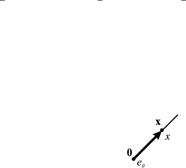
. (52)

This can be regarded as the conformal split of point x with respect to point e

Illustrations of the two representations for points are superimposed in Fig. 4, which

may be misleading because the points are related by projection.

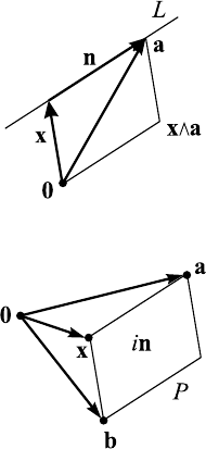
The conformal split of a line L through points x and a gives

L =x ∧a ∧e =x ∧ae +(a −x) =(de +1)n. (53)

Fig. 4

New Tools for Computational Geometry 17

Fig. 5

Fig. 6

Note that this represents the line in terms of its Plücker coordinates, which consists

of a vector, bivector pair for the line tangent, and moment with respect to the origin

(Fig. 5):

tangent: n =a −x, (54)

moment: x ∧a =x ∧(a −x) =dn. (55)

The directed distance from origin to line is given by the directance:

d =(x ∧a)n

−1

=(x ∧n)n

−1

=x −



x ·n

−1



n. (56)

The conformal split of a plane P through points x, a, b gives

P = x ∧a ∧b ∧e =x ∧a ∧b e +(a −x) ∧(b −x)E. (57)

Its Plücker coordinates consists of the bivector–trivector pair (Fig. 6):

tangent: (a −x) ∧(b −x) =x ∧a +a ∧b +b ∧x =in, (58)

moment: x ∧a ∧b =x ∧



(a −x) ∧(b −x)



=x ∧(in) =i(x ·n). (59)

The

dual form for the plane is:

P = i(xne +nE) =in. (60)