Banner A. The Calculus Lifesaver: All the Tools You Need to Excel at Calculus
Подождите немного. Документ загружается.


596 • Complex Numbers
x
2
+ 1 after all—but they are not real: they are imaginary. How about 2i?
That’s also imaginary. In fact, (2i)
2
= 2
2
i
2
= 4(−1) = −4, so (2i)
2
is a
negative number. So, when we say that a number is imaginary, we mean that
its square is a negative number. The only imaginary numbers are of the form
yi where y is a real number not equal to 0. You can also write iy instead of
yi.
Now, you can add or subtract real and imaginary numbers, for example
2 − 3i, but you can’t simplify the result. In this way, we get all the complex
numbers, which are all the numbers of the form x+iy, where x and y are real.
The set of all complex numbers is normally denoted by the symbol C. Notice
that all imaginary numbers are complex numbers; for example, 2i = 0 + 2i.
All real numbers are also complex numbers; for example, −13 = −13 + 0i.
Every complex number has a real and an imaginary part. If z = x + iy, then
the real part is x and the imaginary part is y. These are written as Re(z) and
Im(z), respectively. For example, Re(2 − 3i) = 2 and Im(2 − 3i) = −3. Note
that Im(2 − 3i) is not −3i, it’s just −3. What is Re(2i)? Well, write 2i as
0 + 2i to see that the real part is 0. On the other hand, the imaginary part,
Im(2i), is of course 2.
Adding and subtracting complex numbers is pretty easy. Just add (or
subtract) the real parts, and then do the imaginary parts. For example,
PSfrag
replacements
(
a, b)
[
a, b]
(
a, b]
[
a, b)
(
a, ∞)
[
a, ∞)
(
−∞, b)
(
−∞, b]
(
−∞, ∞)
{
x : a < x < b}
{
x : a ≤ x ≤ b}
{
x : a < x ≤ b}
{
x : a ≤ x < b}
{
x : x ≥ a}
{
x : x > a}
{
x : x ≤ b}
{
x : x < b}
R
a
b
shado
w
0
1
4
−
2
3
−
3
g(
x) = x
2
f(
x) = x
3
g(
x) = x
2
f(
x) = x
3
mirror
(y = x)
f
−
1
(x) =
3
√
x
y = h
(x)
y = h
−
1
(x)
y =
(x − 1)
2
−
1
x
Same
height
−
x
Same
length,
opp
osite signs
y = −
2x
−
2
1
y =
1
2
x − 1
2
−
1
y =
2
x
y =
10
x
y =
2
−x
y =
log
2
(x)
4
3
units
mirror
(x-axis)
y = |
x|
y = |
log
2
(x)|
θ radians
θ units
30
◦
=
π
6
45
◦
=
π
4
60
◦
=
π
3
120
◦
=
2
π
3
135
◦
=
3
π
4
150
◦
=
5
π
6
90
◦
=
π
2
180
◦
= π
210
◦
=
7
π
6
225
◦
=
5
π
4
240
◦
=
4
π
3
270
◦
=
3
π
2
300
◦
=
5
π
3
315
◦
=
7
π
4
330
◦
=
11
π
6
0
◦
=
0 radians
θ
hyp
otenuse
opp
osite
adjacen
t
0
(≡ 2π)
π
2
π
3
π
2
I
I
I
I
II
IV
θ
(
x, y)
x
y
r
7
π
6
reference
angle
reference
angle =
π
6
sin
+
sin −
cos
+
cos −
tan
+
tan −
A
S
T
C
7
π
4
9
π
13
5
π
6
(this
angle is
5π
6
clo
ckwise)
1
2
1
2
3
4
5
6
0
−
1
−
2
−
3
−
4
−
5
−
6
−
3π
−
5
π
2
−
2π
−
3
π
2
−
π
−
π
2
3
π
3
π
5
π
2
2
π
3
π
2
π
π
2
y =
sin(x)
1
0
−
1
−
3π
−
5
π
2
−
2π
−
3
π
2
−
π
−
π
2
3
π
5
π
2
2
π
2
π
3
π
2
π
π
2
y =
sin(x)
y =
cos(x)
−
π
2
π
2
y =
tan(x), −
π
2
<
x <
π
2
0
−
π
2
π
2
y =
tan(x)
−
2π
−
3π
−
5
π
2
−
3
π
2
−
π
−
π
2
π
2
3
π
3
π
5
π
2
2
π
3
π
2
π
y =
sec(x)
y =
csc(x)
y =
cot(x)
y = f(
x)
−
1
1
2
y = g(
x)
3
y = h
(x)
4
5
−
2
f(
x) =
1
x
g(
x) =
1
x
2
etc.
0
1
π
1
2
π
1
3
π
1
4
π
1
5
π
1
6
π
1
7
π
g(
x) = sin
1
x
1
0
−
1
L
10
100
200
y =
π
2
y = −
π
2
y =
tan
−1
(x)
π
2
π
y =
sin(
x)
x
,
x > 3
0
1
−
1
a
L
f(
x) = x sin (1/x)
(0 <
x < 0.3)
h
(x) = x
g(
x) = −x
a
L
lim
x
→a
+
f(x) = L
lim
x
→a
+
f(x) = ∞
lim
x
→a
+
f(x) = −∞
lim
x
→a
+
f(x) DNE
lim
x
→a
−
f(x) = L
lim
x
→a
−
f(x) = ∞
lim
x
→a
−
f(x) = −∞
lim
x
→a
−
f(x) DNE
M
}
lim
x
→a
−
f(x) = M
lim
x
→a
f(x) = L
lim
x
→a
f(x) DNE
lim
x
→∞
f(x) = L
lim
x
→∞
f(x) = ∞
lim
x
→∞
f(x) = −∞
lim
x
→∞
f(x) DNE
lim
x
→−∞
f(x) = L
lim
x
→−∞
f(x) = ∞
lim
x
→−∞
f(x) = −∞
lim
x
→−∞
f(x) DNE
lim
x →a
+
f(
x) = ∞
lim
x →a
+
f(
x) = −∞
lim
x →a
−
f(
x) = ∞
lim
x →a
−
f(
x) = −∞
lim
x →a
f(
x) = ∞
lim
x →a
f(
x) = −∞
lim
x →a
f(
x) DNE
y = f (
x)
a
y =
|
x|
x
1
−
1
y =
|
x + 2|
x +
2
1
−
1
−
2
1
2
3
4
a
a
b
y = x sin
1
x
y = x
y = −
x
a
b
c
d
C
a
b
c
d
−
1
0
1
2
3
time
y
t
u
(
t, f(t))
(
u, f(u))
time
y
t
u
y
x
(
x, f(x))
y = |
x|
(
z, f(z))
z
y = f(
x)
a
tangen
t at x = a
b
tangen
t at x = b
c
tangen
t at x = c
y = x
2
tangen
t
at x = −
1
u
v
uv
u +
∆u
v +
∆v
(
u + ∆u)(v + ∆v)
∆
u
∆
v
u
∆v
v∆
u
∆
u∆v
y = f(
x)
1
2
−
2
y = |
x
2
− 4|
y = x
2
− 4
y = −
2x + 5
y = g(
x)
1
2
3
4
5
6
7
8
9
0
−
1
−
2
−
3
−
4
−
5
−
6
y = f (
x)
3
−
3
3
−
3
0
−
1
2
easy
hard
flat
y = f
0
(
x)
3
−
3
0
−
1
2
1
−
1
y =
sin(x)
y = x
x
A
B
O
1
C
D
sin(
x)
tan(
x)
y =
sin(
x)
x
π
2
π
1
−
1
x =
0
a =
0
x
> 0
a
> 0
x
< 0
a
< 0
rest
position
+
−
y = x
2
sin
1
x
N
A
B
H
a
b
c
O
H
A
B
C
D
h
r
R
θ
1000
2000
α
β
p
h
y = g(
x) = log
b
(x)
y = f(
x) = b
x
y = e
x
5
10
1
2
3
4
0
−
1
−
2
−
3
−
4
y =
ln(x)
y =
cosh(x)
y =
sinh(x)
y =
tanh(x)
y =
sech(x)
y =
csch(x)
y =
coth(x)
1
−
1
y = f(
x)
original
function
in
verse function
slop
e = 0 at (x, y)
slop
e is infinite at (y, x)
−
108
2
5
1
2
1
2
3
4
5
6
0
−
1
−
2
−
3
−
4
−
5
−
6
−
3π
−
5
π
2
−
2π
−
3
π
2
−
π
−
π
2
3
π
3
π
5
π
2
2
π
3
π
2
π
π
2
y =
sin(x)
1
0
−
1
−
3π
−
5
π
2
−
2π
−
3
π
2
−
π
−
π
2
3
π
5
π
2
2
π
2
π
3
π
2
π
π
2
y =
sin(x)
y =
sin(x), −
π
2
≤ x ≤
π
2
−
2
−
1
0
2
π
2
−
π
2
y =
sin
−1
(x)
y =
cos(x)
π
π
2
y =
cos
−1
(x)
−
π
2
1
x
α
β
y =
tan(x)
y =
tan(x)
1
y =
tan
−1
(x)
y =
sec(x)
y =
sec
−1
(x)
y =
csc
−1
(x)
y =
cot
−1
(x)
1
y =
cosh
−1
(x)
y =
sinh
−1
(x)
y =
tanh
−1
(x)
y =
sech
−1
(x)
y =
csch
−1
(x)
y =
coth
−1
(x)
(0
, 3)
(2
, −1)
(5
, 2)
(7
, 0)
(
−1, 44)
(0
, 1)
(1
, −12)
(2
, 305)
y =
1
2
(2
, 3)
y = f(
x)
y = g(
x)
a
b
c
a
b
c
s
c
0
c
1
(
a, f(a))
(
b, f(b))
1
2
1
2
3
4
5
6
0
−
1
−
2
−
3
−
4
−
5
−
6
−
3π
−
5
π
2
−
2π
−
3
π
2
−
π
−
π
2
3
π
3
π
5
π
2
2
π
3
π
2
π
π
2
y =
sin(x)
1
0
−
1
−
3π
−
5
π
2
−
2π
−
3
π
2
−
π
−
π
2
3
π
5
π
2
2
π
2
π
3
π
2
π
π
2
c
OR
Lo
cal maximum
Lo
cal minimum
Horizon
tal point of inflection
1
e
y = f
0
(
x)
y = f (
x) = x ln(x)
−
1
e
?
y = f(
x) = x
3
y = g(
x) = x
4
x
f(
x)
−
3
−
2
−
1
0
1
2
1
2
3
4
+
−
?
1
5
6
3
f
0
(
x)
2 −
1
2
√
6
2
+
1
2
√
6
f
00
(
x)
7
8
g
00
(
x)
f
00
(
x)
0
y =
(
x − 3)(x − 1)
2
x
3
(
x + 2)
y = x ln
(x)
1
e
−
1
e
5
−
108
2
α
β
2 −
1
2
√
6
2
+
1
2
√
6
y = x
2
(
x − 5)
3
−
e
−
1/2
√
3
e
−
1/2
√
3
−
e
−3/2
e
−
3/2
−
1
√
3
1
√
3
−
1
1
y = xe
−
3x
2
/2
y =
x
3
− 6
x
2
+ 13x − 8
x
28
2
600
500
400
300
200
100
0
−
100
−
200
−
300
−
400
−
500
−
600
0
10
−
10
5
−
5
20
−
20
15
−
15
0
4
5
6
x
P
0
(
x)
+
−
−
existing
fence
new
fence
enclosure
A
h
b
H
99
100
101
h
dA/dh
r
h
1
2
7
shallo
w
deep
LAND
SEA
N
y
z
s
t
3
11
9
L
(11)
√
11
y = L
(x)
y = f (
x)
11
y = L
(x)
y = f(
x)
F
P
a
a +
∆x
f(
a + ∆x)
L
(a + ∆x)
f(
a)
error
d
f
∆
x
a
b
y = f(
x)
true
zero
starting
approximation
b
etter approximation
v
t
3
5
50
40
60
4
20
30
25
t
1
t
2
t
3
t
4
t
n
−2
t
n
−1
t
0
= a
t
n
= b
v
1
v
2
v
3
v
4
v
n
−1
v
n
−
30
6
30
|
v|
a
b
p
q
c
v(
c)
v(
c
1
)
v(
c
2
)
v(
c
3
)
v(
c
4
)
v(
c
5
)
v(
c
6
)
t
1
t
2
t
3
t
4
t
5
c
1
c
2
c
3
c
4
c
5
c
6
t
0
=
a
t
6
=
b
t
16
=
b
t
10
=
b
a
b
x
y
y = f(
x)
1
2
y = x
5
0
−
2
y =
1
a
b
y =
sin(x)
π
−
π
0
−
1
−
2
0
2
4
y = x
2
0
1
2
3
4
2
n
4
n
6
n
2(
n−2)
n
2(
n−1)
n
2
n
n
=
2
width
of each interval =
2
n
−
2
1
3
0
I
I
I
I
II
IV
4
y
dx
y = −
x
2
− 2x + 3
3
−
5
y = |−
x
2
− 2x + 3|
I
I
I
I
Ia
5
3
0
1
2
a
b
y = f (
x)
y = g(
x)
y = x
2
a
b
5
3
0
1
2
y =
√
x
2
√
2
2
2
dy
x
2
a
b
y = f(
x)
y = g(
x)
M
m
1
2
−
1
−
2
0
y = e
−
x
2
1
2
e
−
1/4
f
a
v
y = f
a
v
c
A
M
0
1
2
a
b
x
t
y = f (
t)
F (
x )
y = f (
t)
F (
x + h)
x + h
F (
x + h) − F (x)
f(
x)
1
2
y =
sin(x)
π
−
π
−
1
−
2
y =
1
x
y = x
2
1
2
1
−
1
y =
ln|x|
θ
a
x
a
x
p
a
2
− x
2
3
x
p
9 − x
2
p
x
2
+ a
2
x
a
p
x
2
+ 15
x
√
15
x
p
x
2
− a
2
a
x
p
x
2
− 4
2
x
−
p
x
2
− a
2
a
x
−
p
x
2
− 4
2
y = f(
x)
a
b
a + ε
ε
Z
b
a
+ε
f(x) dx
small
ev
en smaller
y = g(
x)
infinite
area
finite
area
1
y =
1
x
y =
1
x
p
, p
< 1 (typical)
y =
1
x
p
, p
> 1 (typical)
a
1
a
2
a
3
a
4
a
5
a
6
a
7
a
8
1
2
3
4
5
6
7
8
n
a
n
x
y
y = f(
x)
(
a, f(a))
a
−
1
0
1
a
6
1
2
7
1
2
7
?
−
2
−
1
−
2
t =
0
t = π
/6
t = π
/4
t = π
/3
t = π
/2
3
0
t = −
2
t = −3/2
t = ±1
t = −1/2
t = 0
t = 1/2
t = 3/2
t = 2
12
−12
θ
r
P
θ
r
P
11π
6
2
(−1, −1)
wrong point
π
4
5π
4
√
2
(0, 1)
(0, −3)
(−2, 0)
π
2
3π
2
π
r = 3 sin(θ)
3π
2
θ
2π
1
0
−1
−2
−3
0
3
2
−
3
2
0
r = 1 + 2 cos(θ)
2π
3
4π
3
0
π
0
pi
−
3
2
3π
2
1
2
3
0
−1
−2
−3
0 ≤ θ ≤
2π
3
0 ≤ θ ≤ π
0 ≤ θ ≤ 2π
r = 1 + cos(θ)
r = 1 +
3
4
cos(θ)
−
1
4
r = sin(2θ)
r = sin(3θ)
r =
1
π
θ
0 ≤ θ ≤ 4π
r =
2
1 + sin(θ)
−
π
4
≤ θ ≤
5π
4
0 ≤ θ ≤ 2π
0 ≤ θ ≤ π
−4
−5
4
5
f(θ)
f(θ + dθ)
θ
dθ
θ + dθ
approximating region
exact region
0 ≤ θ ≤ 2π
r = |1 + 2 cos(θ)|
(2 − 3i) + (−6 − 7i) = 2 − 6 − 3i − 7i = −4 − 10i;
an example of subtraction is
PSfrag
replacements
(
a, b)
[
a, b]
(
a, b]
[
a, b)
(
a, ∞)
[
a, ∞)
(
−∞, b)
(
−∞, b]
(
−∞, ∞)
{
x : a < x < b}
{
x : a ≤ x ≤ b}
{
x : a < x ≤ b}
{
x : a ≤ x < b}
{
x : x ≥ a}
{
x : x > a}
{
x : x ≤ b}
{
x : x < b}
R
a
b
shado
w
0
1
4
−
2
3
−
3
g(
x) = x
2
f(
x) = x
3
g(
x) = x
2
f(
x) = x
3
mirror
(y = x)
f
−
1
(x) =
3
√
x
y = h
(x)
y = h
−
1
(x)
y =
(x − 1)
2
−
1
x
Same
height
−
x
Same
length,
opp
osite signs
y = −
2x
−
2
1
y =
1
2
x − 1
2
−
1
y =
2
x
y =
10
x
y =
2
−x
y =
log
2
(x)
4
3
units
mirror
(x-axis)
y = |
x|
y = |
log
2
(x)|
θ radians
θ units
30
◦
=
π
6
45
◦
=
π
4
60
◦
=
π
3
120
◦
=
2
π
3
135
◦
=
3
π
4
150
◦
=
5
π
6
90
◦
=
π
2
180
◦
= π
210
◦
=
7
π
6
225
◦
=
5
π
4
240
◦
=
4
π
3
270
◦
=
3
π
2
300
◦
=
5
π
3
315
◦
=
7
π
4
330
◦
=
11
π
6
0
◦
=
0 radians
θ
hyp
otenuse
opp
osite
adjacen
t
0
(≡ 2π)
π
2
π
3
π
2
I
I
I
I
II
IV
θ
(
x, y)
x
y
r
7
π
6
reference
angle
reference
angle =
π
6
sin
+
sin −
cos
+
cos −
tan
+
tan −
A
S
T
C
7
π
4
9
π
13
5
π
6
(this
angle is
5π
6
clo
ckwise)
1
2
1
2
3
4
5
6
0
−
1
−
2
−
3
−
4
−
5
−
6
−
3π
−
5
π
2
−
2π
−
3
π
2
−
π
−
π
2
3
π
3
π
5
π
2
2
π
3
π
2
π
π
2
y =
sin(x)
1
0
−
1
−
3π
−
5
π
2
−
2π
−
3
π
2
−
π
−
π
2
3
π
5
π
2
2
π
2
π
3
π
2
π
π
2
y =
sin(x)
y =
cos(x)
−
π
2
π
2
y =
tan(x), −
π
2
<
x <
π
2
0
−
π
2
π
2
y =
tan(x)
−
2π
−
3π
−
5
π
2
−
3
π
2
−
π
−
π
2
π
2
3
π
3
π
5
π
2
2
π
3
π
2
π
y =
sec(x)
y =
csc(x)
y =
cot(x)
y = f(
x)
−
1
1
2
y = g(
x)
3
y = h
(x)
4
5
−
2
f(
x) =
1
x
g(
x) =
1
x
2
etc.
0
1
π
1
2
π
1
3
π
1
4
π
1
5
π
1
6
π
1
7
π
g(
x) = sin
1
x
1
0
−
1
L
10
100
200
y =
π
2
y = −
π
2
y =
tan
−1
(x)
π
2
π
y =
sin(
x)
x
,
x > 3
0
1
−
1
a
L
f(
x) = x sin (1/x)
(0 <
x < 0.3)
h
(x) = x
g(
x) = −x
a
L
lim
x
→a
+
f(x) = L
lim
x
→a
+
f(x) = ∞
lim
x
→a
+
f(x) = −∞
lim
x
→a
+
f(x) DNE
lim
x
→a
−
f(x) = L
lim
x
→a
−
f(x) = ∞
lim
x
→a
−
f(x) = −∞
lim
x
→a
−
f(x) DNE
M
}
lim
x
→a
−
f(x) = M
lim
x
→a
f(x) = L
lim
x
→a
f(x) DNE
lim
x
→∞
f(x) = L
lim
x
→∞
f(x) = ∞
lim
x
→∞
f(x) = −∞
lim
x
→∞
f(x) DNE
lim
x
→−∞
f(x) = L
lim
x
→−∞
f(x) = ∞
lim
x
→−∞
f(x) = −∞
lim
x
→−∞
f(x) DNE
lim
x →a
+
f(
x) = ∞
lim
x →a
+
f(
x) = −∞
lim
x →a
−
f(
x) = ∞
lim
x →a
−
f(
x) = −∞
lim
x →a
f(
x) = ∞
lim
x →a
f(
x) = −∞
lim
x →a
f(
x) DNE
y = f (
x)
a
y =
|
x|
x
1
−
1
y =
|
x + 2|
x +
2
1
−
1
−
2
1
2
3
4
a
a
b
y = x sin
1
x
y = x
y = −
x
a
b
c
d
C
a
b
c
d
−
1
0
1
2
3
time
y
t
u
(
t, f(t))
(
u, f(u))
time
y
t
u
y
x
(
x, f(x))
y = |
x|
(
z, f(z))
z
y = f(
x)
a
tangen
t at x = a
b
tangen
t at x = b
c
tangen
t at x = c
y = x
2
tangen
t
at x = −
1
u
v
uv
u +
∆u
v +
∆v
(
u + ∆u)(v + ∆v)
∆
u
∆
v
u
∆v
v∆
u
∆
u∆v
y = f(
x)
1
2
−
2
y = |
x
2
− 4|
y = x
2
− 4
y = −
2x + 5
y = g(
x)
1
2
3
4
5
6
7
8
9
0
−
1
−
2
−
3
−
4
−
5
−
6
y = f (
x)
3
−
3
3
−
3
0
−
1
2
easy
hard
flat
y = f
0
(
x)
3
−
3
0
−
1
2
1
−
1
y =
sin(x)
y = x
x
A
B
O
1
C
D
sin(
x)
tan(
x)
y =
sin(
x)
x
π
2
π
1
−
1
x =
0
a =
0
x
> 0
a
> 0
x
< 0
a
< 0
rest
position
+
−
y = x
2
sin
1
x
N
A
B
H
a
b
c
O
H
A
B
C
D
h
r
R
θ
1000
2000
α
β
p
h
y = g(
x) = log
b
(x)
y = f(
x) = b
x
y = e
x
5
10
1
2
3
4
0
−
1
−
2
−
3
−
4
y =
ln(x)
y =
cosh(x)
y =
sinh(x)
y =
tanh(x)
y =
sech(x)
y =
csch(x)
y =
coth(x)
1
−
1
y = f(
x)
original
function
in
verse function
slop
e = 0 at (x, y)
slop
e is infinite at (y, x)
−
108
2
5
1
2
1
2
3
4
5
6
0
−
1
−
2
−
3
−
4
−
5
−
6
−
3π
−
5
π
2
−
2π
−
3
π
2
−
π
−
π
2
3
π
3
π
5
π
2
2
π
3
π
2
π
π
2
y =
sin(x)
1
0
−
1
−
3π
−
5
π
2
−
2π
−
3
π
2
−
π
−
π
2
3
π
5
π
2
2
π
2
π
3
π
2
π
π
2
y =
sin(x)
y =
sin(x), −
π
2
≤ x ≤
π
2
−
2
−
1
0
2
π
2
−
π
2
y =
sin
−1
(x)
y =
cos(x)
π
π
2
y =
cos
−1
(x)
−
π
2
1
x
α
β
y =
tan(x)
y =
tan(x)
1
y =
tan
−1
(x)
y =
sec(x)
y =
sec
−1
(x)
y =
csc
−1
(x)
y =
cot
−1
(x)
1
y =
cosh
−1
(x)
y =
sinh
−1
(x)
y =
tanh
−1
(x)
y =
sech
−1
(x)
y =
csch
−1
(x)
y =
coth
−1
(x)
(0
, 3)
(2
, −1)
(5
, 2)
(7
, 0)
(
−1, 44)
(0
, 1)
(1
, −12)
(2
, 305)
y =
1
2
(2
, 3)
y = f(
x)
y = g(
x)
a
b
c
a
b
c
s
c
0
c
1
(
a, f(a))
(
b, f(b))
1
2
1
2
3
4
5
6
0
−
1
−
2
−
3
−
4
−
5
−
6
−
3π
−
5
π
2
−
2π
−
3
π
2
−
π
−
π
2
3
π
3
π
5
π
2
2
π
3
π
2
π
π
2
y =
sin(x)
1
0
−
1
−
3π
−
5
π
2
−
2π
−
3
π
2
−
π
−
π
2
3
π
5
π
2
2
π
2
π
3
π
2
π
π
2
c
OR
Lo
cal maximum
Lo
cal minimum
Horizon
tal point of inflection
1
e
y = f
0
(
x)
y = f (
x) = x ln(x)
−
1
e
?
y = f(
x) = x
3
y = g(
x) = x
4
x
f(
x)
−
3
−
2
−
1
0
1
2
1
2
3
4
+
−
?
1
5
6
3
f
0
(
x)
2 −
1
2
√
6
2
+
1
2
√
6
f
00
(
x)
7
8
g
00
(
x)
f
00
(
x)
0
y =
(
x − 3)(x − 1)
2
x
3
(
x + 2)
y = x ln
(x)
1
e
−
1
e
5
−
108
2
α
β
2 −
1
2
√
6
2
+
1
2
√
6
y = x
2
(
x − 5)
3
−
e
−
1/2
√
3
e
−
1/2
√
3
−
e
−3/2
e
−
3/2
−
1
√
3
1
√
3
−
1
1
y = xe
−
3x
2
/2
y =
x
3
− 6
x
2
+ 13x − 8
x
28
2
600
500
400
300
200
100
0
−
100
−
200
−
300
−
400
−
500
−
600
0
10
−
10
5
−
5
20
−
20
15
−
15
0
4
5
6
x
P
0
(
x)
+
−
−
existing
fence
new
fence
enclosure
A
h
b
H
99
100
101
h
dA/dh
r
h
1
2
7
shallo
w
deep
LAND
SEA
N
y
z
s
t
3
11
9
L
(11)
√
11
y = L
(x)
y = f (
x)
11
y = L
(x)
y = f(
x)
F
P
a
a +
∆x
f(
a + ∆x)
L
(a + ∆x)
f(
a)
error
d
f
∆
x
a
b
y = f(
x)
true
zero
starting
approximation
b
etter approximation
v
t
3
5
50
40
60
4
20
30
25
t
1
t
2
t
3
t
4
t
n
−2
t
n
−1
t
0
= a
t
n
= b
v
1
v
2
v
3
v
4
v
n
−1
v
n
−
30
6
30
|
v|
a
b
p
q
c
v(
c)
v(
c
1
)
v(
c
2
)
v(
c
3
)
v(
c
4
)
v(
c
5
)
v(
c
6
)
t
1
t
2
t
3
t
4
t
5
c
1
c
2
c
3
c
4
c
5
c
6
t
0
=
a
t
6
=
b
t
16
=
b
t
10
=
b
a
b
x
y
y = f(
x)
1
2
y = x
5
0
−
2
y =
1
a
b
y =
sin(x)
π
−
π
0
−
1
−
2
0
2
4
y = x
2
0
1
2
3
4
2
n
4
n
6
n
2(
n−2)
n
2(
n−1)
n
2
n
n
=
2
width
of each interval =
2
n
−
2
1
3
0
I
I
I
I
II
IV
4
y
dx
y = −
x
2
− 2x + 3
3
−
5
y = |−
x
2
− 2x + 3|
I
I
I
I
Ia
5
3
0
1
2
a
b
y = f (
x)
y = g(
x)
y = x
2
a
b
5
3
0
1
2
y =
√
x
2
√
2
2
2
dy
x
2
a
b
y = f(
x)
y = g(
x)
M
m
1
2
−
1
−
2
0
y = e
−
x
2
1
2
e
−
1/4
f
a
v
y = f
a
v
c
A
M
0
1
2
a
b
x
t
y = f (
t)
F (
x )
y = f (
t)
F (
x + h)
x + h
F (
x + h) − F (x)
f(
x)
1
2
y =
sin(x)
π
−
π
−
1
−
2
y =
1
x
y = x
2
1
2
1
−
1
y =
ln|x|
θ
a
x
a
x
p
a
2
− x
2
3
x
p
9 − x
2
p
x
2
+ a
2
x
a
p
x
2
+ 15
x
√
15
x
p
x
2
− a
2
a
x
p
x
2
− 4
2
x
−
p
x
2
− a
2
a
x
−
p
x
2
− 4
2
y = f(
x)
a
b
a + ε
ε
Z
b
a
+ε
f(x) dx
small
ev
en smaller
y = g(
x)
infinite
area
finite
area
1
y =
1
x
y =
1
x
p
, p
< 1 (typical)
y =
1
x
p
, p
> 1 (typical)
a
1
a
2
a
3
a
4
a
5
a
6
a
7
a
8
1
2
3
4
5
6
7
8
n
a
n
x
y
y = f(
x)
(
a, f(a))
a
−
1
0
1
a
6
1
2
7
1
2
7
?
−
2
−
1
−
2
t =
0
t = π
/6
t = π
/4
t = π
/3
t = π
/2
3
0
t = −2
t = −3/2
t = ±1
t = −1/2
t = 0
t = 1/2
t = 3/2
t = 2
12
−12
θ
r
P
θ
r
P
11π
6
2
(−1, −1)
wrong point
π
4
5π
4
√
2
(0, 1)
(0, −3)
(−2, 0)
π
2
3π
2
π
r = 3 sin(θ)
3π
2
θ
2π
1
0
−1
−2
−3
0
3
2
−
3
2
0
r = 1 + 2 cos(θ)
2π
3
4π
3
0
π
0
pi
−
3
2
3π
2
1
2
3
0
−1
−2
−3
0 ≤ θ ≤
2π
3
0 ≤ θ ≤ π
0 ≤ θ ≤ 2π
r = 1 + cos(θ)
r = 1 +
3
4
cos(θ)
−
1
4
r = sin(2θ)
r = sin(3θ)
r =
1
π
θ
0 ≤ θ ≤ 4π
r =
2
1 + sin(θ)
−
π
4
≤ θ ≤
5π
4
0 ≤ θ ≤ 2π
0 ≤ θ ≤ π
−4
−5
4
5
f(θ)
f(θ + dθ)
θ
dθ
θ + dθ
approximating region
exact region
0 ≤ θ ≤ 2π
r = |1 + 2 cos(θ)|
(2 − 3i) − (−6 − 7i) = 2 + 6 − 3i + 7i = 8 + 4i.
Multiplication isn’t much harder—you just expand, but remember to change
i
2
into −1 whenever you see it. For example,
PSfrag
replacements
(
a, b)
[
a, b]
(
a, b]
[
a, b)
(
a, ∞)
[
a, ∞)
(
−∞, b)
(
−∞, b]
(
−∞, ∞)
{
x : a < x < b}
{
x : a ≤ x ≤ b}
{
x : a < x ≤ b}
{
x : a ≤ x < b}
{
x : x ≥ a}
{
x : x > a}
{
x : x ≤ b}
{
x : x < b}
R
a
b
shado
w
0
1
4
−
2
3
−
3
g(
x) = x
2
f(
x) = x
3
g(
x) = x
2
f(
x) = x
3
mirror
(y = x)
f
−
1
(x) =
3
√
x
y = h
(x)
y = h
−
1
(x)
y =
(x − 1)
2
−
1
x
Same
height
−
x
Same
length,
opp
osite signs
y = −
2x
−
2
1
y =
1
2
x − 1
2
−
1
y =
2
x
y =
10
x
y =
2
−x
y =
log
2
(x)
4
3
units
mirror
(x-axis)
y = |
x|
y = |
log
2
(x)|
θ radians
θ units
30
◦
=
π
6
45
◦
=
π
4
60
◦
=
π
3
120
◦
=
2
π
3
135
◦
=
3
π
4
150
◦
=
5
π
6
90
◦
=
π
2
180
◦
= π
210
◦
=
7
π
6
225
◦
=
5
π
4
240
◦
=
4
π
3
270
◦
=
3
π
2
300
◦
=
5
π
3
315
◦
=
7
π
4
330
◦
=
11
π
6
0
◦
=
0 radians
θ
hyp
otenuse
opp
osite
adjacen
t
0
(≡ 2π)
π
2
π
3
π
2
I
I
I
I
II
IV
θ
(
x, y)
x
y
r
7
π
6
reference
angle
reference
angle =
π
6
sin
+
sin −
cos
+
cos −
tan
+
tan −
A
S
T
C
7
π
4
9
π
13
5
π
6
(this
angle is
5π
6
clo
ckwise)
1
2
1
2
3
4
5
6
0
−
1
−
2
−
3
−
4
−
5
−
6
−
3π
−
5
π
2
−
2π
−
3
π
2
−
π
−
π
2
3
π
3
π
5
π
2
2
π
3
π
2
π
π
2
y =
sin(x)
1
0
−
1
−
3π
−
5
π
2
−
2π
−
3
π
2
−
π
−
π
2
3
π
5
π
2
2
π
2
π
3
π
2
π
π
2
y =
sin(x)
y =
cos(x)
−
π
2
π
2
y =
tan(x), −
π
2
<
x <
π
2
0
−
π
2
π
2
y =
tan(x)
−
2π
−
3π
−
5
π
2
−
3
π
2
−
π
−
π
2
π
2
3
π
3
π
5
π
2
2
π
3
π
2
π
y =
sec(x)
y =
csc(x)
y =
cot(x)
y = f(
x)
−
1
1
2
y = g(
x)
3
y = h
(x)
4
5
−
2
f(
x) =
1
x
g(
x) =
1
x
2
etc.
0
1
π
1
2
π
1
3
π
1
4
π
1
5
π
1
6
π
1
7
π
g(
x) = sin
1
x
1
0
−
1
L
10
100
200
y =
π
2
y = −
π
2
y =
tan
−1
(x)
π
2
π
y =
sin(
x)
x
,
x > 3
0
1
−
1
a
L
f(
x) = x sin (1/x)
(0 <
x < 0.3)
h
(x) = x
g(
x) = −x
a
L
lim
x
→a
+
f(x) = L
lim
x
→a
+
f(x) = ∞
lim
x
→a
+
f(x) = −∞
lim
x
→a
+
f(x) DNE
lim
x
→a
−
f(x) = L
lim
x
→a
−
f(x) = ∞
lim
x
→a
−
f(x) = −∞
lim
x
→a
−
f(x) DNE
M
}
lim
x
→a
−
f(x) = M
lim
x
→a
f(x) = L
lim
x
→a
f(x) DNE
lim
x
→∞
f(x) = L
lim
x
→∞
f(x) = ∞
lim
x
→∞
f(x) = −∞
lim
x
→∞
f(x) DNE
lim
x
→−∞
f(x) = L
lim
x
→−∞
f(x) = ∞
lim
x
→−∞
f(x) = −∞
lim
x
→−∞
f(x) DNE
lim
x →a
+
f(
x) = ∞
lim
x →a
+
f(
x) = −∞
lim
x →a
−
f(
x) = ∞
lim
x →a
−
f(
x) = −∞
lim
x →a
f(
x) = ∞
lim
x →a
f(
x) = −∞
lim
x →a
f(
x) DNE
y = f (
x)
a
y =
|
x|
x
1
−
1
y =
|
x + 2|
x +
2
1
−
1
−
2
1
2
3
4
a
a
b
y = x sin
1
x
y = x
y = −
x
a
b
c
d
C
a
b
c
d
−
1
0
1
2
3
time
y
t
u
(
t, f(t))
(
u, f(u))
time
y
t
u
y
x
(
x, f(x))
y = |
x|
(
z, f(z))
z
y = f(
x)
a
tangen
t at x = a
b
tangen
t at x = b
c
tangen
t at x = c
y = x
2
tangen
t
at x = −
1
u
v
uv
u +
∆u
v +
∆v
(
u + ∆u)(v + ∆v)
∆
u
∆
v
u
∆v
v∆
u
∆
u∆v
y = f(
x)
1
2
−
2
y = |
x
2
− 4|
y = x
2
− 4
y = −
2x + 5
y = g(
x)
1
2
3
4
5
6
7
8
9
0
−
1
−
2
−
3
−
4
−
5
−
6
y = f (
x)
3
−
3
3
−
3
0
−
1
2
easy
hard
flat
y = f
0
(
x)
3
−
3
0
−
1
2
1
−
1
y =
sin(x)
y = x
x
A
B
O
1
C
D
sin(
x)
tan(
x)
y =
sin(
x)
x
π
2
π
1
−
1
x =
0
a =
0
x
> 0
a
> 0
x
< 0
a
< 0
rest
position
+
−
y = x
2
sin
1
x
N
A
B
H
a
b
c
O
H
A
B
C
D
h
r
R
θ
1000
2000
α
β
p
h
y = g(
x) = log
b
(x)
y = f(
x) = b
x
y = e
x
5
10
1
2
3
4
0
−
1
−
2
−
3
−
4
y =
ln(x)
y =
cosh(x)
y =
sinh(x)
y =
tanh(x)
y =
sech(x)
y =
csch(x)
y =
coth(x)
1
−
1
y = f(
x)
original
function
in
verse function
slop
e = 0 at (x, y)
slop
e is infinite at (y, x)
−
108
2
5
1
2
1
2
3
4
5
6
0
−
1
−
2
−
3
−
4
−
5
−
6
−
3π
−
5
π
2
−
2π
−
3
π
2
−
π
−
π
2
3
π
3
π
5
π
2
2
π
3
π
2
π
π
2
y =
sin(x)
1
0
−
1
−
3π
−
5
π
2
−
2π
−
3
π
2
−
π
−
π
2
3
π
5
π
2
2
π
2
π
3
π
2
π
π
2
y =
sin(x)
y =
sin(x), −
π
2
≤ x ≤
π
2
−
2
−
1
0
2
π
2
−
π
2
y =
sin
−1
(x)
y =
cos(x)
π
π
2
y =
cos
−1
(x)
−
π
2
1
x
α
β
y =
tan(x)
y =
tan(x)
1
y =
tan
−1
(x)
y =
sec(x)
y =
sec
−1
(x)
y =
csc
−1
(x)
y =
cot
−1
(x)
1
y =
cosh
−1
(x)
y =
sinh
−1
(x)
y =
tanh
−1
(x)
y =
sech
−1
(x)
y =
csch
−1
(x)
y =
coth
−1
(x)
(0
, 3)
(2
, −1)
(5
, 2)
(7
, 0)
(
−1, 44)
(0
, 1)
(1
, −12)
(2
, 305)
y =
1
2
(2
, 3)
y = f(
x)
y = g(
x)
a
b
c
a
b
c
s
c
0
c
1
(
a, f(a))
(
b, f(b))
1
2
1
2
3
4
5
6
0
−
1
−
2
−
3
−
4
−
5
−
6
−
3π
−
5
π
2
−
2π
−
3
π
2
−
π
−
π
2
3
π
3
π
5
π
2
2
π
3
π
2
π
π
2
y =
sin(x)
1
0
−
1
−
3π
−
5
π
2
−
2π
−
3
π
2
−
π
−
π
2
3
π
5
π
2
2
π
2
π
3
π
2
π
π
2
c
OR
Lo
cal maximum
Lo
cal minimum
Horizon
tal point of inflection
1
e
y = f
0
(
x)
y = f (
x) = x ln(x)
−
1
e
?
y = f(
x) = x
3
y = g(
x) = x
4
x
f(
x)
−
3
−
2
−
1
0
1
2
1
2
3
4
+
−
?
1
5
6
3
f
0
(
x)
2 −
1
2
√
6
2
+
1
2
√
6
f
00
(
x)
7
8
g
00
(
x)
f
00
(
x)
0
y =
(
x − 3)(x − 1)
2
x
3
(
x + 2)
y = x ln
(x)
1
e
−
1
e
5
−
108
2
α
β
2 −
1
2
√
6
2
+
1
2
√
6
y = x
2
(
x − 5)
3
−
e
−
1/2
√
3
e
−
1/2
√
3
−
e
−3/2
e
−
3/2
−
1
√
3
1
√
3
−
1
1
y = xe
−
3x
2
/2
y =
x
3
− 6
x
2
+ 13x − 8
x
28
2
600
500
400
300
200
100
0
−
100
−
200
−
300
−
400
−
500
−
600
0
10
−
10
5
−
5
20
−
20
15
−
15
0
4
5
6
x
P
0
(
x)
+
−
−
existing
fence
new
fence
enclosure
A
h
b
H
99
100
101
h
dA/dh
r
h
1
2
7
shallo
w
deep
LAND
SEA
N
y
z
s
t
3
11
9
L
(11)
√
11
y = L
(x)
y = f (
x)
11
y = L
(x)
y = f(
x)
F
P
a
a +
∆x
f(
a + ∆x)
L
(a + ∆x)
f(
a)
error
d
f
∆
x
a
b
y = f(
x)
true
zero
starting
approximation
b
etter approximation
v
t
3
5
50
40
60
4
20
30
25
t
1
t
2
t
3
t
4
t
n
−2
t
n
−1
t
0
= a
t
n
= b
v
1
v
2
v
3
v
4
v
n
−1
v
n
−
30
6
30
|
v|
a
b
p
q
c
v(
c)
v(
c
1
)
v(
c
2
)
v(
c
3
)
v(
c
4
)
v(
c
5
)
v(
c
6
)
t
1
t
2
t
3
t
4
t
5
c
1
c
2
c
3
c
4
c
5
c
6
t
0
=
a
t
6
=
b
t
16
=
b
t
10
=
b
a
b
x
y
y = f(
x)
1
2
y = x
5
0
−
2
y =
1
a
b
y =
sin(x)
π
−
π
0
−
1
−
2
0
2
4
y = x
2
0
1
2
3
4
2
n
4
n
6
n
2(
n−2)
n
2(
n−1)
n
2
n
n
=
2
width
of each interval =
2
n
−
2
1
3
0
I
I
I
I
II
IV
4
y
dx
y = −
x
2
− 2x + 3
3
−
5
y = |−
x
2
− 2x + 3|
I
I
I
I
Ia
5
3
0
1
2
a
b
y = f (
x)
y = g(
x)
y = x
2
a
b
5
3
0
1
2
y =
√
x
2
√
2
2
2
dy
x
2
a
b
y = f(
x)
y = g(
x)
M
m
1
2
−
1
−
2
0
y = e
−
x
2
1
2
e
−
1/4
f
a
v
y = f
a
v
c
A
M
0
1
2
a
b
x
t
y = f (
t)
F (
x )
y = f (
t)
F (
x + h)
x + h
F (
x + h) − F (x)
f(
x)
1
2
y =
sin(x)
π
−
π
−
1
−
2
y =
1
x
y = x
2
1
2
1
−
1
y =
ln|x|
θ
a
x
a
x
p
a
2
− x
2
3
x
p
9 − x
2
p
x
2
+ a
2
x
a
p
x
2
+ 15
x
√
15
x
p
x
2
− a
2
a
x
p
x
2
− 4
2
x
−
p
x
2
− a
2
a
x
−
p
x
2
− 4
2
y = f(
x)
a
b
a + ε
ε
Z
b
a
+ε
f(x) dx
small
ev
en smaller
y = g(
x)
infinite
area
finite
area
1
y =
1
x
y =
1
x
p
, p
< 1 (typical)
y =
1
x
p
, p
> 1 (typical)
a
1
a
2
a
3
a
4
a
5
a
6
a
7
a
8
1
2
3
4
5
6
7
8
n
a
n
x
y
y = f(
x)
(
a, f(a))
a
−
1
0
1
a
6
1
2
7
1
2
7
?
−
2
−
1
−
2
t = 0
t = π/6
t = π/4
t = π/3
t = π/2
3
0
t = −2
t = −3/2
t = ±1
t = −1/2
t = 0
t = 1/2
t = 3/2
t = 2
12
−12
θ
r
P
θ
r
P
11π
6
2
(−1, −1)
wrong point
π
4
5π
4
√
2
(0, 1)
(0, −3)
(−2, 0)
π
2
3π
2
π
r = 3 sin(θ)
3π
2
θ
2π
1
0
−1
−2
−3
0
3
2
−
3
2
0
r = 1 + 2 cos(θ)
2π
3
4π
3
0
π
0
pi
−
3
2
3π
2
1
2
3
0
−1
−2
−3
0 ≤ θ ≤
2π
3
0 ≤ θ ≤ π
0 ≤ θ ≤ 2π
r = 1 + cos(θ)
r = 1 +
3
4
cos(θ)
−
1
4
r = sin(2θ)
r = sin(3θ)
r =
1
π
θ
0 ≤ θ ≤ 4π
r =
2
1 + sin(θ)
−
π
4
≤ θ ≤
5π
4
0 ≤ θ ≤ 2π
0 ≤ θ ≤ π
−4
−5
4
5
f(θ)
f(θ + dθ)
θ
dθ
θ + dθ
approximating region
exact region
0 ≤ θ ≤ 2π
r = |1 + 2 cos(θ)|
(2 − 3i)(−6 − 7i) = 2(−6) + 2(−7i) − (3i)(−6) − (3i)(−7i)
= −12 − 14i + 18i + 21i
2
= −12 + 4i − 21 = −33 + 4i.
By the way, what is i
3
? How about i
4
? i
5
? Let’s start off with i
3
. We
have i
3
= i
2
× i = (−1) × i = −i. So i
3
is just −i. On the other hand,
i
4
= i
3
× i = (−i) × i = 1. That is, i
4
= 1. For i
5
, we play the same game:
i
5
= i
4
× i = 1 × i = i. In fact, because i
4
= 1, we can see that the powers
of i keep on cycling through 1, i, −1, −i. For example, i
101
= i since i
100
= 1
(remembering that 100 is divisible by 4).
How about division? That’s a little trickier, but not much. The technique
is very similar to rationalizing the denominator. It’s inspired by the following
observation: if you have a complex number x + iy and multiply it by the
complex number x − iy, you get a real number. When we do the math, we
recognize and apply the formula for the difference of two squares:
(x + iy)(x − iy) = x
2
− (iy)
2
= x
2
− i
2
y
2
= x
2
+ y
2
.
Now x and y are real, so obviously x
2
and y
2
are as well, and so is their sum.
If z = x + iy, the related number x − iy is so important that it has a name:
Section 28.1: The Basics • 597
it is called the complex conjugate of x + iy and denoted ¯z. For example, if
z = 2 − 3i, then ¯z = 2 + 3i, whereas if z = 7i, then ¯z = −7i. Note that
the complex conjugate of a real number is the same number. This is because
you just flip the sign of the imaginary part to take the complex conjugate,
and real numbers have imaginary part zero. Now as the above formula shows,
a number multiplied by its complex conjugate is real; it is the sum of the
squares of its real and imaginary parts. Inspired by Pythagoras’ Theorem
and the above formula, given a complex number z = x + iy, let’s define the
modulus of z to be
p
x
2
+ y
2
. We write the modulus of z as |z|. So
|x + iy| =
p
x
2
+ y
2
.
Here are some examples: |2 −3i| =
p
2
2
+ (−3)
2
=
√
4 + 9 =
√
13. Similarly,
|7i| =
√
0
2
+ 7
2
= 7. How about |−13|? This equals
p
(−13)
2
+ 0
2
= 13,
which is exactly the same as the absolute value of −13. Our notation for
modulus is completely consistent with the previous notation for absolute value.
In fact, think of the modulus as a beefed-up version of absolute value. Anyway,
the difference of two squares formula above shows that a complex number
multiplied by its complex conjugate is the square of its modulus. That is,
z¯z = |z|
2
.
After all these preliminaries, we are ready to see how to divide complex
numbers. All you do is multiply top and bottom by the complex conjugate of
the bottom, then expand. The new denominator becomes the square of the
modulus of the old one. For example,
PSfrag replacements
(
a, b)
[
a, b]
(
a, b]
[
a, b)
(
a, ∞)
[
a, ∞)
(
−∞, b)
(
−∞, b]
(
−∞, ∞)
{
x : a < x < b}
{
x : a ≤ x ≤ b}
{
x : a < x ≤ b}
{
x : a ≤ x < b}
{
x : x ≥ a}
{
x : x > a}
{
x : x ≤ b}
{
x : x < b}
R
a
b
shadow
0
1
4
−
2
3
−
3
g(
x) = x
2
f(
x) = x
3
g(
x) = x
2
f(
x) = x
3
mirror (
y = x)
f
−
1
(x) =
3
√
x
y = h
(x)
y = h
−
1
(x)
y = (
x − 1)
2
−
1
x
Same height
−
x
Same length,
opposite signs
y = −
2x
−
2
1
y =
1
2
x − 1
2
−
1
y = 2
x
y = 10
x
y = 2
−
x
y = log
2
(
x)
4
3 units
mirror (
x-axis)
y = |
x|
y = |
log
2
(x)|
θ radians
θ units
30
◦
=
π
6
45
◦
=
π
4
60
◦
=
π
3
120
◦
=
2
π
3
135
◦
=
3
π
4
150
◦
=
5
π
6
90
◦
=
π
2
180
◦
= π
210
◦
=
7
π
6
225
◦
=
5
π
4
240
◦
=
4
π
3
270
◦
=
3
π
2
300
◦
=
5
π
3
315
◦
=
7
π
4
330
◦
=
11
π
6
0
◦
= 0 radians
θ
hyp
otenuse
opposite
adjacent
0 (
≡ 2π)
π
2
π
3
π
2
I
II
III
IV
θ
(
x, y)
x
y
r
7
π
6
reference angle
reference angle =
π
6
sin +
sin −
cos +
cos −
tan +
tan −
A
S
T
C
7
π
4
9
π
13
5
π
6
(this angle is
5
π
6
clockwise)
1
2
1
2
3
4
5
6
0
−
1
−
2
−
3
−
4
−
5
−
6
−
3π
−
5
π
2
−
2π
−
3
π
2
−
π
−
π
2
3
π
3
π
5
π
2
2
π
3
π
2
π
π
2
y = sin(
x)
1
0
−
1
−
3π
−
5
π
2
−
2π
−
3
π
2
−
π
−
π
2
3
π
5
π
2
2
π
2
π
3
π
2
π
π
2
y = sin(
x)
y = cos(
x)
−
π
2
π
2
y = tan(
x), −
π
2
< x <
π
2
0
−
π
2
π
2
y = tan(
x)
−
2π
−
3π
−
5
π
2
−
3
π
2
−
π
−
π
2
π
2
3
π
3
π
5
π
2
2
π
3
π
2
π
y = sec(
x)
y = csc(
x)
y = cot(
x)
y = f(
x)
−
1
1
2
y = g(
x)
3
y = h
(x)
4
5
−
2
f(
x) =
1
x
g(
x) =
1
x
2
etc.
0
1
π
1
2
π
1
3
π
1
4
π
1
5
π
1
6
π
1
7
π
g(
x) = sin
1
x
1
0
−
1
L
10
100
200
y =
π
2
y = −
π
2
y = tan
−
1
(x)
π
2
π
y =
sin(
x)
x
, x > 3
0
1
−
1
a
L
f(
x) = x sin (1/x)
(0 < x < 0
.3)
h
(x) = x
g(
x) = −x
a
L
lim
x
→a
+
f(x) = L
lim
x
→a
+
f(x) = ∞
lim
x
→a
+
f(x) = −∞
lim
x
→a
+
f(x) DNE
lim
x
→a
−
f(x) = L
lim
x
→a
−
f(x) = ∞
lim
x
→a
−
f(x) = −∞
lim
x
→a
−
f(x) DNE
M
}
lim
x
→a
−
f(x) = M
lim
x
→a
f(x) = L
lim
x
→a
f(x) DNE
lim
x
→∞
f(x) = L
lim
x
→∞
f(x) = ∞
lim
x
→∞
f(x) = −∞
lim
x
→∞
f(x) DNE
lim
x
→−∞
f(x) = L
lim
x
→−∞
f(x) = ∞
lim
x
→−∞
f(x) = −∞
lim
x
→−∞
f(x) DNE
lim
x →a
+
f(
x) = ∞
lim
x →a
+
f(
x) = −∞
lim
x →a
−
f(
x) = ∞
lim
x →a
−
f(
x) = −∞
lim
x →a
f(
x) = ∞
lim
x →a
f(
x) = −∞
lim
x →a
f(
x) DNE
y = f (
x)
a
y =
|
x|
x
1
−
1
y =
|
x + 2|
x + 2
1
−
1
−
2
1
2
3
4
a
a
b
y = x sin
1
x
y = x
y = −
x
a
b
c
d
C
a
b
c
d
−
1
0
1
2
3
time
y
t
u
(
t, f(t))
(
u, f(u))
time
y
t
u
y
x
(
x, f(x))
y = |
x|
(
z, f(z))
z
y = f(
x)
a
tangent at x = a
b
tangent at x = b
c
tangent at x = c
y = x
2
tangent
at x = −
1
u
v
uv
u + ∆
u
v + ∆
v
(
u + ∆u)(v + ∆v)
∆
u
∆
v
u
∆v
v∆
u
∆
u∆v
y = f(
x)
1
2
−
2
y = |
x
2
− 4|
y = x
2
− 4
y = −
2x + 5
y = g(
x)
1
2
3
4
5
6
7
8
9
0
−
1
−
2
−
3
−
4
−
5
−
6
y = f (
x)
3
−
3
3
−
3
0
−
1
2
easy
hard
flat
y = f
0
(
x)
3
−
3
0
−
1
2
1
−
1
y = sin(
x)
y = x
x
A
B
O
1
C
D
sin(
x)
tan(
x)
y =
sin(
x)
x
π
2
π
1
−
1
x = 0
a = 0
x > 0
a > 0
x < 0
a < 0
rest position
+
−
y = x
2
sin
1
x
N
A
B
H
a
b
c
O
H
A
B
C
D
h
r
R
θ
1000
2000
α
β
p
h
y = g(
x) = log
b
(x)
y = f(
x) = b
x
y = e
x
5
10
1
2
3
4
0
−
1
−
2
−
3
−
4
y = ln(
x)
y = cosh(
x)
y = sinh(
x)
y = tanh(
x)
y = sech(
x)
y = csch(
x)
y = coth(
x)
1
−
1
y = f(
x)
original function
inverse function
slope = 0 at (
x, y)
slope is infinite at (
y, x)
−
108
2
5
1
2
1
2
3
4
5
6
0
−
1
−
2
−
3
−
4
−
5
−
6
−
3π
−
5
π
2
−
2π
−
3
π
2
−
π
−
π
2
3
π
3
π
5
π
2
2
π
3
π
2
π
π
2
y = sin(
x)
1
0
−
1
−
3π
−
5
π
2
−
2π
−
3
π
2
−
π
−
π
2
3
π
5
π
2
2
π
2
π
3
π
2
π
π
2
y = sin(
x)
y = sin(
x), −
π
2
≤ x ≤
π
2
−
2
−
1
0
2
π
2
−
π
2
y = sin
−
1
(x)
y = cos(
x)
π
π
2
y = cos
−
1
(x)
−
π
2
1
x
α
β
y = tan(
x)
y = tan(
x)
1
y = tan
−
1
(x)
y = sec(
x)
y = sec
−
1
(x)
y = csc
−
1
(x)
y = cot
−
1
(x)
1
y = cosh
−
1
(x)
y = sinh
−
1
(x)
y = tanh
−
1
(x)
y = sech
−
1
(x)
y = csch
−
1
(x)
y = coth
−
1
(x)
(0
, 3)
(2
, −1)
(5
, 2)
(7
, 0)
(
−1, 44)
(0
, 1)
(1
, −12)
(2
, 305)
y = 1
2
(2
, 3)
y = f(
x)
y = g(
x)
a
b
c
a
b
c
s
c
0
c
1
(
a, f(a))
(
b, f(b))
1
2
1
2
3
4
5
6
0
−
1
−
2
−
3
−
4
−
5
−
6
−
3π
−
5
π
2
−
2π
−
3
π
2
−
π
−
π
2
3
π
3
π
5
π
2
2
π
3
π
2
π
π
2
y = sin(
x)
1
0
−
1
−
3π
−
5
π
2
−
2π
−
3
π
2
−
π
−
π
2
3
π
5
π
2
2
π
2
π
3
π
2
π
π
2
c
OR
Local maximum
Local minimum
Horizontal point of inflection
1
e
y = f
0
(
x)
y = f (
x) = x ln(x)
−
1
e
?
y = f(
x) = x
3
y = g(
x) = x
4
x
f(
x)
−
3
−
2
−
1
0
1
2
1
2
3
4
+
−
?
1
5
6
3
f
0
(
x)
2 −
1
2
√
6
2 +
1
2
√
6
f
00
(
x)
7
8
g
00
(
x)
f
00
(
x)
0
y =
(
x − 3)(x − 1)
2
x
3
(
x + 2)
y = x ln(
x)
1
e
−
1
e
5
−
108
2
α
β
2 −
1
2
√
6
2 +
1
2
√
6
y = x
2
(
x − 5)
3
−
e
−
1/2
√
3
e
−
1/2
√
3
−
e
−3/2
e
−
3/2
−
1
√
3
1
√
3
−
1
1
y = xe
−
3x
2
/2
y =
x
3
− 6
x
2
+ 13x − 8
x
28
2
600
500
400
300
200
100
0
−
100
−
200
−
300
−
400
−
500
−
600
0
10
−
10
5
−
5
20
−
20
15
−
15
0
4
5
6
x
P
0
(
x)
+
−
−
existing fence
new fence
enclosure
A
h
b
H
99
100
101
h
dA/dh
r
h
1
2
7
shallow
deep
LAND
SEA
N
y
z
s
t
3
11
9
L
(11)
√
11
y = L
(x)
y = f (
x)
11
y = L
(x)
y = f(
x)
F
P
a
a + ∆
x
f(
a + ∆x)
L
(a + ∆x)
f(
a)
error
df
∆
x
a
b
y = f(
x)
true zero
starting approximation
better approximation
v
t
3
5
50
40
60
4
20
30
25
t
1
t
2
t
3
t
4
t
n
−2
t
n
−1
t
0
= a
t
n
= b
v
1
v
2
v
3
v
4
v
n
−1
v
n
−
30
6
30
|
v|
a
b
p
q
c
v(
c)
v(
c
1
)
v(
c
2
)
v(
c
3
)
v(
c
4
)
v(
c
5
)
v(
c
6
)
t
1
t
2
t
3
t
4
t
5
c
1
c
2
c
3
c
4
c
5
c
6
t
0
=
a
t
6
=
b
t
16
=
b
t
10
=
b
a
b
x
y
y = f(
x)
1
2
y = x
5
0
−
2
y = 1
a
b
y = sin(
x)
π
−
π
0
−
1
−
2
0
2
4
y = x
2
0
1
2
3
4
2
n
4
n
6
n
2(
n−2)
n
2(
n−1)
n
2
n
n
= 2
width of each interval =
2
n
−
2
1
3
0
I
II
III
IV
4
y
dx
y = −
x
2
− 2x + 3
3
−
5
y = |−
x
2
− 2x + 3|
I
II
IIa
5
3
0
1
2
a
b
y = f (
x)
y = g(
x)
y = x
2
a
b
5
3
0
1
2
y =
√
x
2
√
2
2
2
dy
x
2
a
b
y = f(
x)
y = g(
x)
M
m
1
2
−
1
−
2
0
y = e
−
x
2
1
2
e
−
1/4
f
av
y = f
av
c
A
M
0
1
2
a
b
x
t
y = f (
t)
F (
x )
y = f (
t)
F (
x + h)
x + h
F (
x + h) − F (x)
f(
x)
1
2
y = sin(
x)
π
−
π
−
1
−
2
y =
1
x
y = x
2
1
2
1
−
1
y = ln
|x|
θ
a
x
a
x
p
a
2
− x
2
3
x
p
9 − x
2
p
x
2
+ a
2
x
a
p
x
2
+ 15
x
√
15
x
p
x
2
− a
2
a
x
p
x
2
− 4
2
x
−
p
x
2
− a
2
a
x
−
p
x
2
− 4
2
y = f(
x)
a
b
a + ε
ε
Z
b
a
+ε
f(x) dx
small
even smaller
y = g(
x)
infinite area
finite area
1
y =
1
x
y =
1
x
p
, p < 1 (typical)
y =
1
x
p
, p > 1 (typical)
a
1
a
2
a
3
a
4
a
5
a
6
a
7
a
8
1
2
3
4
5
6
7
8
n
a
n
x
y
y = f(
x)
(
a, f(a))
a
−
1
0
1
a
6
1
2
7
1
2
7
?
−
2
−
1
−
2
t = 0
t = π/
6
t = π/
4
t = π/3
t = π/2
3
0
t = −2
t = −3/2
t = ±1
t = −1/2
t = 0
t = 1/2
t = 3/2
t = 2
12
−12
θ
r
P
θ
r
P
11π
6
2
(−1, −1)
wrong point
π
4
5π
4
√
2
(0, 1)
(0, −3)
(−2, 0)
π
2
3π
2
π
r = 3 sin(θ)
3π
2
θ
2π
1
0
−1
−2
−3
0
3
2
−
3
2
0
r = 1 + 2 cos(θ)
2π
3
4π
3
0
π
0
pi
−
3
2
3π
2
1
2
3
0
−1
−2
−3
0 ≤ θ ≤
2π
3
0 ≤ θ ≤ π
0 ≤ θ ≤ 2π
r = 1 + cos(θ)
r = 1 +
3
4
cos(θ)
−
1
4
r = sin(2θ)
r = sin(3θ)
r =
1
π
θ
0 ≤ θ ≤ 4π
r =
2
1 + sin(θ)
−
π
4
≤ θ ≤
5π
4
0 ≤ θ ≤ 2π
0 ≤ θ ≤ π
−4
−5
4
5
f(θ)
f(θ + dθ)
θ
dθ
θ + dθ
approximating region
exact region
0 ≤ θ ≤ 2π
r = |1 + 2 cos(θ)|
2 − 3i
−6 − 7i
=
(2 − 3i)(−6 + 7i)
(−6 − 7i)(−6 + 7i)
.
Now the top needs to be fully multiplied out, but the bottom is just |−6−7i|
2
,
so
2 − 3i
−6 − 7i
=
−12 + 18i + 14i − 21i
2
(−6)
2
+ (−7)
2
=
9 + 32i
85
=
9
85
+
32
85
i.
We can conclude that
Re
2 − 3i
−6 − 7i
=
9
85
and Im
2 − 3i
−6 − 7i
=
32
85
.
Another example: how would you find
PSfrag replacements
(
a, b)
[
a, b]
(
a, b]
[
a, b)
(
a, ∞)
[
a, ∞)
(
−∞, b)
(
−∞, b]
(
−∞, ∞)
{
x : a < x < b}
{
x : a ≤ x ≤ b}
{
x : a < x ≤ b}
{
x : a ≤ x < b}
{
x : x ≥ a}
{
x : x > a}
{
x : x ≤ b}
{
x : x < b}
R
a
b
shadow
0
1
4
−
2
3
−
3
g(
x) = x
2
f(
x) = x
3
g(
x) = x
2
f(
x) = x
3
mirror (
y = x)
f
−
1
(x) =
3
√
x
y = h
(x)
y = h
−
1
(x)
y = (
x − 1)
2
−
1
x
Same height
−
x
Same length,
opposite signs
y = −
2x
−
2
1
y =
1
2
x − 1
2
−
1
y = 2
x
y = 10
x
y = 2
−
x
y = log
2
(
x)
4
3 units
mirror (
x-axis)
y = |
x|
y = |
log
2
(x)|
θ radians
θ units
30
◦
=
π
6
45
◦
=
π
4
60
◦
=
π
3
120
◦
=
2
π
3
135
◦
=
3
π
4
150
◦
=
5
π
6
90
◦
=
π
2
180
◦
= π
210
◦
=
7
π
6
225
◦
=
5
π
4
240
◦
=
4
π
3
270
◦
=
3
π
2
300
◦
=
5
π
3
315
◦
=
7
π
4
330
◦
=
11
π
6
0
◦
= 0 radians
θ
hyp
oten
use
opposite
adjacent
0 (
≡ 2π)
π
2
π
3
π
2
I
II
III
IV
θ
(
x, y)
x
y
r
7
π
6
reference angle
reference angle =
π
6
sin +
sin −
cos +
cos −
tan +
tan −
A
S
T
C
7
π
4
9
π
13
5
π
6
(this angle is
5
π
6
clockwise)
1
2
1
2
3
4
5
6
0
−
1
−
2
−
3
−
4
−
5
−
6
−
3π
−
5
π
2
−
2π
−
3
π
2
−
π
−
π
2
3
π
3
π
5
π
2
2
π
3
π
2
π
π
2
y = sin(
x)
1
0
−
1
−
3π
−
5
π
2
−
2π
−
3
π
2
−
π
−
π
2
3
π
5
π
2
2
π
2
π
3
π
2
π
π
2
y = sin(
x)
y = cos(
x)
−
π
2
π
2
y = tan(
x), −
π
2
< x <
π
2
0
−
π
2
π
2
y = tan(
x)
−
2π
−
3π
−
5
π
2
−
3
π
2
−
π
−
π
2
π
2
3
π
3
π
5
π
2
2
π
3
π
2
π
y = sec(
x)
y = csc(
x)
y = cot(
x)
y = f(
x)
−
1
1
2
y = g(
x)
3
y = h
(x)
4
5
−
2
f(
x) =
1
x
g(
x) =
1
x
2
etc.
0
1
π
1
2
π
1
3
π
1
4
π
1
5
π
1
6
π
1
7
π
g(
x) = sin
1
x
1
0
−
1
L
10
100
200
y =
π
2
y = −
π
2
y = tan
−
1
(x)
π
2
π
y =
sin(
x)
x
, x > 3
0
1
−
1
a
L
f(
x) = x sin (1/x)
(0 < x < 0
.3)
h
(x) = x
g(
x) = −x
a
L
lim
x
→a
+
f(x) = L
lim
x
→a
+
f(x) = ∞
lim
x
→a
+
f(x) = −∞
lim
x
→a
+
f(x) DNE
lim
x
→a
−
f(x) = L
lim
x
→a
−
f(x) = ∞
lim
x
→a
−
f(x) = −∞
lim
x
→a
−
f(x) DNE
M
}
lim
x
→a
−
f(x) = M
lim
x
→a
f(x) = L
lim
x
→a
f(x) DNE
lim
x
→∞
f(x) = L
lim
x
→∞
f(x) = ∞
lim
x
→∞
f(x) = −∞
lim
x
→∞
f(x) DNE
lim
x
→−∞
f(x) = L
lim
x
→−∞
f(x) = ∞
lim
x
→−∞
f(x) = −∞
lim
x
→−∞
f(x) DNE
lim
x →a
+
f(
x) = ∞
lim
x →a
+
f(
x) = −∞
lim
x →a
−
f(
x) = ∞
lim
x →a
−
f(
x) = −∞
lim
x →a
f(
x) = ∞
lim
x →a
f(
x) = −∞
lim
x →a
f(
x) DNE
y = f (
x)
a
y =
|
x|
x
1
−
1
y =
|
x + 2|
x + 2
1
−
1
−
2
1
2
3
4
a
a
b
y = x sin
1
x
y = x
y = −
x
a
b
c
d
C
a
b
c
d
−
1
0
1
2
3
time
y
t
u
(
t, f(t))
(
u, f(u))
time
y
t
u
y
x
(
x, f(x))
y = |
x|
(
z, f(z))
z
y = f(
x)
a
tangent at x = a
b
tangent at x = b
c
tangent at x = c
y = x
2
tangent
at x = −
1
u
v
uv
u + ∆
u
v + ∆
v
(
u + ∆u)(v + ∆v)
∆
u
∆
v
u
∆v
v∆
u
∆
u∆v
y = f(
x)
1
2
−
2
y = |
x
2
− 4|
y = x
2
− 4
y = −
2x + 5
y = g(
x)
1
2
3
4
5
6
7
8
9
0
−
1
−
2
−
3
−
4
−
5
−
6
y = f (
x)
3
−
3
3
−
3
0
−
1
2
easy
hard
flat
y = f
0
(
x)
3
−
3
0
−
1
2
1
−
1
y = sin(
x)
y = x
x
A
B
O
1
C
D
sin(
x)
tan(
x)
y =
sin(
x)
x
π
2
π
1
−
1
x = 0
a = 0
x > 0
a > 0
x < 0
a < 0
rest position
+
−
y = x
2
sin
1
x
N
A
B
H
a
b
c
O
H
A
B
C
D
h
r
R
θ
1000
2000
α
β
p
h
y = g(
x) = log
b
(x)
y = f(
x) = b
x
y = e
x
5
10
1
2
3
4
0
−
1
−
2
−
3
−
4
y = ln(
x)
y = cosh(
x)
y = sinh(
x)
y = tanh(
x)
y = sech(
x)
y = csch(
x)
y = coth(
x)
1
−
1
y = f(
x)
original function
inverse function
slope = 0 at (
x, y)
slope is infinite at (
y, x)
−
108
2
5
1
2
1
2
3
4
5
6
0
−
1
−
2
−
3
−
4
−
5
−
6
−
3π
−
5
π
2
−
2π
−
3
π
2
−
π
−
π
2
3
π
3
π
5
π
2
2
π
3
π
2
π
π
2
y = sin(
x)
1
0
−
1
−
3π
−
5
π
2
−
2π
−
3
π
2
−
π
−
π
2
3
π
5
π
2
2
π
2
π
3
π
2
π
π
2
y = sin(
x)
y = sin(
x), −
π
2
≤ x ≤
π
2
−
2
−
1
0
2
π
2
−
π
2
y = sin
−
1
(x)
y = cos(
x)
π
π
2
y = cos
−
1
(x)
−
π
2
1
x
α
β
y = tan(
x)
y = tan(
x)
1
y = tan
−
1
(x)
y = sec(
x)
y = sec
−
1
(x)
y = csc
−
1
(x)
y = cot
−
1
(x)
1
y = cosh
−
1
(x)
y = sinh
−
1
(x)
y = tanh
−
1
(x)
y = sech
−
1
(x)
y = csch
−
1
(x)
y = coth
−
1
(x)
(0
, 3)
(2
, −1)
(5
, 2)
(7
, 0)
(
−1, 44)
(0
, 1)
(1
, −12)
(2
, 305)
y = 1
2
(2
, 3)
y = f(
x)
y = g(
x)
a
b
c
a
b
c
s
c
0
c
1
(
a, f(a))
(
b, f(b))
1
2
1
2
3
4
5
6
0
−
1
−
2
−
3
−
4
−
5
−
6
−
3π
−
5
π
2
−
2π
−
3
π
2
−
π
−
π
2
3
π
3
π
5
π
2
2
π
3
π
2
π
π
2
y = sin(
x)
1
0
−
1
−
3π
−
5
π
2
−
2π
−
3
π
2
−
π
−
π
2
3
π
5
π
2
2
π
2
π
3
π
2
π
π
2
c
OR
Local maximum
Local minimum
Horizontal point of inflection
1
e
y = f
0
(
x)
y = f (
x) = x ln(x)
−
1
e
?
y = f(
x) = x
3
y = g(
x) = x
4
x
f(
x)
−
3
−
2
−
1
0
1
2
1
2
3
4
+
−
?
1
5
6
3
f
0
(
x)
2 −
1
2
√
6
2 +
1
2
√
6
f
00
(
x)
7
8
g
00
(
x)
f
00
(
x)
0
y =
(
x − 3)(x − 1)
2
x
3
(
x + 2)
y = x ln(
x)
1
e
−
1
e
5
−
108
2
α
β
2 −
1
2
√
6
2 +
1
2
√
6
y = x
2
(
x − 5)
3
−
e
−
1/2
√
3
e
−
1/2
√
3
−
e
−3/2
e
−
3/2
−
1
√
3
1
√
3
−
1
1
y = xe
−
3x
2
/2
y =
x
3
− 6
x
2
+ 13x − 8
x
28
2
600
500
400
300
200
100
0
−
100
−
200
−
300
−
400
−
500
−
600
0
10
−
10
5
−
5
20
−
20
15
−
15
0
4
5
6
x
P
0
(
x)
+
−
−
existing fence
new fence
enclosure
A
h
b
H
99
100
101
h
dA/dh
r
h
1
2
7
shallow
deep
LAND
SEA
N
y
z
s
t
3
11
9
L
(11)
√
11
y = L
(x)
y = f (
x)
11
y = L
(x)
y = f(
x)
F
P
a
a + ∆
x
f(
a + ∆x)
L
(a + ∆x)
f(
a)
error
df
∆
x
a
b
y = f(
x)
true zero
starting approximation
better approximation
v
t
3
5
50
40
60
4
20
30
25
t
1
t
2
t
3
t
4
t
n
−2
t
n
−1
t
0
= a
t
n
= b
v
1
v
2
v
3
v
4
v
n
−1
v
n
−
30
6
30
|
v|
a
b
p
q
c
v(
c)
v(
c
1
)
v(
c
2
)
v(
c
3
)
v(
c
4
)
v(
c
5
)
v(
c
6
)
t
1
t
2
t
3
t
4
t
5
c
1
c
2
c
3
c
4
c
5
c
6
t
0
=
a
t
6
=
b
t
16
=
b
t
10
=
b
a
b
x
y
y = f(
x)
1
2
y = x
5
0
−
2
y = 1
a
b
y = sin(
x)
π
−
π
0
−
1
−
2
0
2
4
y = x
2
0
1
2
3
4
2
n
4
n
6
n
2(
n−2)
n
2(
n−1)
n
2
n
n
= 2
width of each interval =
2
n
−
2
1
3
0
I
II
III
IV
4
y
dx
y = −
x
2
− 2x + 3
3
−
5
y = |−
x
2
− 2x + 3|
I
II
IIa
5
3
0
1
2
a
b
y = f (
x)
y = g(
x)
y = x
2
a
b
5
3
0
1
2
y =
√
x
2
√
2
2
2
dy
x
2
a
b
y = f(
x)
y = g(
x)
M
m
1
2
−
1
−
2
0
y = e
−
x
2
1
2
e
−
1/4
f
av
y = f
av
c
A
M
0
1
2
a
b
x
t
y = f (
t)
F (
x )
y = f (
t)
F (
x + h)
x + h
F (
x + h) − F (x)
f(
x)
1
2
y = sin(
x)
π
−
π
−
1
−
2
y =
1
x
y = x
2
1
2
1
−
1
y = ln
|x|
θ
a
x
a
x
p
a
2
− x
2
3
x
p
9 − x
2
p
x
2
+ a
2
x
a
p
x
2
+ 15
x
√
15
x
p
x
2
− a
2
a
x
p
x
2
− 4
2
x
−
p
x
2
− a
2
a
x
−
p
x
2
− 4
2
y = f(
x)
a
b
a + ε
ε
Z
b
a
+ε
f(x) dx
small
even smaller
y = g(
x)
infinite area
finite area
1
y =
1
x
y =
1
x
p
, p < 1 (typical)
y =
1
x
p
, p > 1 (typical)
a
1
a
2
a
3
a
4
a
5
a
6
a
7
a
8
1
2
3
4
5
6
7
8
n
a
n
x
y
y = f(
x)
(
a, f(a))
a
−1
0
1
a
6
1
2
7
1
2
7
?
−2
−1
−2
t = 0
t = π/6
t = π/4
t = π/3
t = π/2
3
0
t = −2
t = −3/2
t = ±1
t = −1/2
t = 0
t = 1/2
t = 3/2
t = 2
12
−12
θ
r
P
θ
r
P
11π
6
2
(−1, −1)
wrong point
π
4
5π
4
√
2
(0, 1)
(0, −3)
(−2, 0)
π
2
3π
2
π
r = 3 sin(θ)
3π
2
θ
2π
1
0
−1
−2
−3
0
3
2
−
3
2
0
r = 1 + 2 cos(θ)
2π
3
4π
3
0
π
0
pi
−
3
2
3π
2
1
2
3
0
−1
−2
−3
0 ≤ θ ≤
2π
3
0 ≤ θ ≤ π
0 ≤ θ ≤ 2π
r = 1 + cos(θ)
r = 1 +
3
4
cos(θ)
−
1
4
r = sin(2θ)
r = sin(3θ)
r =
1
π
θ
0 ≤ θ ≤ 4π
r =
2
1 + sin(θ)
−
π
4
≤ θ ≤
5π
4
0 ≤ θ ≤ 2π
0 ≤ θ ≤ π
−4
−5
4
5
f(θ)
f(θ + dθ)
θ
dθ
θ + dθ
approximating region
exact region
0 ≤ θ ≤ 2π
r = |1 + 2 cos(θ)|
Re
3 + 4i
i − 1
?
This example contains a slight trick to throw you off guard. The denominator
should really be written as −1 + i. Once you do this, you can see that the
complex conjugate of the denominator is −1 − i, so
3 + 4i
i − 1
=
(3 + 4i)(−1 − i)
(−1 + i)(−1 − i)
=
−3 − 3i − 4i − 4i
2
(−1)
2
+ (1)
2
=
1 − 7i
2
=
1
2
−
7
2
i.

598 • Complex Numbers
So the real part of (3 + 4i)/(i − 1) is just
1
2
, and as a bonus, its imaginary
part is −
7
2
.
Now let’s see how to solve quadratic equations. For example, let’s say that
PSfrag replacements
(
a, b)
[
a, b]
(
a, b]
[
a, b)
(
a, ∞)
[
a, ∞)
(
−∞, b)
(
−∞, b]
(
−∞, ∞)
{
x : a < x < b}
{
x : a ≤ x ≤ b}
{
x : a < x ≤ b}
{
x : a ≤ x < b}
{
x : x ≥ a}
{
x : x > a}
{
x : x ≤ b}
{
x : x < b}
R
a
b
shadow
0
1
4
−
2
3
−
3
g(
x) = x
2
f(
x) = x
3
g(
x) = x
2
f(
x) = x
3
mirror (
y = x)
f
−
1
(x) =
3
√
x
y = h
(x)
y = h
−
1
(x)
y = (
x − 1)
2
−
1
x
Same height
−
x
Same length,
opposite signs
y = −
2x
−
2
1
y =
1
2
x − 1
2
−
1
y = 2
x
y = 10
x
y = 2
−
x
y = log
2
(
x)
4
3 units
mirror (
x-axis)
y = |
x|
y = |
log
2
(x)|
θ radians
θ units
30
◦
=
π
6
45
◦
=
π
4
60
◦
=
π
3
120
◦
=
2
π
3
135
◦
=
3
π
4
150
◦
=
5
π
6
90
◦
=
π
2
180
◦
= π
210
◦
=
7
π
6
225
◦
=
5
π
4
240
◦
=
4
π
3
270
◦
=
3
π
2
300
◦
=
5
π
3
315
◦
=
7
π
4
330
◦
=
11
π
6
0
◦
= 0 radians
θ
hyp
otenuse
opposite
adjacent
0 (
≡ 2π)
π
2
π
3
π
2
I
II
III
IV
θ
(
x, y)
x
y
r
7
π
6
reference angle
reference angle =
π
6
sin +
sin −
cos +
cos −
tan +
tan −
A
S
T
C
7
π
4
9
π
13
5
π
6
(this angle is
5
π
6
clockwise)
1
2
1
2
3
4
5
6
0
−
1
−
2
−
3
−
4
−
5
−
6
−
3π
−
5
π
2
−
2π
−
3
π
2
−
π
−
π
2
3
π
3
π
5
π
2
2
π
3
π
2
π
π
2
y = sin(
x)
1
0
−
1
−
3π
−
5
π
2
−
2π
−
3
π
2
−
π
−
π
2
3
π
5
π
2
2
π
2
π
3
π
2
π
π
2
y = sin(
x)
y = cos(
x)
−
π
2
π
2
y = tan(
x), −
π
2
< x <
π
2
0
−
π
2
π
2
y = tan(
x)
−
2π
−
3π
−
5
π
2
−
3
π
2
−
π
−
π
2
π
2
3
π
3
π
5
π
2
2
π
3
π
2
π
y = sec(
x)
y = csc(
x)
y = cot(
x)
y = f(
x)
−
1
1
2
y = g(
x)
3
y = h
(x)
4
5
−
2
f(
x) =
1
x
g(
x) =
1
x
2
etc.
0
1
π
1
2
π
1
3
π
1
4
π
1
5
π
1
6
π
1
7
π
g(
x) = sin
1
x
1
0
−
1
L
10
100
200
y =
π
2
y = −
π
2
y = tan
−
1
(x)
π
2
π
y =
sin(
x)
x
, x > 3
0
1
−
1
a
L
f(
x) = x sin (1/x)
(0 < x < 0
.3)
h
(x) = x
g(
x) = −x
a
L
lim
x
→a
+
f(x) = L
lim
x
→a
+
f(x) = ∞
lim
x
→a
+
f(x) = −∞
lim
x
→a
+
f(x) DNE
lim
x
→a
−
f(x) = L
lim
x
→a
−
f(x) = ∞
lim
x
→a
−
f(x) = −∞
lim
x
→a
−
f(x) DNE
M
}
lim
x
→a
−
f(x) = M
lim
x
→a
f(x) = L
lim
x
→a
f(x) DNE
lim
x
→∞
f(x) = L
lim
x
→∞
f(x) = ∞
lim
x
→∞
f(x) = −∞
lim
x
→∞
f(x) DNE
lim
x
→−∞
f(x) = L
lim
x
→−∞
f(x) = ∞
lim
x
→−∞
f(x) = −∞
lim
x
→−∞
f(x) DNE
lim
x →a
+
f(
x) = ∞
lim
x →a
+
f(
x) = −∞
lim
x →a
−
f(
x) = ∞
lim
x →a
−
f(
x) = −∞
lim
x →a
f(
x) = ∞
lim
x →a
f(
x) = −∞
lim
x →a
f(
x) DNE
y = f (
x)
a
y =
|
x|
x
1
−
1
y =
|
x + 2|
x + 2
1
−
1
−
2
1
2
3
4
a
a
b
y = x sin
1
x
y = x
y = −
x
a
b
c
d
C
a
b
c
d
−
1
0
1
2
3
time
y
t
u
(
t, f(t))
(
u, f(u))
time
y
t
u
y
x
(
x, f(x))
y = |
x|
(
z, f(z))
z
y = f(
x)
a
tangent at x = a
b
tangent at x = b
c
tangent at x = c
y = x
2
tangent
at x = −
1
u
v
uv
u + ∆
u
v + ∆
v
(
u + ∆u)(v + ∆v)
∆
u
∆
v
u
∆v
v∆
u
∆
u∆v
y = f(
x)
1
2
−
2
y = |
x
2
− 4|
y = x
2
− 4
y = −
2x + 5
y = g(
x)
1
2
3
4
5
6
7
8
9
0
−
1
−
2
−
3
−
4
−
5
−
6
y = f (
x)
3
−
3
3
−
3
0
−
1
2
easy
hard
flat
y = f
0
(
x)
3
−
3
0
−
1
2
1
−
1
y = sin(
x)
y = x
x
A
B
O
1
C
D
sin(
x)
tan(
x)
y =
sin(
x)
x
π
2
π
1
−
1
x = 0
a = 0
x > 0
a > 0
x < 0
a < 0
rest position
+
−
y = x
2
sin
1
x
N
A
B
H
a
b
c
O
H
A
B
C
D
h
r
R
θ
1000
2000
α
β
p
h
y = g(
x) = log
b
(x)
y = f(
x) = b
x
y = e
x
5
10
1
2
3
4
0
−
1
−
2
−
3
−
4
y = ln(
x)
y = cosh(
x)
y = sinh(
x)
y = tanh(
x)
y = sech(
x)
y = csch(
x)
y = coth(
x)
1
−
1
y = f(
x)
original function
inverse function
slope = 0 at (
x, y)
slope is infinite at (
y, x)
−
108
2
5
1
2
1
2
3
4
5
6
0
−
1
−
2
−
3
−
4
−
5
−
6
−
3π
−
5
π
2
−
2π
−
3
π
2
−
π
−
π
2
3
π
3
π
5
π
2
2
π
3
π
2
π
π
2
y = sin(
x)
1
0
−
1
−
3π
−
5
π
2
−
2π
−
3
π
2
−
π
−
π
2
3
π
5
π
2
2
π
2
π
3
π
2
π
π
2
y = sin(
x)
y = sin(
x), −
π
2
≤ x ≤
π
2
−
2
−
1
0
2
π
2
−
π
2
y = sin
−
1
(x)
y = cos(
x)
π
π
2
y = cos
−
1
(x)
−
π
2
1
x
α
β
y = tan(
x)
y = tan(
x)
1
y = tan
−
1
(x)
y = sec(
x)
y = sec
−
1
(x)
y = csc
−
1
(x)
y = cot
−
1
(x)
1
y = cosh
−
1
(x)
y = sinh
−
1
(x)
y = tanh
−
1
(x)
y = sech
−
1
(x)
y = csch
−
1
(x)
y = coth
−
1
(x)
(0
, 3)
(2
, −1)
(5
, 2)
(7
, 0)
(
−1, 44)
(0
, 1)
(1
, −12)
(2
, 305)
y = 1
2
(2
, 3)
y = f(
x)
y = g(
x)
a
b
c
a
b
c
s
c
0
c
1
(
a, f(a))
(
b, f(b))
1
2
1
2
3
4
5
6
0
−
1
−
2
−
3
−
4
−
5
−
6
−
3π
−
5
π
2
−
2π
−
3
π
2
−
π
−
π
2
3
π
3
π
5
π
2
2
π
3
π
2
π
π
2
y = sin(
x)
1
0
−
1
−
3π
−
5
π
2
−
2π
−
3
π
2
−
π
−
π
2
3
π
5
π
2
2
π
2
π
3
π
2
π
π
2
c
OR
Local maximum
Local minimum
Horizontal point of inflection
1
e
y = f
0
(
x)
y = f (
x) = x ln(x)
−
1
e
?
y = f(
x) = x
3
y = g(
x) = x
4
x
f(
x)
−
3
−
2
−
1
0
1
2
1
2
3
4
+
−
?
1
5
6
3
f
0
(
x)
2 −
1
2
√
6
2 +
1
2
√
6
f
00
(
x)
7
8
g
00
(
x)
f
00
(
x)
0
y =
(
x − 3)(x − 1)
2
x
3
(
x + 2)
y = x ln(
x)
1
e
−
1
e
5
−
108
2
α
β
2 −
1
2
√
6
2 +
1
2
√
6
y = x
2
(
x − 5)
3
−
e
−
1/2
√
3
e
−
1/2
√
3
−
e
−3/2
e
−
3/2
−
1
√
3
1
√
3
−
1
1
y = xe
−
3x
2
/2
y =
x
3
− 6
x
2
+ 13x − 8
x
28
2
600
500
400
300
200
100
0
−
100
−
200
−
300
−
400
−
500
−
600
0
10
−
10
5
−
5
20
−
20
15
−
15
0
4
5
6
x
P
0
(
x)
+
−
−
existing fence
new fence
enclosure
A
h
b
H
99
100
101
h
dA/dh
r
h
1
2
7
shallow
deep
LAND
SEA
N
y
z
s
t
3
11
9
L
(11)
√
11
y = L
(x)
y = f (
x)
11
y = L
(x)
y = f(
x)
F
P
a
a + ∆
x
f(
a + ∆x)
L
(a + ∆x)
f(
a)
error
df
∆
x
a
b
y = f(
x)
true zero
starting approximation
better approximation
v
t
3
5
50
40
60
4
20
30
25
t
1
t
2
t
3
t
4
t
n
−2
t
n
−1
t
0
= a
t
n
= b
v
1
v
2
v
3
v
4
v
n
−1
v
n
−
30
6
30
|
v|
a
b
p
q
c
v(
c)
v(
c
1
)
v(
c
2
)
v(
c
3
)
v(
c
4
)
v(
c
5
)
v(
c
6
)
t
1
t
2
t
3
t
4
t
5
c
1
c
2
c
3
c
4
c
5
c
6
t
0
=
a
t
6
=
b
t
16
=
b
t
10
=
b
a
b
x
y
y = f(
x)
1
2
y = x
5
0
−
2
y = 1
a
b
y = sin(
x)
π
−
π
0
−
1
−
2
0
2
4
y = x
2
0
1
2
3
4
2
n
4
n
6
n
2(
n−2)
n
2(
n−1)
n
2
n
n
= 2
width of each interval =
2
n
−
2
1
3
0
I
II
III
IV
4
y
dx
y = −
x
2
− 2x + 3
3
−
5
y = |−
x
2
− 2x + 3|
I
II
IIa
5
3
0
1
2
a
b
y = f (
x)
y = g(
x)
y = x
2
a
b
5
3
0
1
2
y =
√
x
2
√
2
2
2
dy
x
2
a
b
y = f(
x)
y = g(
x)
M
m
1
2
−
1
−
2
0
y = e
−
x
2
1
2
e
−
1/4
f
av
y = f
av
c
A
M
0
1
2
a
b
x
t
y = f (
t)
F (
x )
y = f (
t)
F (
x + h)
x + h
F (
x + h) − F (x)
f(
x)
1
2
y = sin(
x)
π
−
π
−
1
−
2
y =
1
x
y = x
2
1
2
1
−
1
y = ln
|x|
θ
a
x
a
x
p
a
2
− x
2
3
x
p
9 − x
2
p
x
2
+ a
2
x
a
p
x
2
+ 15
x
√
15
x
p
x
2
− a
2
a
x
p
x
2
− 4
2
x
−
p
x
2
− a
2
a
x
−
p
x
2
− 4
2
y = f(
x)
a
b
a + ε
ε
Z
b
a
+ε
f(x) dx
small
even smaller
y = g(
x)
infinite area
finite area
1
y =
1
x
y =
1
x
p
, p < 1 (typical)
y =
1
x
p
, p > 1 (typical)
a
1
a
2
a
3
a
4
a
5
a
6
a
7
a
8
1
2
3
4
5
6
7
8
n
a
n
x
y
y = f(
x)
(
a, f(a))
a
−
1
0
1
a
6
1
2
7
1
2
7
?
−
2
−
1
−
2
t = 0
t = π/
6
t = π/
4
t = π/
3
t = π/
2
3
0
t = −
2
t = −
3/2
t = ±
1
t = −
1/2
t = 0
t = 1
/2
t = 3
/2
t = 2
12
−
12
θ
r
P
θ
r
P
11
π
6
2
(
−1, −1)
wrong point
π
4
5π
4
√
2
(0, 1)
(0, −3)
(−2, 0)
π
2
3π
2
π
r = 3 sin(θ)
3π
2
θ
2π
1
0
−1
−2
−3
0
3
2
−
3
2
0
r = 1 + 2 cos(θ)
2π
3
4π
3
0
π
0
pi
−
3
2
3π
2
1
2
3
0
−1
−2
−3
0 ≤ θ ≤
2π
3
0 ≤ θ ≤ π
0 ≤ θ ≤ 2π
r = 1 + cos(θ)
r = 1 +
3
4
cos(θ)
−
1
4
r = sin(2θ)
r = sin(3θ)
r =
1
π
θ
0 ≤ θ ≤ 4π
r =
2
1 + sin(θ)
−
π
4
≤ θ ≤
5π
4
0 ≤ θ ≤ 2π
0 ≤ θ ≤ π
−4
−5
4
5
f(θ)
f(θ + dθ)
θ
dθ
θ + dθ
approximating region
exact region
0 ≤ θ ≤ 2π
r = |1 + 2 cos(θ)|
you want to solve x
2
+ 3x + 14 = 0. Just use the quadratic formula and the
fact that
√
−1 = ±i to write
x =
−3 ±
√
3
2
− 4 × 1 × 14
2
=
−3 ±
√
−47
2
= −
3
2
±
√
47
2
i.
Notice that we have simplified ±
√
−47 as ±
√
47·i. Now, how about if you have
a quadratic whose coefficients are complex numbers? The quadratic formula
still works, but you may well have to take the square root of a complex number,
not just a negative number, as in the example we just did. We’ll look at an
example of this in Section 28.4.1 below.
28.1.1 Complex exponentials
We’ve discussed how to add and multiply complex numbers. How about
exponentiating them? Let’s see how we can make sense of something like e
z
when z is complex. From Section 24.2.3 in Chapter 24, we know that
e
x
=
∞
X
n=0
x
n
n!
for all real x. What happens if we replace x by z on the right-hand side,
where z is some complex number? We’ll get a series whose terms are complex
numbers. Believe it or not, you can still use the ratio test to show that the
series converges, no matter what complex number z happens to be. (We only
proved the ratio test for real series, but it turns out that once you define what
convergence means for complex sequences, the same proof works.) Inspired by
all this, we’ll define e
z
, for any complex number z, by the following equation:
e
z
=
∞
X
n=0
z
n
n!
.
Certainly this works nicely enough when z is real, since the definition agrees
with the above equation for e
x
. On the other hand, it would be good to know
that our new toy, e
z
, does all the nice things that we expect of exponentials.
Actually, the critical thing it needs to do is to satisfy the exponential rule
e
z
e
w
= e
z+w
. Once we know that, all the other exponential rules follow more
or less immediately.
So, how do we show that e
z
e
w
= e
z+w
? Here’s a sneaky way. We know
that e
x
e
y
= e
x+y
for any real x and y, so this means that
∞
X
n=0
x
n
n!
∞
X
m=0
y
m
m!
=
∞
X
k=0
(x + y)
k
k!
.
We have just replaced each exponential by its Maclaurin series, using a dif-
ferent dummy variable in each sum. If you multiply out the two series on the
Section 28.2: The Complex Plane • 599
left-hand side, you get some double power series in powers of x and y, and the
same goes for the right-hand side. The coefficients of x
n
y
m
on the left- and
right-hand sides of the equations must therefore be the same. This will also be
true if x and y are replaced by complex numbers like z and w (respectively),
so we have proved that e
z
e
w
= e
z+w
for any two complex numbers z and w
after all!
28.2 The Complex Plane
Real numbers are usually represented as points on a number line, which is
one-dimensional. Complex numbers literally have an extra dimension. In-
deed, if z = x + iy, we can’t squish all the information into just one real
number. Instead of a real number line, we’ll use a complex number plane.
The complex number z = x + iy will be represented as the point (x, y) in
Cartesian coordinates. It’s pretty easy to plot complex numbers like 2 − 3i,
2i, and −1:
PSfrag replacements
(
a, b)
[
a, b]
(
a, b]
[
a, b)
(
a, ∞)
[
a, ∞)
(
−∞, b)
(
−∞, b]
(
−∞, ∞)
{
x : a < x < b}
{
x : a ≤ x ≤ b}
{
x : a < x ≤ b}
{
x : a ≤ x < b}
{
x : x ≥ a}
{
x : x > a}
{
x : x ≤ b}
{
x : x < b}
R
a
b
shadow
0
1
4
−
2
3
−
3
g(
x) = x
2
f(
x) = x
3
g(
x) = x
2
f(
x) = x
3
mirror (
y = x)
f
−
1
(x) =
3
√
x
y = h
(x)
y = h
−
1
(x)
y = (
x − 1)
2
−
1
x
Same height
−
x
Same length,
opposite signs
y = −
2x
−
2
1
y =
1
2
x − 1
2
−
1
y = 2
x
y = 10
x
y = 2
−
x
y = log
2
(
x)
4
3 units
mirror (
x-axis)
y = |
x|
y = |
log
2
(x)|
θ radians
θ units
30
◦
=
π
6
45
◦
=
π
4
60
◦
=
π
3
120
◦
=
2
π
3
135
◦
=
3
π
4
150
◦
=
5
π
6
90
◦
=
π
2
180
◦
= π
210
◦
=
7
π
6
225
◦
=
5
π
4
240
◦
=
4
π
3
270
◦
=
3
π
2
300
◦
=
5
π
3
315
◦
=
7
π
4
330
◦
=
11
π
6
0
◦
= 0 radians
θ
hyp
otenuse
opposite
adjacent
0 (
≡ 2π)
π
2
π
3
π
2
I
II
III
IV
θ
(
x, y)
x
y
r
7
π
6
reference angle
reference angle =
π
6
sin +
sin −
cos +
cos −
tan +
tan −
A
S
T
C
7
π
4
9
π
13
5
π
6
(this angle is
5
π
6
clockwise)
1
2
1
2
3
4
5
6
0
−
1
−
2
−
3
−
4
−
5
−
6
−
3π
−
5
π
2
−
2π
−
3
π
2
−
π
−
π
2
3
π
3
π
5
π
2
2
π
3
π
2
π
π
2
y = sin(
x)
1
0
−
1
−
3π
−
5
π
2
−
2π
−
3
π
2
−
π
−
π
2
3
π
5
π
2
2
π
2
π
3
π
2
π
π
2
y = sin(
x)
y = cos(
x)
−
π
2
π
2
y = tan(
x), −
π
2
< x <
π
2
0
−
π
2
π
2
y = tan(
x)
−
2π
−
3π
−
5
π
2
−
3
π
2
−
π
−
π
2
π
2
3
π
3
π
5
π
2
2
π
3
π
2
π
y = sec(
x)
y = csc(
x)
y = cot(
x)
y = f (
x)
−
1
1
2
y = g(
x)
3
y = h
(x)
4
5
−
2
f(
x) =
1
x
g(
x) =
1
x
2
etc.
0
1
π
1
2
π
1
3
π
1
4
π
1
5
π
1
6
π
1
7
π
g(
x) = sin
1
x
1
0
−
1
L
10
100
200
y =
π
2
y = −
π
2
y = tan
−
1
(x)
π
2
π
y =
sin(
x)
x
, x > 3
0
1
−
1
a
L
f(
x) = x sin (1/x)
(0 < x < 0
.3)
h
(x) = x
g(
x) = −x
a
L
lim
x
→a
+
f(x) = L
lim
x
→a
+
f(x) = ∞
lim
x
→a
+
f(x) = −∞
lim
x
→a
+
f(x) DNE
lim
x
→a
−
f(x) = L
lim
x
→a
−
f(x) = ∞
lim
x
→a
−
f(x) = −∞
lim
x
→a
−
f(x) DNE
M
}
lim
x
→a
−
f(x) = M
lim
x
→a
f(x) = L
lim
x
→a
f(x) DNE
lim
x
→∞
f(x) = L
lim
x
→∞
f(x) = ∞
lim
x
→∞
f(x) = −∞
lim
x
→∞
f(x) DNE
lim
x
→−∞
f(x) = L
lim
x
→−∞
f(x) = ∞
lim
x
→−∞
f(x) = −∞
lim
x
→−∞
f(x) DNE
lim
x →a
+
f(
x) = ∞
lim
x →a
+
f(
x) = −∞
lim
x →a
−
f(
x) = ∞
lim
x →a
−
f(
x) = −∞
lim
x →a
f(
x) = ∞
lim
x →a
f(
x) = −∞
lim
x →a
f(
x) DNE
y = f (
x)
a
y =
|
x|
x
1
−
1
y =
|
x + 2|
x + 2
1
−
1
−
2
1
2
3
4
a
a
b
y = x sin
1
x
y = x
y = −
x
a
b
c
d
C
a
b
c
d
−
1
0
1
2
3
time
y
t
u
(
t, f(t))
(
u, f(u))
time
y
t
u
y
x
(
x, f(x))
y = |
x|
(
z, f(z))
z
y = f (
x)
a
tangent at x = a
b
tangent at x = b
c
tangent at x = c
y = x
2
tangent
at x = −
1
u
v
uv
u + ∆
u
v + ∆
v
(
u + ∆u)(v + ∆v)
∆
u
∆
v
u
∆v
v∆
u
∆
u∆v
y = f (
x)
1
2
−
2
y = |
x
2
− 4|
y = x
2
− 4
y = −
2x + 5
y = g(
x)
1
2
3
4
5
6
7
8
9
0
−
1
−
2
−
3
−
4
−
5
−
6
y = f (
x)
3
−
3
3
−
3
0
−
1
2
easy
hard
flat
y = f
0
(
x)
3
−
3
0
−
1
2
1
−
1
y = sin(
x)
y = x
x
A
B
O
1
C
D
sin(
x)
tan(
x)
y =
sin(
x)
x
π
2
π
1
−
1
x = 0
a = 0
x > 0
a > 0
x < 0
a < 0
rest position
+
−
y = x
2
sin
1
x
N
A
B
H
a
b
c
O
H
A
B
C
D
h
r
R
θ
1000
2000
α
β
p
h
y = g(
x) = log
b
(x)
y = f(
x) = b
x
y = e
x
5
10
1
2
3
4
0
−
1
−
2
−
3
−
4
y = ln(
x)
y = cosh(
x)
y = sinh(
x)
y = tanh(
x)
y = sech(
x)
y = csch(
x)
y = coth(
x)
1
−
1
y = f (
x)
original function
inverse function
slope = 0 at (
x, y)
slope is infinite at (
y, x)
−
108
2
5
1
2
1
2
3
4
5
6
0
−
1
−
2
−
3
−
4
−
5
−
6
−
3π
−
5
π
2
−
2π
−
3
π
2
−
π
−
π
2
3
π
3
π
5
π
2
2
π
3
π
2
π
π
2
y = sin(
x)
1
0
−
1
−
3π
−
5
π
2
−
2π
−
3
π
2
−
π
−
π
2
3
π
5
π
2
2
π
2
π
3
π
2
π
π
2
y = sin(
x)
y = sin(
x), −
π
2
≤ x ≤
π
2
−
2
−
1
0
2
π
2
−
π
2
y = sin
−
1
(x)
y = cos(
x)
π
π
2
y = cos
−
1
(x)
−
π
2
1
x
α
β
y = tan(
x)
y = tan(
x)
1
y = tan
−
1
(x)
y = sec(
x)
y = sec
−
1
(x)
y = csc
−
1
(x)
y = cot
−
1
(x)
1
y = cosh
−
1
(x)
y = sinh
−
1
(x)
y = tanh
−
1
(x)
y = sech
−
1
(x)
y = csch
−
1
(x)
y = coth
−
1
(x)
(0
, 3)
(2
, −1)
(5
, 2)
(7
, 0)
(
−1, 44)
(0
, 1)
(1
, −12)
(2
, 305)
y = 1
2
(2
, 3)
y = f (
x)
y = g(
x)
a
b
c
a
b
c
s
c
0
c
1
(
a, f(a))
(
b, f(b))
1
2
1
2
3
4
5
6
0
−
1
−
2
−
3
−
4
−
5
−
6
−
3π
−
5
π
2
−
2π
−
3
π
2
−
π
−
π
2
3
π
3
π
5
π
2
2
π
3
π
2
π
π
2
y = sin(
x)
1
0
−
1
−
3π
−
5
π
2
−
2π
−
3
π
2
−
π
−
π
2
3
π
5
π
2
2
π
2
π
3
π
2
π
π
2
c
OR
Local maximum
Local minimum
Horizontal point of inflection
1
e
y = f
0
(
x)
y = f(
x) = x ln(x)
−
1
e
?
y = f(
x) = x
3
y = g(
x) = x
4
x
f(
x)
−
3
−
2
−
1
0
1
2
1
2
3
4
+
−
?
1
5
6
3
f
0
(
x)
2 −
1
2
√
6
2 +
1
2
√
6
f
00
(
x)
7
8
g
00
(
x)
f
00
(
x)
0
y =
(
x − 3)(x − 1)
2
x
3
(
x + 2)
y = x ln(
x)
1
e
−
1
e
5
−
108
2
α
β
2 −
1
2
√
6
2 +
1
2
√
6
y = x
2
(
x − 5)
3
−
e
−
1/2
√
3
e
−
1/2
√
3
−
e
−3/2
e
−
3/2
−
1
√
3
1
√
3
−
1
1
y = xe
−
3x
2
/2
y =
x
3
− 6
x
2
+ 13x − 8
x
28
2
600
500
400
300
200
100
0
−
100
−
200
−
300
−
400
−
500
−
600
0
10
−
10
5
−
5
20
−
20
15
−
15
0
4
5
6
x
P
0
(
x)
+
−
−
existing fence
new fence
enclosure
A
h
b
H
99
100
101
h
dA/dh
r
h
1
2
7
shallow
deep
LAND
SEA
N
y
z
s
t
3
11
9
L
(11)
√
11
y = L
(x)
y = f (
x)
11
y = L
(x)
y = f (
x)
F
P
a
a + ∆
x
f(
a + ∆x)
L
(a + ∆x)
f(
a)
error
df
∆
x
a
b
y = f (
x)
true zero
starting approximation
better approximation
v
t
3
5
50
40
60
4
20
30
25
t
1
t
2
t
3
t
4
t
n
−2
t
n
−1
t
0
= a
t
n
= b
v
1
v
2
v
3
v
4
v
n
−1
v
n
−
30
6
30
|
v|
a
b
p
q
c
v(
c)
v(
c
1
)
v(
c
2
)
v(
c
3
)
v(
c
4
)
v(
c
5
)
v(
c
6
)
t
1
t
2
t
3
t
4
t
5
c
1
c
2
c
3
c
4
c
5
c
6
t
0
=
a
t
6
=
b
t
16
=
b
t
10
=
b
a
b
x
y
y = f (
x)
1
2
y = x
5
0
−
2
y = 1
a
b
y = sin(
x)
π
−
π
0
−
1
−
2
0
2
4
y = x
2
0
1
2
3
4
2
n
4
n
6
n
2(
n−2)
n
2(
n−1)
n
2
n
n
= 2
width of each interval =
2
n
−
2
1
3
0
I
II
III
IV
4
y
dx
y = −
x
2
− 2x + 3
3
−
5
y = |−
x
2
− 2x + 3|
I
II
IIa
5
3
0
1
2
a
b
y = f (
x)
y = g(
x)
y = x
2
a
b
5
3
0
1
2
y =
√
x
2
√
2
2
2
dy
x
2
a
b
y = f (
x)
y = g(
x)
M
m
1
2
−
1
−
2
0
y = e
−
x
2
1
2
e
−
1/4
f
av
y = f
av
c
A
M
0
1
2
a
b
x
t
y = f(
t)
F (
x )
y = f(
t)
F (
x + h )
x + h
F (
x + h) − F (x)
f(
x)
1
2
y = sin(
x)
π
−
π
−
1
−
2
y =
1
x
y = x
2
1
2
1
−
1
y = ln
|x|
θ
a
x
a
x
p
a
2
− x
2
3
x
p
9 − x
2
p
x
2
+ a
2
x
a
p
x
2
+ 15
x
√
15
x
p
x
2
− a
2
a
x
p
x
2
− 4
2
x
−
p
x
2
− a
2
a
x
−
p
x
2
− 4
2
y = f (
x)
a
b
a + ε
ε
Z
b
a
+ε
f(x) dx
small
even smaller
y = g(
x)
infinite area
finite area
1
y =
1
x
y =
1
x
p
, p < 1 (typical)
y =
1
x
p
, p > 1 (typical)
a
1
a
2
a
3
a
4
a
5
a
6
a
7
a
8
1
2
3
4
5
6
7
8
n
a
n
x
y
y = f (
x)
(
a, f(a))
a
−
1
0
1
a
6
1
2
7
1
2
7
?
−
2
−
1
−
2
t = 0
t = π/6
t = π/4
t = π/3
t = π/2
3
0
t = −2
t = −3/2
t = ±1
t = −1/2
t = 0
t = 1/2
t = 3/2
t = 2
12
−12
θ
r
P
θ
r
P
11π
6
2
(−1, −1)
wrong point
π
4
5π
4
√
2
(0, 1)
(0, −3)
(−2, 0)
π
2
3π
2
π
r = 3 sin(θ)
3π
2
θ
2π
1
0
−1
−2
−3
0
3
2
−
3
2
0
r = 1 + 2 cos(θ)
2π
3
4π
3
0
π
0
pi
−
3
2
3π
2
1
2
3
0
−1
−2
−3
0 ≤ θ ≤
2π
3
0 ≤ θ ≤ π
0 ≤ θ ≤ 2π
r = 1 + cos(θ)
r = 1 +
3
4
cos(θ)
−
1
4
r = sin(2θ)
r = sin(3θ)
r =
1
π
θ
0 ≤ θ ≤ 4π
r =
2
1 + sin(θ)
−
π
4
≤ θ ≤
5π
4
0 ≤ θ ≤ 2π
0 ≤ θ ≤ π
−4
−5
4
5
f(θ)
f(θ + dθ)
θ
dθ
θ + dθ
approximating region
exact region
0 ≤ θ ≤ 2π
r = |1 + 2 cos(θ)|
2i
2 − 3i
−1
You should think of each point as representing one complex number, rather
than as a pair of real numbers.
In the previous chapter, we saw that you can also express every point in
the plane in polar coordinates instead. (You should review Section 27.2.1 now
if you haven’t looked at it for a while.) So suppose you have a point in the
complex plane which has polar coordinates (r, θ). What is the complex num-
ber represented by that point? Well, we can convert to Cartesian coordinates
using x = r cos(θ) and y = r sin(θ). So the point (r, θ) in polar coordinates
represents the complex number z = x+ iy = r cos(θ)+ir sin(θ). In particular,
if r = 1, then z is just cos(θ) + i sin(θ).
Now, there’s a pretty bizarre and funky identity, due to Euler, which is
really important:
e
iθ
= cos(θ) + i sin(θ).
600 • Complex Numbers
This is true
∗
for all real θ. This means that the complex number e
iθ
, as
defined in the previous section, has polar coordinates (1, θ) when you plot it
on the complex number plane. So e
iθ
lives on the unit circle and has angle θ
from the positive x-axis. The following picture shows a few positions of e
iθ
for different values of θ:
PSfrag
replacements
(
a, b)
[
a, b]
(
a, b]
[
a, b)
(
a, ∞)
[
a, ∞)
(
−∞, b)
(
−∞, b]
(
−∞, ∞)
{
x : a < x < b}
{
x : a ≤ x ≤ b}
{
x : a < x ≤ b}
{
x : a ≤ x < b}
{
x : x ≥ a}
{
x : x > a}
{
x : x ≤ b}
{
x : x < b}
R
a
b
shado
w
0
1
4
−
2
3
−
3
g(
x) = x
2
f(
x) = x
3
g(
x) = x
2
f(
x) = x
3
mirror
(y = x)
f
−
1
(x) =
3
√
x
y = h
(x)
y = h
−
1
(x)
y =
(x − 1)
2
−
1
x
Same
height
−
x
Same
length,
opp
osite signs
y = −
2x
−
2
1
y =
1
2
x − 1
2
−
1
y =
2
x
y =
10
x
y =
2
−x
y =
log
2
(x)
4
3
units
mirror
(x-axis)
y = |
x|
y = |
log
2
(x)|
θ radians
θ units
30
◦
=
π
6
45
◦
=
π
4
60
◦
=
π
3
120
◦
=
2
π
3
135
◦
=
3
π
4
150
◦
=
5
π
6
90
◦
=
π
2
180
◦
= π
210
◦
=
7
π
6
225
◦
=
5
π
4
240
◦
=
4
π
3
270
◦
=
3
π
2
300
◦
=
5
π
3
315
◦
=
7
π
4
330
◦
=
11
π
6
0
◦
=
0 radians
θ
hyp
otenuse
opp
osite
adjacen
t
0
(≡ 2π)
π
2
π
3
π
2
I
I
I
I
II
IV
θ
(
x, y)
x
y
r
7
π
6
reference
angle
reference
angle =
π
6
sin
+
sin −
cos
+
cos −
tan
+
tan −
A
S
T
C
7
π
4
9
π
13
5
π
6
(this
angle is
5π
6
clo
ckwise)
1
2
1
2
3
4
5
6
0
−
1
−
2
−
3
−
4
−
5
−
6
−
3π
−
5
π
2
−
2π
−
3
π
2
−
π
−
π
2
3
π
3
π
5
π
2
2
π
3
π
2
π
π
2
y =
sin(x)
1
0
−
1
−
3π
−
5
π
2
−
2π
−
3
π
2
−
π
−
π
2
3
π
5
π
2
2
π
2
π
3
π
2
π
π
2
y =
sin(x)
y =
cos(x)
−
π
2
π
2
y =
tan(x), −
π
2
<
x <
π
2
0
−
π
2
π
2
y =
tan(x)
−
2π
−
3π
−
5
π
2
−
3
π
2
−
π
−
π
2
π
2
3
π
3
π
5
π
2
2
π
3
π
2
π
y =
sec(x)
y =
csc(x)
y =
cot(x)
y = f(
x)
−
1
1
2
y = g(
x)
3
y = h
(x)
4
5
−
2
f(
x) =
1
x
g(
x) =
1
x
2
etc.
0
1
π
1
2
π
1
3
π
1
4
π
1
5
π
1
6
π
1
7
π
g(
x) = sin
1
x
1
0
−
1
L
10
100
200
y =
π
2
y = −
π
2
y =
tan
−1
(x)
π
2
π
y =
sin(
x)
x
,
x > 3
0
1
−
1
a
L
f(
x) = x sin (1/x)
(0 <
x < 0.3)
h
(x) = x
g(
x) = −x
a
L
lim
x
→a
+
f(x) = L
lim
x
→a
+
f(x) = ∞
lim
x
→a
+
f(x) = −∞
lim
x
→a
+
f(x) DNE
lim
x
→a
−
f(x) = L
lim
x
→a
−
f(x) = ∞
lim
x
→a
−
f(x) = −∞
lim
x
→a
−
f(x) DNE
M
}
lim
x
→a
−
f(x) = M
lim
x
→a
f(x) = L
lim
x
→a
f(x) DNE
lim
x
→∞
f(x) = L
lim
x
→∞
f(x) = ∞
lim
x
→∞
f(x) = −∞
lim
x
→∞
f(x) DNE
lim
x
→−∞
f(x) = L
lim
x
→−∞
f(x) = ∞
lim
x
→−∞
f(x) = −∞
lim
x
→−∞
f(x) DNE
lim
x →a
+
f(
x) = ∞
lim
x →a
+
f(
x) = −∞
lim
x →a
−
f(
x) = ∞
lim
x →a
−
f(
x) = −∞
lim
x →a
f(
x) = ∞
lim
x →a
f(
x) = −∞
lim
x →a
f(
x) DNE
y = f(
x)
a
y =
|
x|
x
1
−
1
y =
|
x + 2|
x +
2
1
−
1
−
2
1
2
3
4
a
a
b
y = x sin
1
x
y = x
y = −
x
a
b
c
d
C
a
b
c
d
−
1
0
1
2
3
time
y
t
u
(
t, f(t))
(
u, f(u))
time
y
t
u
y
x
(
x, f(x))
y = |
x|
(
z, f(z))
z
y = f(
x)
a
tangen
t at x = a
b
tangen
t at x = b
c
tangen
t at x = c
y = x
2
tangen
t
at x = −
1
u
v
uv
u +
∆u
v +
∆v
(
u + ∆u)(v + ∆v)
∆
u
∆
v
u
∆v
v∆
u
∆
u∆v
y = f(
x)
1
2
−
2
y = |
x
2
− 4|
y = x
2
− 4
y = −
2x + 5
y = g(
x)
1
2
3
4
5
6
7
8
9
0
−
1
−
2
−
3
−
4
−
5
−
6
y = f(
x)
3
−
3
3
−
3
0
−
1
2
easy
hard
flat
y = f
0
(
x)
3
−
3
0
−
1
2
1
−
1
y =
sin(x)
y = x
x
A
B
O
1
C
D
sin
(x)
tan
(x)
y =
sin
(x)
x
π
2
π
1
−
1
x =
0
a =
0
x
> 0
a
> 0
x
< 0
a
< 0
rest
position
+
−
y = x
2
sin
1
x
N
A
B
H
a
b
c
O
H
A
B
C
D
h
r
R
θ
1000
2000
α
β
p
h
y = g(
x) = log
b
(x)
y = f(
x) = b
x
y = e
x
5
10
1
2
3
4
0
−
1
−
2
−
3
−
4
y =
ln(x)
y =
cosh(x)
y =
sinh(x)
y =
tanh(x)
y =
sech(x)
y =
csch(x)
y =
coth(x)
1
−
1
y = f(
x)
original
function
in
verse function
slop
e = 0 at (x, y)
slop
e is infinite at (y, x)
−
108
2
5
1
2
1
2
3
4
5
6
0
−
1
−
2
−
3
−
4
−
5
−
6
−
3π
−
5
π
2
−
2π
−
3
π
2
−
π
−
π
2
3
π
3
π
5
π
2
2
π
3
π
2
π
π
2
y =
sin(x)
1
0
−
1
−
3π
−
5
π
2
−
2π
−
3
π
2
−
π
−
π
2
3
π
5
π
2
2
π
2
π
3
π
2
π
π
2
y =
sin(x)
y =
sin(x), −
π
2
≤ x ≤
π
2
−
2
−
1
0
2
π
2
−
π
2
y =
sin
−1
(x)
y =
cos(x)
π
π
2
y =
cos
−1
(x)
−
π
2
1
x
α
β
y =
tan(x)
y =
tan(x)
1
y =
tan
−1
(x)
y =
sec(x)
y =
sec
−1
(x)
y =
csc
−1
(x)
y =
cot
−1
(x)
1
y =
cosh
−1
(x)
y =
sinh
−1
(x)
y =
tanh
−1
(x)
y =
sech
−1
(x)
y =
csch
−1
(x)
y =
coth
−1
(x)
(0
, 3)
(2
, −1)
(5
, 2)
(7
, 0)
(
−1, 44)
(0
, 1)
(1
, −12)
(2
, 305)
y =
1
2
(2
, 3)
y = f(
x)
y = g(
x)
a
b
c
a
b
c
s
c
0
c
1
(
a, f(a))
(
b, f(b))
1
2
1
2
3
4
5
6
0
−
1
−
2
−
3
−
4
−
5
−
6
−
3π
−
5
π
2
−
2π
−
3
π
2
−
π
−
π
2
3
π
3
π
5
π
2
2
π
3
π
2
π
π
2
y =
sin(x)
1
0
−
1
−
3π
−
5
π
2
−
2π
−
3
π
2
−
π
−
π
2
3
π
5
π
2
2
π
2
π
3
π
2
π
π
2
c
OR
Lo
cal maximum
Lo
cal minimum
Horizon
tal point of inflection
1
e
y = f
0
(
x)
y = f (
x) = x ln(x)
−
1
e
?
y = f (
x) = x
3
y = g(
x) = x
4
x
f(
x)
−
3
−
2
−
1
0
1
2
1
2
3
4
+
−
?
1
5
6
3
f
0
(
x)
2 −
1
2
√
6
2
+
1
2
√
6
f
00
(
x)
7
8
g
00
(
x)
f
00
(
x)
0
y =
(
x − 3)(x − 1)
2
x
3
(
x + 2)
y = x ln(
x)
1
e
−
1
e
5
−
108
2
α
β
2 −
1
2
√
6
2
+
1
2
√
6
y = x
2
(
x − 5)
3
−
e
−
1/2
√
3
e
−
1/2
√
3
−
e
−3/2
e
−
3/2
−
1
√
3
1
√
3
−
1
1
y = xe
−
3x
2
/2
y =
x
3
− 6
x
2
+ 13x − 8
x
28
2
600
500
400
300
200
100
0
−
100
−
200
−
300
−
400
−
500
−
600
0
10
−
10
5
−
5
20
−
20
15
−
15
0
4
5
6
x
P
0
(
x)
+
−
−
existing
fence
new
fence
enclosure
A
h
b
H
99
100
101
h
dA/dh
r
h
1
2
7
shallo
w
deep
LAND
SEA
N
y
z
s
t
3
11
9
L
(11)
√
11
y = L
(x)
y = f(
x)
11
y = L
(x)
y = f(
x)
F
P
a
a +
∆x
f(
a + ∆x)
L
(a + ∆x)
f(
a)
error
d
f
∆
x
a
b
y = f(
x)
true
zero
starting
approximation
b
etter approximation
v
t
3
5
50
40
60
4
20
30
25
t
1
t
2
t
3
t
4
t
n
−2
t
n
−1
t
0
= a
t
n
= b
v
1
v
2
v
3
v
4
v
n
−1
v
n
−
30
6
30
|
v|
a
b
p
q
c
v(
c)
v(
c
1
)
v(
c
2
)
v(
c
3
)
v(
c
4
)
v(
c
5
)
v(
c
6
)
t
1
t
2
t
3
t
4
t
5
c
1
c
2
c
3
c
4
c
5
c
6
t
0
=
a
t
6
=
b
t
16
=
b
t
10
=
b
a
b
x
y
y = f(
x)
1
2
y = x
5
0
−
2
y =
1
a
b
y =
sin(x)
π
−
π
0
−
1
−
2
0
2
4
y = x
2
0
1
2
3
4
2
n
4
n
6
n
2(
n−2)
n
2(
n−1)
n
2
n
n
=
2
width
of each interval =
2
n
−
2
1
3
0
I
I
I
I
II
IV
4
y
dx
y = −
x
2
− 2x + 3
3
−
5
y = |−
x
2
− 2x + 3|
I
I
I
I
Ia
5
3
0
1
2
a
b
y = f (
x)
y = g(
x)
y = x
2
a
b
5
3
0
1
2
y =
√
x
2
√
2
2
2
dy
x
2
a
b
y = f(
x)
y = g(
x)
M
m
1
2
−
1
−
2
0
y = e
−
x
2
1
2
e
−
1/4
f
a
v
y = f
a
v
c
A
M
0
1
2
a
b
x
t
y = f (
t)
F (
x )
y = f (
t)
F (
x + h )
x + h
F (
x + h) − F (x)
f(
x)
1
2
y =
sin(x)
π
−
π
−
1
−
2
y =
1
x
y = x
2
1
2
1
−
1
y =
ln|x|
θ
a
x
a
x
p
a
2
− x
2
3
x
p
9 − x
2
p
x
2
+ a
2
x
a
p
x
2
+ 15
x
√
15
x
p
x
2
− a
2
a
x
p
x
2
− 4
2
x
−
p
x
2
− a
2
a
x
−
p
x
2
− 4
2
y = f(
x)
a
b
a + ε
ε
Z
b
a
+ε
f(x) dx
small
ev
en smaller
y = g(
x)
infinite
area
finite
area
1
y =
1
x
y =
1
x
p
, p
< 1 (typical)
y =
1
x
p
, p
> 1 (typical)
a
1
a
2
a
3
a
4
a
5
a
6
a
7
a
8
1
2
3
4
5
6
7
8
n
a
n
x
y
y = f(
x)
(
a, f(a))
a
−
1
0
1
a
6
1
2
7
1
2
7
?
−
2
−
1
−
2
t =
0
t = π
/6
t = π
/4
t = π
/3
t = π
/2
3
0
t = −
2
t = −
3/2
t = ±
1
t = −
1/2
t =
0
t =
1/2
t =
3/2
t =
2
12
−
12
θ
r
P
θ
r
P
11π
6
2
(−1, −1)
wrong point
π
4
5π
4
√
2
(0, 1)
(0, −3)
(−2, 0)
π
2
3π
2
π
r = 3 sin(θ)
3π
2
θ
2π
1
0
−1
−2
−3
0
3
2
−
3
2
0
r = 1 + 2 cos(θ)
2π
3
4π
3
0
π
0
pi
−
3
2
3π
2
1
2
3
0
−1
−2
−3
0 ≤ θ ≤
2π
3
0 ≤ θ ≤ π
0 ≤ θ ≤ 2π
r = 1 + cos(θ)
r = 1 +
3
4
cos(θ)
−
1
4
r = sin(2θ)
r = sin(3θ)
r =
1
π
θ
0 ≤ θ ≤ 4π
r =
2
1 + sin(θ)
−
π
4
≤ θ ≤
5π
4
0 ≤ θ ≤ 2π
0 ≤ θ ≤ π
−4
−5
4
5
f(θ)
f(θ + dθ)
θ
dθ
θ + dθ
approximating region
exact region
0 ≤ θ ≤ 2π
r = |1 + 2 cos(θ)|
2i
2 − 3i
−1
θ = 0
θ =
π
4
θ =
π
2
θ =
2π
3
θ = π
θ =
13π
12
θ =
3π
2
θ =
7π
4
1 = e
0
e
i
π
4
i = e
i
π
2
e
i
2π
3
−1 = e
iπ
e
i
13π
12
−i = e
i
3π
2
e
i
7π
4
For points not on the unit circle, you just have to multiply by r. Specifically,
we saw that if z is represented by the point (r, θ) in polar coordinates, then
z = r cos(θ) + ir sin(θ). By Euler’s identity, this means that z = re
iθ
. So we
have shown that
if (x, y) and (r, θ) are the same point, then x + iy = re
iθ
.
Let’s say that a complex number like re
iθ
is in polar form, (as opposed to
x + iy, which is in Cartesian form). For example, in the above diagram, it
says that −1 = e
iπ
; this is because the point (−1, 0) in Cartesian coordinates
has polar coordinates (1, π), so −1 + 0i = 1e
iπ
. That is, the polar form of
−1 is e
iπ
. Similarly, the point (0, 1) in Cartesian coordinates can be written
in polar coordinates as (1, π/2), so we have 0 + 1i = 1e
π/2
, or i = e
iπ/2
.
This formula looks a bit strange, but it’s true enough—the left-hand side is
in Cartesian form, while the right-hand side is in polar form. The same thing
goes for −i = e
i(3π/2)
(can you see why this true?).
In Section 27.2.1 of the previous chapter, we saw that there are infinitely
many ways to write a given point in polar coordinates. Let’s agree that when
we’re dealing with complex numbers, we’ll never let r be negative. Still, if you
∗
See the end of this chapter for the proof of this identity.
Section 28.2.1: Converting to and from polar form • 601
have found the polar coordinates (r, θ) for your point, then you could add any
integer multiple of 2π to θ and it wouldn’t make a difference. For example,
the point (0, −1) has polar coordinates (1, 3π/2), or you can subtract 2π to
see that it also has polar coordinates (1, −π/2). In terms of complex numbers,
this means that e
i(3π/2)
= e
−iπ/2
. So e
iθ
is periodic in θ with period 2π.
This is an important fact which will come in handy a little later.
We’ve just seen above that e
iπ
= −1. Let’s just reflect on this for a mo-
ment. It’s really quite awesome, when you think about it. What have been
the fundamental new numbers in your math education so far? Introducing
the number −1 opens the door to negative numbers. The number π arises
from the geometry of circles. The number e is the natural base for logarithms
and is fundamental in the study of calculus. And the number i leads the way
to complex numbers and being able to solve quadratic (and higher-degree
polynomial) equations. The fact that they are combined into such a simple
formula is pretty remarkable, if you ask me. Anyway, enough of this philo-
sophical rambling: let’s look at some examples of how to convert complex
numbers from polar to Cartesian form and vice versa.
28.2.1 Converting to and from polar form
To convert a complex number from polar to Cartesian form, just use Euler’s
identity directly (that’s e
iθ
= cos(θ) + i sin(θ) in case you have already for-
gotten!). For example, what is 2e
i(5π/6)
in Cartesian form? Well, Euler’s
PSfrag
replacements
(
a, b)
[
a, b]
(
a, b]
[
a, b)
(
a, ∞)
[
a, ∞)
(
−∞, b)
(
−∞, b]
(
−∞, ∞)
{
x : a < x < b}
{
x : a ≤ x ≤ b}
{
x : a < x ≤ b}
{
x : a ≤ x < b}
{
x : x ≥ a}
{
x : x > a}
{
x : x ≤ b}
{
x : x < b}
R
a
b
shado
w
0
1
4
−
2
3
−
3
g(
x) = x
2
f(
x) = x
3
g(
x) = x
2
f(
x) = x
3
mirror
(y = x)
f
−
1
(x) =
3
√
x
y = h
(x)
y = h
−
1
(x)
y =
(x − 1)
2
−
1
x
Same
height
−
x
Same
length,
opp
osite signs
y = −
2x
−
2
1
y =
1
2
x − 1
2
−
1
y =
2
x
y =
10
x
y =
2
−x
y =
log
2
(x)
4
3
units
mirror
(x-axis)
y = |
x|
y = |
log
2
(x)|
θ radians
θ units
30
◦
=
π
6
45
◦
=
π
4
60
◦
=
π
3
120
◦
=
2
π
3
135
◦
=
3
π
4
150
◦
=
5
π
6
90
◦
=
π
2
180
◦
= π
210
◦
=
7
π
6
225
◦
=
5
π
4
240
◦
=
4
π
3
270
◦
=
3
π
2
300
◦
=
5
π
3
315
◦
=
7
π
4
330
◦
=
11
π
6
0
◦
=
0 radians
θ
hyp
otenuse
opp
osite
adjacen
t
0
(≡ 2π)
π
2
π
3
π
2
I
I
I
I
II
IV
θ
(
x, y)
x
y
r
7
π
6
reference
angle
reference
angle =
π
6
sin
+
sin −
cos
+
cos −
tan
+
tan −
A
S
T
C
7
π
4
9
π
13
5
π
6
(this
angle is
5π
6
clo
ckwise)
1
2
1
2
3
4
5
6
0
−
1
−
2
−
3
−
4
−
5
−
6
−
3π
−
5
π
2
−
2π
−
3
π
2
−
π
−
π
2
3
π
3
π
5
π
2
2
π
3
π
2
π
π
2
y =
sin(x)
1
0
−
1
−
3π
−
5
π
2
−
2π
−
3
π
2
−
π
−
π
2
3
π
5
π
2
2
π
2
π
3
π
2
π
π
2
y =
sin(x)
y =
cos(x)
−
π
2
π
2
y =
tan(x), −
π
2
<
x <
π
2
0
−
π
2
π
2
y =
tan(x)
−
2π
−
3π
−
5
π
2
−
3
π
2
−
π
−
π
2
π
2
3
π
3
π
5
π
2
2
π
3
π
2
π
y =
sec(x)
y =
csc(x)
y =
cot(x)
y = f(
x)
−
1
1
2
y = g(
x)
3
y = h
(x)
4
5
−
2
f(
x) =
1
x
g(
x) =
1
x
2
etc.
0
1
π
1
2
π
1
3
π
1
4
π
1
5
π
1
6
π
1
7
π
g(
x) = sin
1
x
1
0
−
1
L
10
100
200
y =
π
2
y = −
π
2
y =
tan
−1
(x)
π
2
π
y =
sin(
x)
x
,
x > 3
0
1
−
1
a
L
f(
x) = x sin (1/x)
(0 <
x < 0.3)
h
(x) = x
g(
x) = −x
a
L
lim
x
→a
+
f(x) = L
lim
x
→a
+
f(x) = ∞
lim
x
→a
+
f(x) = −∞
lim
x
→a
+
f(x) DNE
lim
x
→a
−
f(x) = L
lim
x
→a
−
f(x) = ∞
lim
x
→a
−
f(x) = −∞
lim
x
→a
−
f(x) DNE
M
}
lim
x
→a
−
f(x) = M
lim
x
→a
f(x) = L
lim
x
→a
f(x) DNE
lim
x
→∞
f(x) = L
lim
x
→∞
f(x) = ∞
lim
x
→∞
f(x) = −∞
lim
x
→∞
f(x) DNE
lim
x
→−∞
f(x) = L
lim
x
→−∞
f(x) = ∞
lim
x
→−∞
f(x) = −∞
lim
x
→−∞
f(x) DNE
lim
x →a
+
f(
x) = ∞
lim
x →a
+
f(
x) = −∞
lim
x →a
−
f(
x) = ∞
lim
x →a
−
f(
x) = −∞
lim
x →a
f(
x) = ∞
lim
x →a
f(
x) = −∞
lim
x →a
f(
x) DNE
y = f (
x)
a
y =
|
x|
x
1
−
1
y =
|
x + 2|
x +
2
1
−
1
−
2
1
2
3
4
a
a
b
y = x sin
1
x
y = x
y = −
x
a
b
c
d
C
a
b
c
d
−
1
0
1
2
3
time
y
t
u
(
t, f(t))
(
u, f(u))
time
y
t
u
y
x
(
x, f(x))
y = |
x|
(
z, f(z))
z
y = f(
x)
a
tangen
t at x = a
b
tangen
t at x = b
c
tangen
t at x = c
y = x
2
tangen
t
at x = −
1
u
v
uv
u +
∆u
v +
∆v
(
u + ∆u)(v + ∆v)
∆
u
∆
v
u
∆v
v∆
u
∆
u∆v
y = f(
x)
1
2
−
2
y = |
x
2
− 4|
y = x
2
− 4
y = −
2x + 5
y = g(
x)
1
2
3
4
5
6
7
8
9
0
−
1
−
2
−
3
−
4
−
5
−
6
y = f (
x)
3
−
3
3
−
3
0
−
1
2
easy
hard
flat
y = f
0
(
x)
3
−
3
0
−
1
2
1
−
1
y =
sin(x)
y = x
x
A
B
O
1
C
D
sin(
x)
tan(
x)
y =
sin(
x)
x
π
2
π
1
−
1
x =
0
a =
0
x
> 0
a
> 0
x
< 0
a
< 0
rest
position
+
−
y = x
2
sin
1
x
N
A
B
H
a
b
c
O
H
A
B
C
D
h
r
R
θ
1000
2000
α
β
p
h
y = g(
x) = log
b
(x)
y = f(
x) = b
x
y = e
x
5
10
1
2
3
4
0
−
1
−
2
−
3
−
4
y =
ln(x)
y =
cosh(x)
y =
sinh(x)
y =
tanh(x)
y =
sech(x)
y =
csch(x)
y =
coth(x)
1
−
1
y = f(
x)
original
function
in
verse function
slop
e = 0 at (x, y)
slop
e is infinite at (y, x)
−
108
2
5
1
2
1
2
3
4
5
6
0
−
1
−
2
−
3
−
4
−
5
−
6
−
3π
−
5
π
2
−
2π
−
3
π
2
−
π
−
π
2
3
π
3
π
5
π
2
2
π
3
π
2
π
π
2
y =
sin(x)
1
0
−
1
−
3π
−
5
π
2
−
2π
−
3
π
2
−
π
−
π
2
3
π
5
π
2
2
π
2
π
3
π
2
π
π
2
y =
sin(x)
y =
sin(x), −
π
2
≤ x ≤
π
2
−
2
−
1
0
2
π
2
−
π
2
y =
sin
−1
(x)
y =
cos(x)
π
π
2
y =
cos
−1
(x)
−
π
2
1
x
α
β
y =
tan(x)
y =
tan(x)
1
y =
tan
−1
(x)
y =
sec(x)
y =
sec
−1
(x)
y =
csc
−1
(x)
y =
cot
−1
(x)
1
y =
cosh
−1
(x)
y =
sinh
−1
(x)
y =
tanh
−1
(x)
y =
sech
−1
(x)
y =
csch
−1
(x)
y =
coth
−1
(x)
(0
, 3)
(2
, −1)
(5
, 2)
(7
, 0)
(
−1, 44)
(0
, 1)
(1
, −12)
(2
, 305)
y =
1
2
(2
, 3)
y = f(
x)
y = g(
x)
a
b
c
a
b
c
s
c
0
c
1
(
a, f(a))
(
b, f(b))
1
2
1
2
3
4
5
6
0
−
1
−
2
−
3
−
4
−
5
−
6
−
3π
−
5
π
2
−
2π
−
3
π
2
−
π
−
π
2
3
π
3
π
5
π
2
2
π
3
π
2
π
π
2
y =
sin(x)
1
0
−
1
−
3π
−
5
π
2
−
2π
−
3
π
2
−
π
−
π
2
3
π
5
π
2
2
π
2
π
3
π
2
π
π
2
c
OR
Lo
cal maximum
Lo
cal minimum
Horizon
tal point of inflection
1
e
y = f
0
(
x)
y = f (
x) = x ln(x)
−
1
e
?
y = f(
x) = x
3
y = g(
x) = x
4
x
f(
x)
−
3
−
2
−
1
0
1
2
1
2
3
4
+
−
?
1
5
6
3
f
0
(
x)
2 −
1
2
√
6
2
+
1
2
√
6
f
00
(
x)
7
8
g
00
(
x)
f
00
(
x)
0
y =
(
x − 3)(x − 1)
2
x
3
(
x + 2)
y = x ln
(x)
1
e
−
1
e
5
−
108
2
α
β
2 −
1
2
√
6
2
+
1
2
√
6
y = x
2
(
x − 5)
3
−
e
−
1/2
√
3
e
−
1/2
√
3
−
e
−3/2
e
−
3/2
−
1
√
3
1
√
3
−
1
1
y = xe
−
3x
2
/2
y =
x
3
− 6
x
2
+ 13x − 8
x
28
2
600
500
400
300
200
100
0
−
100
−
200
−
300
−
400
−
500
−
600
0
10
−
10
5
−
5
20
−
20
15
−
15
0
4
5
6
x
P
0
(
x)
+
−
−
existing
fence
new
fence
enclosure
A
h
b
H
99
100
101
h
dA/dh
r
h
1
2
7
shallo
w
deep
LAND
SEA
N
y
z
s
t
3
11
9
L
(11)
√
11
y = L
(x)
y = f (
x)
11
y = L
(x)
y = f(
x)
F
P
a
a +
∆x
f(
a + ∆x)
L
(a + ∆x)
f(
a)
error
d
f
∆
x
a
b
y = f(
x)
true
zero
starting
approximation
b
etter approximation
v
t
3
5
50
40
60
4
20
30
25
t
1
t
2
t
3
t
4
t
n
−2
t
n
−1
t
0
= a
t
n
= b
v
1
v
2
v
3
v
4
v
n
−1
v
n
−
30
6
30
|
v|
a
b
p
q
c
v(
c)
v(
c
1
)
v(
c
2
)
v(
c
3
)
v(
c
4
)
v(
c
5
)
v(
c
6
)
t
1
t
2
t
3
t
4
t
5
c
1
c
2
c
3
c
4
c
5
c
6
t
0
=
a
t
6
=
b
t
16
=
b
t
10
=
b
a
b
x
y
y = f(
x)
1
2
y = x
5
0
−
2
y =
1
a
b
y =
sin(x)
π
−
π
0
−
1
−
2
0
2
4
y = x
2
0
1
2
3
4
2
n
4
n
6
n
2(
n−2)
n
2(
n−1)
n
2
n
n
=
2
width
of each interval =
2
n
−
2
1
3
0
I
I
I
I
II
IV
4
y
dx
y = −
x
2
− 2x + 3
3
−
5
y = |−
x
2
− 2x + 3|
I
I
I
I
Ia
5
3
0
1
2
a
b
y = f (
x)
y = g(
x)
y = x
2
a
b
5
3
0
1
2
y =
√
x
2
√
2
2
2
dy
x
2
a
b
y = f(
x)
y = g(
x)
M
m
1
2
−
1
−
2
0
y = e
−
x
2
1
2
e
−
1/4
f
a
v
y = f
a
v
c
A
M
0
1
2
a
b
x
t
y = f (
t)
F (
x )
y = f (
t)
F (
x + h)
x + h
F (
x + h) − F (x)
f(
x)
1
2
y =
sin(x)
π
−
π
−
1
−
2
y =
1
x
y = x
2
1
2
1
−
1
y =
ln|x|
θ
a
x
a
x
p
a
2
− x
2
3
x
p
9 − x
2
p
x
2
+ a
2
x
a
p
x
2
+ 15
x
√
15
x
p
x
2
− a
2
a
x
p
x
2
− 4
2
x
−
p
x
2
− a
2
a
x
−
p
x
2
− 4
2
y = f(
x)
a
b
a + ε
ε
Z
b
a
+ε
f(x) dx
small
ev
en smaller
y = g(
x)
infinite
area
finite
area
1
y =
1
x
y =
1
x
p
, p
< 1 (typical)
y =
1
x
p
, p
> 1 (typical)
a
1
a
2
a
3
a
4
a
5
a
6
a
7
a
8
1
2
3
4
5
6
7
8
n
a
n
x
y
y = f(
x)
(
a, f(a))
a
−
1
0
1
a
6
1
2
7
1
2
7
?
−
2
−
1
−
2
t =
0
t = π
/6
t = π
/4
t = π
/3
t = π
/2
3
0
t = −
2
t = −
3/2
t = ±
1
t = −
1/2
t =
0
t =
1/2
t =
3/2
t =
2
12
−
12
θ
r
P
θ
r
P
11
π
6
2
(−1, −1)
wrong point
π
4
5π
4
√
2
(0, 1)
(0, −3)
(−2, 0)
π
2
3π
2
π
r = 3 sin(θ)
3π
2
θ
2π
1
0
−1
−2
−3
0
3
2
−
3
2
0
r = 1 + 2 cos(θ)
2π
3
4π
3
0
π
0
pi
−
3
2
3π
2
1
2
3
0
−1
−2
−3
0 ≤ θ ≤
2π
3
0 ≤ θ ≤ π
0 ≤ θ ≤ 2π
r = 1 + cos(θ)
r = 1 +
3
4
cos(θ)
−
1
4
r = sin(2θ)
r = sin(3θ)
r =
1
π
θ
0 ≤ θ ≤ 4π
r =
2
1 + sin(θ)
−
π
4
≤ θ ≤
5π
4
0 ≤ θ ≤ 2π
0 ≤ θ ≤ π
−4
−5
4
5
f(θ)
f(θ + dθ)
θ
dθ
θ + dθ
approximating region
exact region
0 ≤ θ ≤ 2π
r = |1 + 2 cos(θ)|
2i
2 − 3i
−1
θ = 0
θ =
π
4
θ =
π
2
θ =
2π
3
θ = π
θ =
13π
12
θ =
3π
2
θ =
7π
4
1 = e
0
e
i
π
4
i = e
i
π
2
e
i
2π
3
−1 = e
iπ
e
i
13π
12
−i = e
i
3π
2
e
i
7π
4
identity says that it is 2(cos(5π/6) + i sin(5π/6)). See why you need to know
your trig? Hopefully you can work out that cos(5π/6) = −
√
3/2 and that
sin(5π/6) = 1/2, so we have
2e
i(5π/6)
= 2
cos
5π
6
+ i sin
5π
6
= 2
−
√
3
2
+ i
1
2
!
= −
√
3 + i.
On the other hand, converting from Cartesian to polar form is more diffi-
cult, as we observed in Section 27.2.1. There we saw that
r =
p
x
2
+ y
2
and tan(θ) =
y
x
,
where we have now dropped the possible solution r = −
p
x
2
+ y
2
since we
want r ≥ 0 for complex numbers. By the way, we defined the modulus of z
to be |z| =
p
x
2
+ y
2
. So r is the same as |z|. The modulus |z| is therefore
the distance from the point z to the origin (in the complex number plane).
PSfrag
replacements
(
a, b)
[
a, b]
(
a, b]
[
a, b)
(
a, ∞)
[
a, ∞)
(
−∞, b)
(
−∞, b]
(
−∞, ∞)
{
x : a < x < b}
{
x : a ≤ x ≤ b}
{
x : a < x ≤ b}
{
x : a ≤ x < b}
{
x : x ≥ a}
{
x : x > a}
{
x : x ≤ b}
{
x : x < b}
R
a
b
shado
w
0
1
4
−
2
3
−
3
g(
x) = x
2
f(
x) = x
3
g(
x) = x
2
f(
x) = x
3
mirror
(y = x)
f
−
1
(x) =
3
√
x
y = h
(x)
y = h
−
1
(x)
y =
(x − 1)
2
−
1
x
Same
height
−
x
Same
length,
opp
osite signs
y = −
2x
−
2
1
y =
1
2
x − 1
2
−
1
y =
2
x
y =
10
x
y =
2
−x
y =
log
2
(x)
4
3
units
mirror
(x-axis)
y = |
x|
y = |
log
2
(x)|
θ radians
θ units
30
◦
=
π
6
45
◦
=
π
4
60
◦
=
π
3
120
◦
=
2
π
3
135
◦
=
3
π
4
150
◦
=
5
π
6
90
◦
=
π
2
180
◦
= π
210
◦
=
7
π
6
225
◦
=
5
π
4
240
◦
=
4
π
3
270
◦
=
3
π
2
300
◦
=
5
π
3
315
◦
=
7
π
4
330
◦
=
11
π
6
0
◦
=
0 radians
θ
hyp
otenuse
opp
osite
adjacen
t
0
(≡ 2π)
π
2
π
3
π
2
I
I
I
I
II
IV
θ
(
x, y)
x
y
r
7
π
6
reference
angle
reference
angle =
π
6
sin
+
sin −
cos
+
cos −
tan
+
tan −
A
S
T
C
7
π
4
9
π
13
5
π
6
(this
angle is
5π
6
clo
ckwise)
1
2
1
2
3
4
5
6
0
−
1
−
2
−
3
−
4
−
5
−
6
−
3π
−
5
π
2
−
2π
−
3
π
2
−
π
−
π
2
3
π
3
π
5
π
2
2
π
3
π
2
π
π
2
y =
sin(x)
1
0
−
1
−
3π
−
5
π
2
−
2π
−
3
π
2
−
π
−
π
2
3
π
5
π
2
2
π
2
π
3
π
2
π
π
2
y =
sin(x)
y =
cos(x)
−
π
2
π
2
y =
tan(x), −
π
2
<
x <
π
2
0
−
π
2
π
2
y =
tan(x)
−
2π
−
3π
−
5
π
2
−
3
π
2
−
π
−
π
2
π
2
3
π
3
π
5
π
2
2
π
3
π
2
π
y =
sec(x)
y =
csc(x)
y =
cot(x)
y = f (
x)
−
1
1
2
y = g(
x)
3
y = h
(x)
4
5
−
2
f(
x) =
1
x
g(
x) =
1
x
2
etc.
0
1
π
1
2
π
1
3
π
1
4
π
1
5
π
1
6
π
1
7
π
g(
x) = sin
1
x
1
0
−
1
L
10
100
200
y =
π
2
y = −
π
2
y =
tan
−1
(x)
π
2
π
y =
sin(
x)
x
,
x > 3
0
1
−
1
a
L
f(
x) = x sin (1/x)
(0 <
x < 0.3)
h
(x) = x
g(
x) = −x
a
L
lim
x
→a
+
f(x) = L
lim
x
→a
+
f(x) = ∞
lim
x
→a
+
f(x) = −∞
lim
x
→a
+
f(x) DNE
lim
x
→a
−
f(x) = L
lim
x
→a
−
f(x) = ∞
lim
x
→a
−
f(x) = −∞
lim
x
→a
−
f(x) DNE
M
}
lim
x
→a
−
f(x) = M
lim
x
→a
f(x) = L
lim
x
→a
f(x) DNE
lim
x
→∞
f(x) = L
lim
x
→∞
f(x) = ∞
lim
x
→∞
f(x) = −∞
lim
x
→∞
f(x) DNE
lim
x
→−∞
f(x) = L
lim
x
→−∞
f(x) = ∞
lim
x
→−∞
f(x) = −∞
lim
x
→−∞
f(x) DNE
lim
x →a
+
f(
x) = ∞
lim
x →a
+
f(
x) = −∞
lim
x →a
−
f(
x) = ∞
lim
x →a
−
f(
x) = −∞
lim
x →a
f(
x) = ∞
lim
x →a
f(
x) = −∞
lim
x →a
f(
x) DNE
y = f (
x)
a
y =
|
x|
x
1
−
1
y =
|
x + 2|
x +
2
1
−
1
−
2
1
2
3
4
a
a
b
y = x sin
1
x
y = x
y = −
x
a
b
c
d
C
a
b
c
d
−
1
0
1
2
3
time
y
t
u
(
t, f(t))
(
u, f(u))
time
y
t
u
y
x
(
x, f(x))
y = |
x|
(
z, f(z))
z
y = f (
x)
a
tangen
t at x = a
b
tangen
t at x = b
c
tangen
t at x = c
y = x
2
tangen
t
at x = −
1
u
v
uv
u +
∆u
v +
∆v
(
u + ∆u)(v + ∆v)
∆
u
∆
v
u
∆v
v∆
u
∆
u∆v
y = f (
x)
1
2
−
2
y = |
x
2
− 4|
y = x
2
− 4
y = −
2x + 5
y = g(
x)
1
2
3
4
5
6
7
8
9
0
−
1
−
2
−
3
−
4
−
5
−
6
y = f (
x)
3
−
3
3
−
3
0
−
1
2
easy
hard
flat
y = f
0
(
x)
3
−
3
0
−
1
2
1
−
1
y =
sin(x)
y = x
x
A
B
O
1
C
D
sin(
x)
tan(
x)
y =
sin
(x)
x
π
2
π
1
−
1
x =
0
a =
0
x
> 0
a
> 0
x
< 0
a
< 0
rest
position
+
−
y = x
2
sin
1
x
N
A
B
H
a
b
c
O
H
A
B
C
D
h
r
R
θ
1000
2000
α
β
p
h
y = g(
x) = log
b
(x)
y = f (
x) = b
x
y = e
x
5
10
1
2
3
4
0
−
1
−
2
−
3
−
4
y =
ln(x)
y =
cosh(x)
y =
sinh(x)
y =
tanh(x)
y =
sech(x)
y =
csch(x)
y =
coth(x)
1
−
1
y = f (
x)
original
function
in
verse function
slop
e = 0 at (x, y)
slop
e is infinite at (y, x)
−
108
2
5
1
2
1
2
3
4
5
6
0
−
1
−
2
−
3
−
4
−
5
−
6
−
3π
−
5
π
2
−
2π
−
3
π
2
−
π
−
π
2
3
π
3
π
5
π
2
2
π
3
π
2
π
π
2
y =
sin(x)
1
0
−
1
−
3π
−
5
π
2
−
2π
−
3
π
2
−
π
−
π
2
3
π
5
π
2
2
π
2
π
3
π
2
π
π
2
y =
sin(x)
y =
sin(x), −
π
2
≤ x ≤
π
2
−
2
−
1
0
2
π
2
−
π
2
y =
sin
−1
(x)
y =
cos(x)
π
π
2
y =
cos
−1
(x)
−
π
2
1
x
α
β
y =
tan(x)
y =
tan(x)
1
y =
tan
−1
(x)
y =
sec(x)
y =
sec
−1
(x)
y =
csc
−1
(x)
y =
cot
−1
(x)
1
y =
cosh
−1
(x)
y =
sinh
−1
(x)
y =
tanh
−1
(x)
y =
sech
−1
(x)
y =
csch
−1
(x)
y =
coth
−1
(x)
(0
, 3)
(2
, −1)
(5
, 2)
(7
, 0)
(
−1, 44)
(0
, 1)
(1
, −12)
(2
, 305)
y =
1
2
(2
, 3)
y = f (
x)
y = g(
x)
a
b
c
a
b
c
s
c
0
c
1
(
a, f(a))
(
b, f(b))
1
2
1
2
3
4
5
6
0
−
1
−
2
−
3
−
4
−
5
−
6
−
3π
−
5
π
2
−
2π
−
3
π
2
−
π
−
π
2
3
π
3
π
5
π
2
2
π
3
π
2
π
π
2
y =
sin(x)
1
0
−
1
−
3π
−
5
π
2
−
2π
−
3
π
2
−
π
−
π
2
3
π
5
π
2
2
π
2
π
3
π
2
π
π
2
c
OR
Lo
cal maximum
Lo
cal minimum
Horizon
tal point of inflection
1
e
y = f
0
(
x)
y = f(
x) = x ln(x)
−
1
e
?
y = f(
x) = x
3
y = g(
x) = x
4
x
f(
x)
−
3
−
2
−
1
0
1
2
1
2
3
4
+
−
?
1
5
6
3
f
0
(
x)
2 −
1
2
√
6
2
+
1
2
√
6
f
00
(
x)
7
8
g
00
(
x)
f
00
(
x)
0
y =
(
x − 3)(x − 1)
2
x
3
(
x + 2)
y = x ln
(x)
1
e
−
1
e
5
−
108
2
α
β
2 −
1
2
√
6
2
+
1
2
√
6
y = x
2
(
x − 5)
3
−
e
−
1/2
√
3
e
−
1/2
√
3
−
e
−3/2
e
−
3/2
−
1
√
3
1
√
3
−
1
1
y = xe
−
3x
2
/2
y =
x
3
− 6
x
2
+ 13x − 8
x
28
2
600
500
400
300
200
100
0
−
100
−
200
−
300
−
400
−
500
−
600
0
10
−
10
5
−
5
20
−
20
15
−
15
0
4
5
6
x
P
0
(
x)
+
−
−
existing
fence
new
fence
enclosure
A
h
b
H
99
100
101
h
dA/dh
r
h
1
2
7
shallo
w
deep
LAND
SEA
N
y
z
s
t
3
11
9
L
(11)
√
11
y = L
(x)
y = f (
x)
11
y = L
(x)
y = f (
x)
F
P
a
a +
∆x
f(
a + ∆x)
L
(a + ∆x)
f(
a)
error
d
f
∆
x
a
b
y = f (
x)
true
zero
starting
approximation
b
etter approximation
v
t
3
5
50
40
60
4
20
30
25
t
1
t
2
t
3
t
4
t
n
−2
t
n
−1
t
0
= a
t
n
= b
v
1
v
2
v
3
v
4
v
n
−1
v
n
−
30
6
30
|
v|
a
b
p
q
c
v(
c)
v(
c
1
)
v(
c
2
)
v(
c
3
)
v(
c
4
)
v(
c
5
)
v(
c
6
)
t
1
t
2
t
3
t
4
t
5
c
1
c
2
c
3
c
4
c
5
c
6
t
0
=
a
t
6
=
b
t
16
=
b
t
10
=
b
a
b
x
y
y = f (
x)
1
2
y = x
5
0
−
2
y =
1
a
b
y =
sin(x)
π
−
π
0
−
1
−
2
0
2
4
y = x
2
0
1
2
3
4
2
n
4
n
6
n
2(
n−2)
n
2(
n−1)
n
2
n
n
=
2
width
of each interval =
2
n
−
2
1
3
0
I
I
I
I
II
IV
4
y
dx
y = −
x
2
− 2x + 3
3
−
5
y = |−
x
2
− 2x + 3|
I
I
I
I
Ia
5
3
0
1
2
a
b
y = f (
x)
y = g(
x)
y = x
2
a
b
5
3
0
1
2
y =
√
x
2
√
2
2
2
dy
x
2
a
b
y = f (
x)
y = g(
x)
M
m
1
2
−
1
−
2
0
y = e
−
x
2
1
2
e
−
1/4
f
a
v
y = f
a
v
c
A
M
0
1
2
a
b
x
t
y = f(
t)
F (
x )
y = f(
t)
F (
x + h )
x + h
F (
x + h) − F (x)
f(
x)
1
2
y =
sin(x)
π
−
π
−
1
−
2
y =
1
x
y = x
2
1
2
1
−
1
y =
ln|x|
θ
a
x
a
x
p
a
2
− x
2
3
x
p
9 − x
2
p
x
2
+ a
2
x
a
p
x
2
+ 15
x
√
15
x
p
x
2
− a
2
a
x
p
x
2
− 4
2
x
−
p
x
2
− a
2
a
x
−
p
x
2
− 4
2
y = f (
x)
a
b
a + ε
ε
Z
b
a
+ε
f(x) dx
small
ev
en smaller
y = g(
x)
infinite
area
finite
area
1
y =
1
x
y =
1
x
p
, p
< 1 (typical)
y =
1
x
p
, p
> 1 (typical)
a
1
a
2
a
3
a
4
a
5
a
6
a
7
a
8
1
2
3
4
5
6
7
8
n
a
n
x
y
y = f (
x)
(
a, f(a))
a
−
1
0
1
a
6
1
2
7
1
2
7
?
−
2
−
1
−
2
t =
0
t = π
/6
t = π
/4
t = π
/3
t = π
/2
3
0
t = −2
t = −3/2
t = ±1
t = −1/2
t = 0
t = 1/2
t = 3/2
t = 2
12
−12
θ
r
P
θ
r
P
11π
6
2
(−1, −1)
wrong point
π
4
5π
4
√
2
(0, 1)
(0, −3)
(−2, 0)
π
2
3π
2
π
r = 3 sin(θ)
3π
2
θ
2π
1
0
−1
−2
−3
0
3
2
−
3
2
0
r = 1 + 2 cos(θ)
2π
3
4π
3
0
π
0
pi
−
3
2
3π
2
1
2
3
0
−1
−2
−3
0 ≤ θ ≤
2π
3
0 ≤ θ ≤ π
0 ≤ θ ≤ 2π
r = 1 + cos(θ)
r = 1 +
3
4
cos(θ)
−
1
4
r = sin(2θ)
r = sin(3θ)
r =
1
π
θ
0 ≤ θ ≤ 4π
r =
2
1 + sin(θ)
−
π
4
≤ θ ≤
5π
4
0 ≤ θ ≤ 2π
0 ≤ θ ≤ π
−4
−5
4
5
f(θ)
f(θ + dθ)
θ
dθ
θ + dθ
approximating region
exact region
0 ≤ θ ≤ 2π
r = |1 + 2 cos(θ)|
2i
2 − 3i
−1
θ = 0
θ =
π
4
θ =
π
2
θ =
2π
3
θ = π
θ =
13π
12
θ =
3π
2
θ =
7π
4
1 = e
0
e
i
π
4
i = e
i
π
2
e
i
2π
3
−1 = e
iπ
e
i
13π
12
−i = e
i
3π
2
e
i
7π
4
The angle θ is called the argument of z and is written arg(z). (Normally one
requires that 0 ≤ arg(z) < 2π so that there’s no ambiguity.
∗
)
So, to convert z from Cartesian to polar coordinates, we just have to find
the modulus and argument of z, using the above formulas. (In fact, sometimes
the polar form of z is referred to as mod-arg form.) For example, how would
you convert z = 1 − i into polar form? Well, think of z as being written as
PSfrag
replacements
(
a, b)
[
a, b]
(
a, b]
[
a, b)
(
a, ∞)
[
a, ∞)
(
−∞, b)
(
−∞, b]
(
−∞, ∞)
{
x : a < x < b}
{
x : a ≤ x ≤ b}
{
x : a < x ≤ b}
{
x : a ≤ x < b}
{
x : x ≥ a}
{
x : x > a}
{
x : x ≤ b}
{
x : x < b}
R
a
b
shado
w
0
1
4
−
2
3
−
3
g(
x) = x
2
f(
x) = x
3
g(
x) = x
2
f(
x) = x
3
mirror
(y = x)
f
−
1
(x) =
3
√
x
y = h
(x)
y = h
−
1
(x)
y =
(x − 1)
2
−
1
x
Same
height
−
x
Same
length,
opp
osite signs
y = −
2x
−
2
1
y =
1
2
x − 1
2
−
1
y =
2
x
y =
10
x
y =
2
−x
y =
log
2
(x)
4
3
units
mirror
(x-axis)
y = |
x|
y = |
log
2
(x)|
θ radians
θ units
30
◦
=
π
6
45
◦
=
π
4
60
◦
=
π
3
120
◦
=
2
π
3
135
◦
=
3
π
4
150
◦
=
5
π
6
90
◦
=
π
2
180
◦
= π
210
◦
=
7
π
6
225
◦
=
5
π
4
240
◦
=
4
π
3
270
◦
=
3
π
2
300
◦
=
5
π
3
315
◦
=
7
π
4
330
◦
=
11
π
6
0
◦
=
0 radians
θ
hyp
otenuse
opp
osite
adjacen
t
0
(≡ 2π)
π
2
π
3
π
2
I
I
I
I
II
IV
θ
(
x, y)
x
y
r
7
π
6
reference
angle
reference
angle =
π
6
sin
+
sin −
cos
+
cos −
tan
+
tan −
A
S
T
C
7
π
4
9
π
13
5
π
6
(this
angle is
5π
6
clo
ckwise)
1
2
1
2
3
4
5
6
0
−
1
−
2
−
3
−
4
−
5
−
6
−
3π
−
5
π
2
−
2π
−
3
π
2
−
π
−
π
2
3
π
3
π
5
π
2
2
π
3
π
2
π
π
2
y =
sin(x)
1
0
−
1
−
3π
−
5
π
2
−
2π
−
3
π
2
−
π
−
π
2
3
π
5
π
2
2
π
2
π
3
π
2
π
π
2
y =
sin(x)
y =
cos(x)
−
π
2
π
2
y =
tan(x), −
π
2
<
x <
π
2
0
−
π
2
π
2
y =
tan(x)
−
2π
−
3π
−
5
π
2
−
3
π
2
−
π
−
π
2
π
2
3
π
3
π
5
π
2
2
π
3
π
2
π
y =
sec(x)
y =
csc(x)
y =
cot(x)
y = f(
x)
−
1
1
2
y = g(
x)
3
y = h
(x)
4
5
−
2
f(
x) =
1
x
g(
x) =
1
x
2
etc.
0
1
π
1
2
π
1
3
π
1
4
π
1
5
π
1
6
π
1
7
π
g(
x) = sin
1
x
1
0
−
1
L
10
100
200
y =
π
2
y = −
π
2
y =
tan
−1
(x)
π
2
π
y =
sin(
x)
x
,
x > 3
0
1
−
1
a
L
f(
x) = x sin (1/x)
(0 <
x < 0.3)
h
(x) = x
g(
x) = −x
a
L
lim
x
→a
+
f(x) = L
lim
x
→a
+
f(x) = ∞
lim
x
→a
+
f(x) = −∞
lim
x
→a
+
f(x) DNE
lim
x
→a
−
f(x) = L
lim
x
→a
−
f(x) = ∞
lim
x
→a
−
f(x) = −∞
lim
x
→a
−
f(x) DNE
M
}
lim
x
→a
−
f(x) = M
lim
x
→a
f(x) = L
lim
x
→a
f(x) DNE
lim
x
→∞
f(x) = L
lim
x
→∞
f(x) = ∞
lim
x
→∞
f(x) = −∞
lim
x
→∞
f(x) DNE
lim
x
→−∞
f(x) = L
lim
x
→−∞
f(x) = ∞
lim
x
→−∞
f(x) = −∞
lim
x
→−∞
f(x) DNE
lim
x →a
+
f(
x) = ∞
lim
x →a
+
f(
x) = −∞
lim
x →a
−
f(
x) = ∞
lim
x →a
−
f(
x) = −∞
lim
x →a
f(
x) = ∞
lim
x →a
f(
x) = −∞
lim
x →a
f(
x) DNE
y = f (
x)
a
y =
|
x|
x
1
−
1
y =
|
x + 2|
x +
2
1
−
1
−
2
1
2
3
4
a
a
b
y = x sin
1
x
y = x
y = −
x
a
b
c
d
C
a
b
c
d
−
1
0
1
2
3
time
y
t
u
(
t, f(t))
(
u, f(u))
time
y
t
u
y
x
(
x, f(x))
y = |
x|
(
z, f(z))
z
y = f(
x)
a
tangen
t at x = a
b
tangen
t at x = b
c
tangen
t at x = c
y = x
2
tangen
t
at x = −
1
u
v
uv
u +
∆u
v +
∆v
(
u + ∆u)(v + ∆v)
∆
u
∆
v
u
∆v
v∆
u
∆
u∆v
y = f(
x)
1
2
−
2
y = |
x
2
− 4|
y = x
2
− 4
y = −
2x + 5
y = g(
x)
1
2
3
4
5
6
7
8
9
0
−
1
−
2
−
3
−
4
−
5
−
6
y = f (
x)
3
−
3
3
−
3
0
−
1
2
easy
hard
flat
y = f
0
(
x)
3
−
3
0
−
1
2
1
−
1
y =
sin(x)
y = x
x
A
B
O
1
C
D
sin(
x)
tan(
x)
y =
sin(
x)
x
π
2
π
1
−
1
x =
0
a =
0
x
> 0
a
> 0
x
< 0
a
< 0
rest
position
+
−
y = x
2
sin
1
x
N
A
B
H
a
b
c
O
H
A
B
C
D
h
r
R
θ
1000
2000
α
β
p
h
y = g(
x) = log
b
(x)
y = f(
x) = b
x
y = e
x
5
10
1
2
3
4
0
−
1
−
2
−
3
−
4
y =
ln(x)
y =
cosh(x)
y =
sinh(x)
y =
tanh(x)
y =
sech(x)
y =
csch(x)
y =
coth(x)
1
−
1
y = f(
x)
original
function
in
verse function
slop
e = 0 at (x, y)
slop
e is infinite at (y, x)
−
108
2
5
1
2
1
2
3
4
5
6
0
−
1
−
2
−
3
−
4
−
5
−
6
−
3π
−
5
π
2
−
2π
−
3
π
2
−
π
−
π
2
3
π
3
π
5
π
2
2
π
3
π
2
π
π
2
y =
sin(x)
1
0
−
1
−
3π
−
5
π
2
−
2π
−
3
π
2
−
π
−
π
2
3
π
5
π
2
2
π
2
π
3
π
2
π
π
2
y =
sin(x)
y =
sin(x), −
π
2
≤ x ≤
π
2
−
2
−
1
0
2
π
2
−
π
2
y =
sin
−1
(x)
y =
cos(x)
π
π
2
y =
cos
−1
(x)
−
π
2
1
x
α
β
y =
tan(x)
y =
tan(x)
1
y =
tan
−1
(x)
y =
sec(x)
y =
sec
−1
(x)
y =
csc
−1
(x)
y =
cot
−1
(x)
1
y =
cosh
−1
(x)
y =
sinh
−1
(x)
y =
tanh
−1
(x)
y =
sech
−1
(x)
y =
csch
−1
(x)
y =
coth
−1
(x)
(0
, 3)
(2
, −1)
(5
, 2)
(7
, 0)
(
−1, 44)
(0
, 1)
(1
, −12)
(2
, 305)
y =
1
2
(2
, 3)
y = f(
x)
y = g(
x)
a
b
c
a
b
c
s
c
0
c
1
(
a, f(a))
(
b, f(b))
1
2
1
2
3
4
5
6
0
−
1
−
2
−
3
−
4
−
5
−
6
−
3π
−
5
π
2
−
2π
−
3
π
2
−
π
−
π
2
3
π
3
π
5
π
2
2
π
3
π
2
π
π
2
y =
sin(x)
1
0
−
1
−
3π
−
5
π
2
−
2π
−
3
π
2
−
π
−
π
2
3
π
5
π
2
2
π
2
π
3
π
2
π
π
2
c
OR
Lo
cal maximum
Lo
cal minimum
Horizon
tal point of inflection
1
e
y = f
0
(
x)
y = f (
x) = x ln(x)
−
1
e
?
y = f(
x) = x
3
y = g(
x) = x
4
x
f(
x)
−
3
−
2
−
1
0
1
2
1
2
3
4
+
−
?
1
5
6
3
f
0
(
x)
2 −
1
2
√
6
2
+
1
2
√
6
f
00
(
x)
7
8
g
00
(
x)
f
00
(
x)
0
y =
(
x − 3)(x − 1)
2
x
3
(
x + 2)
y = x ln
(x)
1
e
−
1
e
5
−
108
2
α
β
2 −
1
2
√
6
2
+
1
2
√
6
y = x
2
(
x − 5)
3
−
e
−
1/2
√
3
e
−
1/2
√
3
−
e
−3/2
e
−
3/2
−
1
√
3
1
√
3
−
1
1
y = xe
−
3x
2
/2
y =
x
3
− 6
x
2
+ 13x − 8
x
28
2
600
500
400
300
200
100
0
−
100
−
200
−
300
−
400
−
500
−
600
0
10
−
10
5
−
5
20
−
20
15
−
15
0
4
5
6
x
P
0
(
x)
+
−
−
existing
fence
new
fence
enclosure
A
h
b
H
99
100
101
h
dA/dh
r
h
1
2
7
shallo
w
deep
LAND
SEA
N
y
z
s
t
3
11
9
L
(11)
√
11
y = L
(x)
y = f (
x)
11
y = L
(x)
y = f(
x)
F
P
a
a +
∆x
f(
a + ∆x)
L
(a + ∆x)
f(
a)
error
d
f
∆
x
a
b
y = f(
x)
true
zero
starting
approximation
b
etter approximation
v
t
3
5
50
40
60
4
20
30
25
t
1
t
2
t
3
t
4
t
n
−2
t
n
−1
t
0
= a
t
n
= b
v
1
v
2
v
3
v
4
v
n
−1
v
n
−
30
6
30
|
v|
a
b
p
q
c
v(
c)
v(
c
1
)
v(
c
2
)
v(
c
3
)
v(
c
4
)
v(
c
5
)
v(
c
6
)
t
1
t
2
t
3
t
4
t
5
c
1
c
2
c
3
c
4
c
5
c
6
t
0
=
a
t
6
=
b
t
16
=
b
t
10
=
b
a
b
x
y
y = f(
x)
1
2
y = x
5
0
−
2
y =
1
a
b
y =
sin(x)
π
−
π
0
−
1
−
2
0
2
4
y = x
2
0
1
2
3
4
2
n
4
n
6
n
2(
n−2)
n
2(
n−1)
n
2
n
n
=
2
width
of each interval =
2
n
−
2
1
3
0
I
I
I
I
II
IV
4
y
dx
y = −
x
2
− 2x + 3
3
−
5
y = |−
x
2
− 2x + 3|
I
I
I
I
Ia
5
3
0
1
2
a
b
y = f (
x)
y = g(
x)
y = x
2
a
b
5
3
0
1
2
y =
√
x
2
√
2
2
2
dy
x
2
a
b
y = f(
x)
y = g(
x)
M
m
1
2
−
1
−
2
0
y = e
−
x
2
1
2
e
−
1/4
f
a
v
y = f
a
v
c
A
M
0
1
2
a
b
x
t
y = f (
t)
F (
x )
y = f (
t)
F (
x + h)
x + h
F (
x + h) − F (x)
f(
x)
1
2
y =
sin(x)
π
−
π
−
1
−
2
y =
1
x
y = x
2
1
2
1
−
1
y =
ln|x|
θ
a
x
a
x
p
a
2
− x
2
3
x
p
9 − x
2
p
x
2
+ a
2
x
a
p
x
2
+ 15
x
√
15
x
p
x
2
− a
2
a
x
p
x
2
− 4
2
x
−
p
x
2
− a
2
a
x
−
p
x
2
− 4
2
y = f(
x)
a
b
a + ε
ε
Z
b
a
+ε
f(x) dx
small
ev
en smaller
y = g(
x)
infinite
area
finite
area
1
y =
1
x
y =
1
x
p
, p
< 1 (typical)
y =
1
x
p
, p
> 1 (typical)
a
1
a
2
a
3
a
4
a
5
a
6
a
7
a
8
1
2
3
4
5
6
7
8
n
a
n
x
y
y = f(
x)
(
a, f(a))
a
−
1
0
1
a
6
1
2
7
1
2
7
?
−
2
−
1
−
2
t =
0
t = π
/6
t = π/4
t = π/3
t = π/2
3
0
t = −2
t = −3/2
t = ±1
t = −1/2
t = 0
t = 1/2
t = 3/2
t = 2
12
−12
θ
r
P
θ
r
P
11π
6
2
(−1, −1)
wrong point
π
4
5π
4
√
2
(0, 1)
(0, −3)
(−2, 0)
π
2
3π
2
π
r = 3 sin(θ)
3π
2
θ
2π
1
0
−1
−2
−3
0
3
2
−
3
2
0
r = 1 + 2 cos(θ)
2π
3
4π
3
0
π
0
pi
−
3
2
3π
2
1
2
3
0
−1
−2
−3
0 ≤ θ ≤
2π
3
0 ≤ θ ≤ π
0 ≤ θ ≤ 2π
r = 1 + cos(θ)
r = 1 +
3
4
cos(θ)
−
1
4
r = sin(2θ)
r = sin(3θ)
r =
1
π
θ
0 ≤ θ ≤ 4π
r =
2
1 + sin(θ)
−
π
4
≤ θ ≤
5π
4
0 ≤ θ ≤ 2π
0 ≤ θ ≤ π
−4
−5
4
5
f(θ)
f(θ + dθ)
θ
dθ
θ + dθ
approximating region
exact region
0 ≤ θ ≤ 2π
r = |1 + 2 cos(θ)|
2i
2 − 3i
−1
θ = 0
θ =
π
4
θ =
π
2
θ =
2π
3
θ = π
θ =
13π
12
θ =
3π
2
θ =
7π
4
1 = e
0
e
i
π
4
i = e
i
π
2
e
i
2π
3
−1 = e
iπ
e
i
13π
12
−i = e
i
3π
2
e
i
7π
4
∗
Often this condition is replaced by −π < arg(z) ≤ π instead.
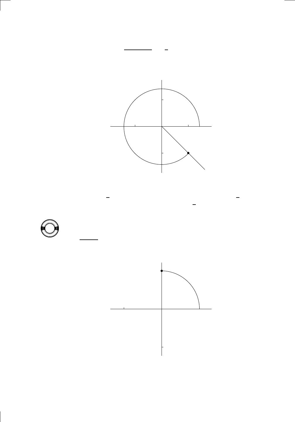
602 • Complex Numbers
1 + (−1)i; so we need to set x = 1 and y = −1 in the above formulas. Indeed,
if z = re
iθ
, then r =
p
1
2
+ (−1)
2
=
√
2, and tan(θ) = (−1)/1 = −1. Now,
you have to check the quadrant in order to get the correct value of θ. The
best way is to draw a diagram:
PSfrag replacements
(
a, b)
[
a, b]
(
a, b]
[
a, b)
(
a, ∞)
[
a, ∞)
(
−∞, b)
(
−∞, b]
(
−∞, ∞)
{
x : a < x < b}
{
x : a ≤ x ≤ b}
{
x : a < x ≤ b}
{
x : a ≤ x < b}
{
x : x ≥ a}
{
x : x > a}
{
x : x ≤ b}
{
x : x < b}
R
a
b
shadow
0
1
4
−
2
3
−
3
g(
x) = x
2
f(
x) = x
3
g(
x) = x
2
f(
x) = x
3
mirror (
y = x)
f
−
1
(x) =
3
√
x
y = h
(x)
y = h
−
1
(x)
y = (
x − 1)
2
−
1
x
Same height
−
x
Same length,
opposite signs
y = −
2x
−
2
1
y =
1
2
x − 1
2
−
1
y = 2
x
y = 10
x
y = 2
−
x
y = log
2
(
x)
4
3 units
mirror (
x-axis)
y = |
x|
y = |
log
2
(x)|
θ radians
θ units
30
◦
=
π
6
45
◦
=
π
4
60
◦
=
π
3
120
◦
=
2
π
3
135
◦
=
3
π
4
150
◦
=
5
π
6
90
◦
=
π
2
180
◦
= π
210
◦
=
7
π
6
225
◦
=
5
π
4
240
◦
=
4
π
3
270
◦
=
3
π
2
300
◦
=
5
π
3
315
◦
=
7
π
4
330
◦
=
11
π
6
0
◦
= 0 radians
θ
hyp
otenuse
opposite
adjacent
0 (
≡ 2π)
π
2
π
3
π
2
I
II
III
IV
θ
(
x, y)
x
y
r
7
π
6
reference angle
reference angle =
π
6
sin +
sin −
cos +
cos −
tan +
tan −
A
S
T
C
7
π
4
9
π
13
5
π
6
(this angle is
5
π
6
clockwise)
1
2
1
2
3
4
5
6
0
−
1
−
2
−
3
−
4
−
5
−
6
−
3π
−
5
π
2
−
2π
−
3
π
2
−
π
−
π
2
3
π
3
π
5
π
2
2
π
3
π
2
π
π
2
y = sin(
x)
1
0
−
1
−
3π
−
5
π
2
−
2π
−
3
π
2
−
π
−
π
2
3
π
5
π
2
2
π
2
π
3
π
2
π
π
2
y = sin(
x)
y = cos(
x)
−
π
2
π
2
y = tan(
x), −
π
2
< x <
π
2
0
−
π
2
π
2
y = tan(
x)
−
2π
−
3π
−
5
π
2
−
3
π
2
−
π
−
π
2
π
2
3
π
3
π
5
π
2
2
π
3
π
2
π
y = sec(
x)
y = csc(
x)
y = cot(
x)
y = f (
x)
−
1
1
2
y = g(
x)
3
y = h
(x)
4
5
−
2
f(
x) =
1
x
g(
x) =
1
x
2
etc.
0
1
π
1
2
π
1
3
π
1
4
π
1
5
π
1
6
π
1
7
π
g(
x) = sin
1
x
1
0
−
1
L
10
100
200
y =
π
2
y = −
π
2
y = tan
−
1
(x)
π
2
π
y =
sin(
x)
x
, x > 3
0
1
−
1
a
L
f(
x) = x sin (1/x)
(0 < x < 0
.3)
h
(x) = x
g(
x) = −x
a
L
lim
x
→a
+
f(x) = L
lim
x
→a
+
f(x) = ∞
lim
x
→a
+
f(x) = −∞
lim
x
→a
+
f(x) DNE
lim
x
→a
−
f(x) = L
lim
x
→a
−
f(x) = ∞
lim
x
→a
−
f(x) = −∞
lim
x
→a
−
f(x) DNE
M
}
lim
x
→a
−
f(x) = M
lim
x
→a
f(x) = L
lim
x
→a
f(x) DNE
lim
x
→∞
f(x) = L
lim
x
→∞
f(x) = ∞
lim
x
→∞
f(x) = −∞
lim
x
→∞
f(x) DNE
lim
x
→−∞
f(x) = L
lim
x
→−∞
f(x) = ∞
lim
x
→−∞
f(x) = −∞
lim
x
→−∞
f(x) DNE
lim
x →a
+
f(
x) = ∞
lim
x →a
+
f(
x) = −∞
lim
x →a
−
f(
x) = ∞
lim
x →a
−
f(
x) = −∞
lim
x →a
f(
x) = ∞
lim
x →a
f(
x) = −∞
lim
x →a
f(
x) DNE
y = f (
x)
a
y =
|
x|
x
1
−
1
y =
|
x + 2|
x + 2
1
−
1
−
2
1
2
3
4
a
a
b
y = x sin
1
x
y = x
y = −
x
a
b
c
d
C
a
b
c
d
−
1
0
1
2
3
time
y
t
u
(
t, f(t))
(
u, f(u))
time
y
t
u
y
x
(
x, f(x))
y = |
x|
(
z, f(z))
z
y = f (
x)
a
tangent at x = a
b
tangent at x = b
c
tangent at x = c
y = x
2
tangent
at x = −
1
u
v
uv
u + ∆
u
v + ∆
v
(
u + ∆u)(v + ∆v)
∆
u
∆
v
u
∆v
v∆
u
∆
u∆v
y = f (
x)
1
2
−
2
y = |
x
2
− 4|
y = x
2
− 4
y = −
2x + 5
y = g(
x)
1
2
3
4
5
6
7
8
9
0
−
1
−
2
−
3
−
4
−
5
−
6
y = f (
x)
3
−
3
3
−
3
0
−
1
2
easy
hard
flat
y = f
0
(
x)
3
−
3
0
−
1
2
1
−
1
y = sin(
x)
y = x
x
A
B
O
1
C
D
sin(
x)
tan(
x)
y =
sin(
x)
x
π
2
π
1
−
1
x = 0
a = 0
x > 0
a > 0
x < 0
a < 0
rest position
+
−
y = x
2
sin
1
x
N
A
B
H
a
b
c
O
H
A
B
C
D
h
r
R
θ
1000
2000
α
β
p
h
y = g(
x) = log
b
(x)
y = f(
x) = b
x
y = e
x
5
10
1
2
3
4
0
−
1
−
2
−
3
−
4
y = ln(
x)
y = cosh(
x)
y = sinh(
x)
y = tanh(
x)
y = sech(
x)
y = csch(
x)
y = coth(
x)
1
−
1
y = f (
x)
original function
inverse function
slope = 0 at (
x, y)
slope is infinite at (
y, x)
−
108
2
5
1
2
1
2
3
4
5
6
0
−
1
−
2
−
3
−
4
−
5
−
6
−
3π
−
5
π
2
−
2π
−
3
π
2
−
π
−
π
2
3
π
3
π
5
π
2
2
π
3
π
2
π
π
2
y = sin(
x)
1
0
−
1
−
3π
−
5
π
2
−
2π
−
3
π
2
−
π
−
π
2
3
π
5
π
2
2
π
2
π
3
π
2
π
π
2
y = sin(
x)
y = sin(
x), −
π
2
≤ x ≤
π
2
−
2
−
1
0
2
π
2
−
π
2
y = sin
−
1
(x)
y = cos(
x)
π
π
2
y = cos
−
1
(x)
−
π
2
1
x
α
β
y = tan(
x)
y = tan(
x)
1
y = tan
−
1
(x)
y = sec(
x)
y = sec
−
1
(x)
y = csc
−
1
(x)
y = cot
−
1
(x)
1
y = cosh
−
1
(x)
y = sinh
−
1
(x)
y = tanh
−
1
(x)
y = sech
−
1
(x)
y = csch
−
1
(x)
y = coth
−
1
(x)
(0
, 3)
(2
, −1)
(5
, 2)
(7
, 0)
(
−1, 44)
(0
, 1)
(1
, −12)
(2
, 305)
y = 1
2
(2
, 3)
y = f (
x)
y = g(
x)
a
b
c
a
b
c
s
c
0
c
1
(
a, f(a))
(
b, f(b))
1
2
1
2
3
4
5
6
0
−
1
−
2
−
3
−
4
−
5
−
6
−
3π
−
5
π
2
−
2π
−
3
π
2
−
π
−
π
2
3
π
3
π
5
π
2
2
π
3
π
2
π
π
2
y = sin(
x)
1
0
−
1
−
3π
−
5
π
2
−
2π
−
3
π
2
−
π
−
π
2
3
π
5
π
2
2
π
2
π
3
π
2
π
π
2
c
OR
Local maximum
Local minimum
Horizontal point of inflection
1
e
y = f
0
(
x)
y = f(
x) = x ln(x)
−
1
e
?
y = f(
x) = x
3
y = g(
x) = x
4
x
f(
x)
−
3
−
2
−
1
0
1
2
1
2
3
4
+
−
?
1
5
6
3
f
0
(
x)
2 −
1
2
√
6
2 +
1
2
√
6
f
00
(
x)
7
8
g
00
(
x)
f
00
(
x)
0
y =
(
x − 3)(x − 1)
2
x
3
(
x + 2)
y = x ln(
x)
1
e
−
1
e
5
−
108
2
α
β
2 −
1
2
√
6
2 +
1
2
√
6
y = x
2
(
x − 5)
3
−
e
−
1/2
√
3
e
−
1/2
√
3
−
e
−3/2
e
−
3/2
−
1
√
3
1
√
3
−
1
1
y = xe
−
3x
2
/2
y =
x
3
− 6
x
2
+ 13x − 8
x
28
2
600
500
400
300
200
100
0
−
100
−
200
−
300
−
400
−
500
−
600
0
10
−
10
5
−
5
20
−
20
15
−
15
0
4
5
6
x
P
0
(
x)
+
−
−
existing fence
new fence
enclosure
A
h
b
H
99
100
101
h
dA/dh
r
h
1
2
7
shallow
deep
LAND
SEA
N
y
z
s
t
3
11
9
L
(11)
√
11
y = L
(x)
y = f (
x)
11
y = L
(x)
y = f (
x)
F
P
a
a + ∆
x
f(
a + ∆x)
L
(a + ∆x)
f(
a)
error
df
∆
x
a
b
y = f (
x)
true zero
starting approximation
better approximation
v
t
3
5
50
40
60
4
20
30
25
t
1
t
2
t
3
t
4
t
n
−2
t
n
−1
t
0
= a
t
n
= b
v
1
v
2
v
3
v
4
v
n
−1
v
n
−
30
6
30
|
v|
a
b
p
q
c
v(
c)
v(
c
1
)
v(
c
2
)
v(
c
3
)
v(
c
4
)
v(
c
5
)
v(
c
6
)
t
1
t
2
t
3
t
4
t
5
c
1
c
2
c
3
c
4
c
5
c
6
t
0
=
a
t
6
=
b
t
16
=
b
t
10
=
b
a
b
x
y
y = f (
x)
1
2
y = x
5
0
−
2
y = 1
a
b
y = sin(
x)
π
−
π
0
−
1
−
2
0
2
4
y = x
2
0
1
2
3
4
2
n
4
n
6
n
2(
n−2)
n
2(
n−1)
n
2
n
n
= 2
width of each interval =
2
n
−
2
1
3
0
I
II
III
IV
4
y
dx
y = −
x
2
− 2x + 3
3
−
5
y = |−
x
2
− 2x + 3|
I
II
IIa
5
3
0
1
2
a
b
y = f (
x)
y = g(
x)
y = x
2
a
b
5
3
0
1
2
y =
√
x
2
√
2
2
2
dy
x
2
a
b
y = f (
x)
y = g(
x)
M
m
1
2
−
1
−
2
0
y = e
−
x
2
1
2
e
−
1/4
f
av
y = f
av
c
A
M
0
1
2
a
b
x
t
y = f(
t)
F (
x )
y = f(
t)
F (
x + h )
x + h
F (
x + h) − F (x)
f(
x)
1
2
y = sin(
x)
π
−
π
−
1
−
2
y =
1
x
y = x
2
1
2
1
−
1
y = ln
|x|
θ
a
x
a
x
p
a
2
− x
2
3
x
p
9 − x
2
p
x
2
+ a
2
x
a
p
x
2
+ 15
x
√
15
x
p
x
2
− a
2
a
x
p
x
2
− 4
2
x
−
p
x
2
− a
2
a
x
−
p
x
2
− 4
2
y = f (
x)
a
b
a + ε
ε
Z
b
a
+ε
f(x) dx
small
even smaller
y = g(
x)
infinite area
finite area
1
y =
1
x
y =
1
x
p
, p < 1 (typical)
y =
1
x
p
, p > 1 (typical)
a
1
a
2
a
3
a
4
a
5
a
6
a
7
a
8
1
2
3
4
5
6
7
8
n
a
n
x
y
y = f (
x)
(
a, f(a))
a
−
1
0
1
a
6
1
2
7
1
2
7
?
−
2
−
1
−
2
t = 0
t = π/
6
t = π/
4
t = π/
3
t = π/
2
3
0
t = −
2
t = −
3/2
t = ±
1
t = −
1/2
t = 0
t = 1
/2
t = 3
/2
t = 2
12
−
12
θ
r
P
θ
r
P
11
π
6
2
(
−1, −1)
wrong point
π
4
5
π
4
√
2
(0
, 1)
(0
, −3)
(
−2, 0)
π
2
3
π
2
π
r = 3 sin(θ)
3π
2
θ
2π
1
0
−1
−2
−3
0
3
2
−
3
2
0
r = 1 + 2 cos(θ)
2π
3
4π
3
0
π
0
pi
−
3
2
3π
2
1
2
3
0
−1
−2
−3
0 ≤ θ ≤
2π
3
0 ≤ θ ≤ π
0 ≤ θ ≤ 2π
r = 1 + cos(θ)
r = 1 +
3
4
cos(θ)
−
1
4
r = sin(2θ)
r = sin(3θ)
r =
1
π
θ
0 ≤ θ ≤ 4π
r =
2
1 + sin(θ)
−
π
4
≤ θ ≤
5π
4
0 ≤ θ ≤ 2π
0 ≤ θ ≤ π
−4
−5
4
5
f(θ)
f(θ + dθ)
θ
dθ
θ + dθ
approximating region
exact region
0 ≤ θ ≤ 2π
r = |1 + 2 cos(θ)|
2i
2 − 3i
−1
θ = 0
θ =
π
4
θ =
π
2
θ =
2π
3
θ = π
θ =
13π
12
θ =
3π
2
θ =
7π
4
1 = e
0
e
i
π
4
i = e
i
π
2
e
i
2π
3
−1 = e
iπ
e
i
13π
12
−i = e
i
3π
2
e
i
7π
4
i
−i
1
θ
1 − i
You can easily see that the point (1, −1) is in the fourth quadrant, so θ must
be equal to 7π/4. (Alternatively, you could write θ = −π/4.) So we just have
to package r =
√
2 and θ = 7π/4 together as re
iθ
to see that 1−i =
√
2e
i(7π/4)
.
(If you used θ = −π/4 instead, you’ll get 1 −i =
√
2e
−i(π/4)
. Remember, you
could add any integer multiple of 2π to θ and still be correct.)
Let’s revisit a couple of examples that might seem confusing. First, how
would you write 2i in polar form? Consider 2i as being 0 + 2i, so it is repre-
PSfrag replacements
(
a, b)
[
a, b]
(
a, b]
[
a, b)
(
a, ∞)
[
a, ∞)
(
−∞, b)
(
−∞, b]
(
−∞, ∞)
{
x : a < x < b}
{
x : a ≤ x ≤ b}
{
x : a < x ≤ b}
{
x : a ≤ x < b}
{
x : x ≥ a}
{
x : x > a}
{
x : x ≤ b}
{
x : x < b}
R
a
b
shadow
0
1
4
−
2
3
−
3
g(
x) = x
2
f(
x) = x
3
g(
x) = x
2
f(
x) = x
3
mirror (
y = x)
f
−
1
(x) =
3
√
x
y = h
(x)
y = h
−
1
(x)
y = (
x − 1)
2
−
1
x
Same height
−
x
Same length,
opposite signs
y = −
2x
−
2
1
y =
1
2
x − 1
2
−
1
y = 2
x
y = 10
x
y = 2
−
x
y = log
2
(
x)
4
3 units
mirror (
x-axis)
y = |
x|
y = |
log
2
(x)|
θ radians
θ units
30
◦
=
π
6
45
◦
=
π
4
60
◦
=
π
3
120
◦
=
2
π
3
135
◦
=
3
π
4
150
◦
=
5
π
6
90
◦
=
π
2
180
◦
= π
210
◦
=
7
π
6
225
◦
=
5
π
4
240
◦
=
4
π
3
270
◦
=
3
π
2
300
◦
=
5
π
3
315
◦
=
7
π
4
330
◦
=
11
π
6
0
◦
= 0 radians
θ
hyp
otenuse
opposite
adjacent
0 (
≡ 2π)
π
2
π
3
π
2
I
II
III
IV
θ
(
x, y)
x
y
r
7
π
6
reference angle
reference angle =
π
6
sin +
sin −
cos +
cos −
tan +
tan −
A
S
T
C
7
π
4
9
π
13
5
π
6
(this angle is
5
π
6
clockwise)
1
2
1
2
3
4
5
6
0
−
1
−
2
−
3
−
4
−
5
−
6
−
3π
−
5
π
2
−
2π
−
3
π
2
−
π
−
π
2
3
π
3
π
5
π
2
2
π
3
π
2
π
π
2
y = sin(
x)
1
0
−
1
−
3π
−
5
π
2
−
2π
−
3
π
2
−
π
−
π
2
3
π
5
π
2
2
π
2
π
3
π
2
π
π
2
y = sin(
x)
y = cos(
x)
−
π
2
π
2
y = tan(
x), −
π
2
< x <
π
2
0
−
π
2
π
2
y = tan(
x)
−
2π
−
3π
−
5
π
2
−
3
π
2
−
π
−
π
2
π
2
3
π
3
π
5
π
2
2
π
3
π
2
π
y = sec(
x)
y = csc(
x)
y = cot(
x)
y = f(
x)
−
1
1
2
y = g(
x)
3
y = h
(x)
4
5
−
2
f(
x) =
1
x
g(
x) =
1
x
2
etc.
0
1
π
1
2
π
1
3
π
1
4
π
1
5
π
1
6
π
1
7
π
g(
x) = sin
1
x
1
0
−
1
L
10
100
200
y =
π
2
y = −
π
2
y = tan
−
1
(x)
π
2
π
y =
sin(
x)
x
, x > 3
0
1
−
1
a
L
f(
x) = x sin (1/x)
(0 < x < 0
.3)
h
(x) = x
g(
x) = −x
a
L
lim
x
→a
+
f(x) = L
lim
x
→a
+
f(x) = ∞
lim
x
→a
+
f(x) = −∞
lim
x
→a
+
f(x) DNE
lim
x
→a
−
f(x) = L
lim
x
→a
−
f(x) = ∞
lim
x
→a
−
f(x) = −∞
lim
x
→a
−
f(x) DNE
M
}
lim
x
→a
−
f(x) = M
lim
x
→a
f(x) = L
lim
x
→a
f(x) DNE
lim
x
→∞
f(x) = L
lim
x
→∞
f(x) = ∞
lim
x
→∞
f(x) = −∞
lim
x
→∞
f(x) DNE
lim
x
→−∞
f(x) = L
lim
x
→−∞
f(x) = ∞
lim
x
→−∞
f(x) = −∞
lim
x
→−∞
f(x) DNE
lim
x →a
+
f(
x) = ∞
lim
x →a
+
f(
x) = −∞
lim
x →a
−
f(
x) = ∞
lim
x →a
−
f(
x) = −∞
lim
x →a
f(
x) = ∞
lim
x →a
f(
x) = −∞
lim
x →a
f(
x) DNE
y = f (
x)
a
y =
|
x|
x
1
−
1
y =
|
x + 2|
x + 2
1
−
1
−
2
1
2
3
4
a
a
b
y = x sin
1
x
y = x
y = −
x
a
b
c
d
C
a
b
c
d
−
1
0
1
2
3
time
y
t
u
(
t, f(t))
(
u, f(u))
time
y
t
u
y
x
(
x, f(x))
y = |
x|
(
z, f(z))
z
y = f(
x)
a
tangent at x = a
b
tangent at x = b
c
tangent at x = c
y = x
2
tangent
at x = −
1
u
v
uv
u + ∆
u
v + ∆
v
(
u + ∆u)(v + ∆v)
∆
u
∆
v
u
∆v
v∆
u
∆
u∆v
y = f(
x)
1
2
−
2
y = |
x
2
− 4|
y = x
2
− 4
y = −
2x + 5
y = g(
x)
1
2
3
4
5
6
7
8
9
0
−
1
−
2
−
3
−
4
−
5
−
6
y = f (
x)
3
−
3
3
−
3
0
−
1
2
easy
hard
flat
y = f
0
(
x)
3
−
3
0
−
1
2
1
−
1
y = sin(
x)
y = x
x
A
B
O
1
C
D
sin(
x)
tan(
x)
y =
sin(
x)
x
π
2
π
1
−
1
x = 0
a = 0
x > 0
a > 0
x < 0
a < 0
rest position
+
−
y = x
2
sin
1
x
N
A
B
H
a
b
c
O
H
A
B
C
D
h
r
R
θ
1000
2000
α
β
p
h
y = g(
x) = log
b
(x)
y = f(
x) = b
x
y = e
x
5
10
1
2
3
4
0
−
1
−
2
−
3
−
4
y = ln(
x)
y = cosh(
x)
y = sinh(
x)
y = tanh(
x)
y = sech(
x)
y = csch(
x)
y = coth(
x)
1
−
1
y = f(
x)
original function
inverse function
slope = 0 at (
x, y)
slope is infinite at (
y, x)
−
108
2
5
1
2
1
2
3
4
5
6
0
−
1
−
2
−
3
−
4
−
5
−
6
−
3π
−
5
π
2
−
2π
−
3
π
2
−
π
−
π
2
3
π
3
π
5
π
2
2
π
3
π
2
π
π
2
y = sin(
x)
1
0
−
1
−
3π
−
5
π
2
−
2π
−
3
π
2
−
π
−
π
2
3
π
5
π
2
2
π
2
π
3
π
2
π
π
2
y = sin(
x)
y = sin(
x), −
π
2
≤ x ≤
π
2
−
2
−
1
0
2
π
2
−
π
2
y = sin
−
1
(x)
y = cos(
x)
π
π
2
y = cos
−
1
(x)
−
π
2
1
x
α
β
y = tan(
x)
y = tan(
x)
1
y = tan
−
1
(x)
y = sec(
x)
y = sec
−
1
(x)
y = csc
−
1
(x)
y = cot
−
1
(x)
1
y = cosh
−
1
(x)
y = sinh
−
1
(x)
y = tanh
−
1
(x)
y = sech
−
1
(x)
y = csch
−
1
(x)
y = coth
−
1
(x)
(0
, 3)
(2
, −1)
(5
, 2)
(7
, 0)
(
−1, 44)
(0
, 1)
(1
, −12)
(2
, 305)
y = 1
2
(2
, 3)
y = f(
x)
y = g(
x)
a
b
c
a
b
c
s
c
0
c
1
(
a, f(a))
(
b, f(b))
1
2
1
2
3
4
5
6
0
−
1
−
2
−
3
−
4
−
5
−
6
−
3π
−
5
π
2
−
2π
−
3
π
2
−
π
−
π
2
3
π
3
π
5
π
2
2
π
3
π
2
π
π
2
y = sin(
x)
1
0
−
1
−
3π
−
5
π
2
−
2π
−
3
π
2
−
π
−
π
2
3
π
5
π
2
2
π
2
π
3
π
2
π
π
2
c
OR
Local maximum
Local minimum
Horizontal point of inflection
1
e
y = f
0
(
x)
y = f (
x) = x ln(x)
−
1
e
?
y = f(
x) = x
3
y = g(
x) = x
4
x
f(
x)
−
3
−
2
−
1
0
1
2
1
2
3
4
+
−
?
1
5
6
3
f
0
(
x)
2 −
1
2
√
6
2 +
1
2
√
6
f
00
(
x)
7
8
g
00
(
x)
f
00
(
x)
0
y =
(
x − 3)(x − 1)
2
x
3
(
x + 2)
y = x ln(
x)
1
e
−
1
e
5
−
108
2
α
β
2 −
1
2
√
6
2 +
1
2
√
6
y = x
2
(
x − 5)
3
−
e
−
1/2
√
3
e
−
1/2
√
3
−
e
−3/2
e
−
3/2
−
1
√
3
1
√
3
−
1
1
y = xe
−
3x
2
/2
y =
x
3
− 6
x
2
+ 13x − 8
x
28
2
600
500
400
300
200
100
0
−
100
−
200
−
300
−
400
−
500
−
600
0
10
−
10
5
−
5
20
−
20
15
−
15
0
4
5
6
x
P
0
(
x)
+
−
−
existing fence
new fence
enclosure
A
h
b
H
99
100
101
h
dA/dh
r
h
1
2
7
shallow
deep
LAND
SEA
N
y
z
s
t
3
11
9
L
(11)
√
11
y = L
(x)
y = f (
x)
11
y = L
(x)
y = f(
x)
F
P
a
a + ∆
x
f(
a + ∆x)
L
(a + ∆x)
f(
a)
error
df
∆
x
a
b
y = f(
x)
true zero
starting approximation
better approximation
v
t
3
5
50
40
60
4
20
30
25
t
1
t
2
t
3
t
4
t
n
−2
t
n
−1
t
0
= a
t
n
= b
v
1
v
2
v
3
v
4
v
n
−1
v
n
−
30
6
30
|
v|
a
b
p
q
c
v(
c)
v(
c
1
)
v(
c
2
)
v(
c
3
)
v(
c
4
)
v(
c
5
)
v(
c
6
)
t
1
t
2
t
3
t
4
t
5
c
1
c
2
c
3
c
4
c
5
c
6
t
0
=
a
t
6
=
b
t
16
=
b
t
10
=
b
a
b
x
y
y = f(
x)
1
2
y = x
5
0
−
2
y = 1
a
b
y = sin(
x)
π
−
π
0
−
1
−
2
0
2
4
y = x
2
0
1
2
3
4
2
n
4
n
6
n
2(
n−2)
n
2(
n−1)
n
2
n
n
= 2
width of each interval =
2
n
−
2
1
3
0
I
II
III
IV
4
y
dx
y = −
x
2
− 2x + 3
3
−
5
y = |−
x
2
− 2x + 3|
I
II
IIa
5
3
0
1
2
a
b
y = f (
x)
y = g(
x)
y = x
2
a
b
5
3
0
1
2
y =
√
x
2
√
2
2
2
dy
x
2
a
b
y = f(
x)
y = g(
x)
M
m
1
2
−
1
−
2
0
y = e
−
x
2
1
2
e
−
1/4
f
av
y = f
av
c
A
M
0
1
2
a
b
x
t
y = f (
t)
F (
x )
y = f (
t)
F (
x + h)
x + h
F (
x + h) − F (x)
f(
x)
1
2
y = sin(
x)
π
−
π
−
1
−
2
y =
1
x
y = x
2
1
2
1
−
1
y = ln
|x|
θ
a
x
a
x
p
a
2
− x
2
3
x
p
9 − x
2
p
x
2
+ a
2
x
a
p
x
2
+ 15
x
√
15
x
p
x
2
− a
2
a
x
p
x
2
− 4
2
x
−
p
x
2
− a
2
a
x
−
p
x
2
− 4
2
y = f(
x)
a
b
a + ε
ε
Z
b
a
+ε
f(x) dx
small
even smaller
y = g(
x)
infinite area
finite area
1
y =
1
x
y =
1
x
p
, p < 1 (typical)
y =
1
x
p
, p > 1 (typical)
a
1
a
2
a
3
a
4
a
5
a
6
a
7
a
8
1
2
3
4
5
6
7
8
n
a
n
x
y
y = f(
x)
(
a, f(a))
a
−
1
0
1
a
6
1
2
7
1
2
7
?
−
2
−
1
−
2
t = 0
t = π/
6
t = π/
4
t = π/
3
t = π/
2
3
0
t = −
2
t = −
3/2
t = ±
1
t = −
1/2
t = 0
t = 1
/2
t = 3
/2
t = 2
12
−
12
θ
r
P
θ
r
P
11
π
6
2
(−1, −1)
wrong point
π
4
5π
4
√
2
(0, 1)
(0, −3)
(−2, 0)
π
2
3π
2
π
r = 3 sin(θ)
3π
2
θ
2π
1
0
−1
−2
−3
0
3
2
−
3
2
0
r = 1 + 2 cos(θ)
2π
3
4π
3
0
π
0
pi
−
3
2
3π
2
1
2
3
0
−1
−2
−3
0 ≤ θ ≤
2π
3
0 ≤ θ ≤ π
0 ≤ θ ≤ 2π
r = 1 + cos(θ)
r = 1 +
3
4
cos(θ)
−
1
4
r = sin(2θ)
r = sin(3θ)
r =
1
π
θ
0 ≤ θ ≤ 4π
r =
2
1 + sin(θ)
−
π
4
≤ θ ≤
5π
4
0 ≤ θ ≤ 2π
0 ≤ θ ≤ π
−4
−5
4
5
f(θ)
f(θ + dθ)
θ
dθ
θ + dθ
approximating region
exact region
0 ≤ θ ≤ 2π
r = |1 + 2 cos(θ)|
2i
2 − 3i
−1
θ = 0
θ =
π
4
θ =
π
2
θ =
2π
3
θ = π
θ =
13π
12
θ =
3π
2
θ =
7π
4
1 = e
0
e
i
π
4
i = e
i
π
2
e
i
2π
3
−1 = e
iπ
e
i
13π
12
−i = e
i
3π
2
e
i
7π
4
i
−i
1
θ
1 − i
sented by the point (0, 2) in the complex plane. So, if 2i = re
iθ
, then we have
r =
√
0
2
+ 2
2
= 2, whereas tan(θ) = 2/0. Wait, that’s no good—you can’t
divide by 0. Let’s just draw a picture and see what θ should be:
PSfrag replacements
(
a, b)
[
a, b]
(
a, b]
[
a, b)
(
a, ∞)
[
a, ∞)
(
−∞, b)
(
−∞, b]
(
−∞, ∞)
{
x : a < x < b}
{
x : a ≤ x ≤ b}
{
x : a < x ≤ b}
{
x : a ≤ x < b}
{
x : x ≥ a}
{
x : x > a}
{
x : x ≤ b}
{
x : x < b}
R
a
b
shadow
0
1
4
−
2
3
−
3
g(
x) = x
2
f(
x) = x
3
g(
x) = x
2
f(
x) = x
3
mirror (
y = x)
f
−
1
(x) =
3
√
x
y = h
(x)
y = h
−
1
(x)
y = (
x − 1)
2
−
1
x
Same height
−
x
Same length,
opposite signs
y = −
2x
−
2
1
y =
1
2
x − 1
2
−
1
y = 2
x
y = 10
x
y = 2
−
x
y = log
2
(
x)
4
3 units
mirror (
x-axis)
y = |
x|
y = |
log
2
(x)|
θ radians
θ units
30
◦
=
π
6
45
◦
=
π
4
60
◦
=
π
3
120
◦
=
2
π
3
135
◦
=
3
π
4
150
◦
=
5
π
6
90
◦
=
π
2
180
◦
= π
210
◦
=
7
π
6
225
◦
=
5
π
4
240
◦
=
4
π
3
270
◦
=
3
π
2
300
◦
=
5
π
3
315
◦
=
7
π
4
330
◦
=
11
π
6
0
◦
= 0 radians
θ
hyp
otenuse
opposite
adjacent
0 (
≡ 2π)
π
2
π
3
π
2
I
II
III
IV
θ
(
x, y)
x
y
r
7
π
6
reference angle
reference angle =
π
6
sin +
sin −
cos +
cos −
tan +
tan −
A
S
T
C
7
π
4
9
π
13
5
π
6
(this angle is
5
π
6
clockwise)
1
2
1
2
3
4
5
6
0
−
1
−
2
−
3
−
4
−
5
−
6
−
3π
−
5
π
2
−
2π
−
3
π
2
−
π
−
π
2
3
π
3
π
5
π
2
2
π
3
π
2
π
π
2
y = sin(
x)
1
0
−
1
−
3π
−
5
π
2
−
2π
−
3
π
2
−
π
−
π
2
3
π
5
π
2
2
π
2
π
3
π
2
π
π
2
y = sin(
x)
y = cos(
x)
−
π
2
π
2
y = tan(
x), −
π
2
< x <
π
2
0
−
π
2
π
2
y = tan(
x)
−
2π
−
3π
−
5
π
2
−
3
π
2
−
π
−
π
2
π
2
3
π
3
π
5
π
2
2
π
3
π
2
π
y = sec(
x)
y = csc(
x)
y = cot(
x)
y = f (
x)
−
1
1
2
y = g(
x)
3
y = h
(x)
4
5
−
2
f(
x) =
1
x
g(
x) =
1
x
2
etc.
0
1
π
1
2
π
1
3
π
1
4
π
1
5
π
1
6
π
1
7
π
g(
x) = sin
1
x
1
0
−
1
L
10
100
200
y =
π
2
y = −
π
2
y = tan
−
1
(x)
π
2
π
y =
sin(
x)
x
, x > 3
0
1
−
1
a
L
f(
x) = x sin (1/x)
(0 < x < 0
.3)
h
(x) = x
g(
x) = −x
a
L
lim
x
→a
+
f(x) = L
lim
x
→a
+
f(x) = ∞
lim
x
→a
+
f(x) = −∞
lim
x
→a
+
f(x) DNE
lim
x
→a
−
f(x) = L
lim
x
→a
−
f(x) = ∞
lim
x
→a
−
f(x) = −∞
lim
x
→a
−
f(x) DNE
M
}
lim
x
→a
−
f(x) = M
lim
x
→a
f(x) = L
lim
x
→a
f(x) DNE
lim
x
→∞
f(x) = L
lim
x
→∞
f(x) = ∞
lim
x
→∞
f(x) = −∞
lim
x
→∞
f(x) DNE
lim
x
→−∞
f(x) = L
lim
x
→−∞
f(x) = ∞
lim
x
→−∞
f(x) = −∞
lim
x
→−∞
f(x) DNE
lim
x →a
+
f(
x) = ∞
lim
x →a
+
f(
x) = −∞
lim
x →a
−
f(
x) = ∞
lim
x →a
−
f(
x) = −∞
lim
x →a
f(
x) = ∞
lim
x →a
f(
x) = −∞
lim
x →a
f(
x) DNE
y = f (
x)
a
y =
|
x|
x
1
−
1
y =
|
x + 2|
x + 2
1
−
1
−
2
1
2
3
4
a
a
b
y = x sin
1
x
y = x
y = −
x
a
b
c
d
C
a
b
c
d
−
1
0
1
2
3
time
y
t
u
(
t, f(t))
(
u, f(u))
time
y
t
u
y
x
(
x, f(x))
y = |
x|
(
z, f(z))
z
y = f (
x)
a
tangent at x = a
b
tangent at x = b
c
tangent at x = c
y = x
2
tangent
at x = −
1
u
v
uv
u + ∆
u
v + ∆
v
(
u + ∆u)(v + ∆v)
∆
u
∆
v
u
∆v
v∆
u
∆
u∆v
y = f (
x)
1
2
−
2
y = |
x
2
− 4|
y = x
2
− 4
y = −
2x + 5
y = g(
x)
1
2
3
4
5
6
7
8
9
0
−
1
−
2
−
3
−
4
−
5
−
6
y = f (
x)
3
−
3
3
−
3
0
−
1
2
easy
hard
flat
y = f
0
(
x)
3
−
3
0
−
1
2
1
−
1
y = sin(
x)
y = x
x
A
B
O
1
C
D
sin(
x)
tan(
x)
y =
sin(
x)
x
π
2
π
1
−
1
x = 0
a = 0
x > 0
a > 0
x < 0
a < 0
rest position
+
−
y = x
2
sin
1
x
N
A
B
H
a
b
c
O
H
A
B
C
D
h
r
R
θ
1000
2000
α
β
p
h
y = g(
x) = log
b
(x)
y = f(
x) = b
x
y = e
x
5
10
1
2
3
4
0
−
1
−
2
−
3
−
4
y = ln(
x)
y = cosh(
x)
y = sinh(
x)
y = tanh(
x)
y = sech(
x)
y = csch(
x)
y = coth(
x)
1
−
1
y = f (
x)
original function
inverse function
slope = 0 at (
x, y)
slope is infinite at (
y, x)
−
108
2
5
1
2
1
2
3
4
5
6
0
−
1
−
2
−
3
−
4
−
5
−
6
−
3π
−
5
π
2
−
2π
−
3
π
2
−
π
−
π
2
3
π
3
π
5
π
2
2
π
3
π
2
π
π
2
y = sin(
x)
1
0
−
1
−
3π
−
5
π
2
−
2π
−
3
π
2
−
π
−
π
2
3
π
5
π
2
2
π
2
π
3
π
2
π
π
2
y = sin(
x)
y = sin(
x), −
π
2
≤ x ≤
π
2
−
2
−
1
0
2
π
2
−
π
2
y = sin
−
1
(x)
y = cos(
x)
π
π
2
y = cos
−
1
(x)
−
π
2
1
x
α
β
y = tan(
x)
y = tan(
x)
1
y = tan
−
1
(x)
y = sec(
x)
y = sec
−
1
(x)
y = csc
−
1
(x)
y = cot
−
1
(x)
1
y = cosh
−
1
(x)
y = sinh
−
1
(x)
y = tanh
−
1
(x)
y = sech
−
1
(x)
y = csch
−
1
(x)
y = coth
−
1
(x)
(0
, 3)
(2
, −1)
(5
, 2)
(7
, 0)
(
−1, 44)
(0
, 1)
(1
, −12)
(2
, 305)
y = 1
2
(2
, 3)
y = f (
x)
y = g(
x)
a
b
c
a
b
c
s
c
0
c
1
(
a, f(a))
(
b, f(b))
1
2
1
2
3
4
5
6
0
−
1
−
2
−
3
−
4
−
5
−
6
−
3π
−
5
π
2
−
2π
−
3
π
2
−
π
−
π
2
3
π
3
π
5
π
2
2
π
3
π
2
π
π
2
y = sin(
x)
1
0
−
1
−
3π
−
5
π
2
−
2π
−
3
π
2
−
π
−
π
2
3
π
5
π
2
2
π
2
π
3
π
2
π
π
2
c
OR
Local maximum
Local minimum
Horizontal point of inflection
1
e
y = f
0
(
x)
y = f(
x) = x ln(x)
−
1
e
?
y = f(
x) = x
3
y = g(
x) = x
4
x
f(
x)
−
3
−
2
−
1
0
1
2
1
2
3
4
+
−
?
1
5
6
3
f
0
(
x)
2 −
1
2
√
6
2 +
1
2
√
6
f
00
(
x)
7
8
g
00
(
x)
f
00
(
x)
0
y =
(
x − 3)(x − 1)
2
x
3
(
x + 2)
y = x ln(
x)
1
e
−
1
e
5
−
108
2
α
β
2 −
1
2
√
6
2 +
1
2
√
6
y = x
2
(
x − 5)
3
−
e
−
1/2
√
3
e
−
1/2
√
3
−
e
−3/2
e
−
3/2
−
1
√
3
1
√
3
−
1
1
y = xe
−
3x
2
/2
y =
x
3
− 6
x
2
+ 13x − 8
x
28
2
600
500
400
300
200
100
0
−
100
−
200
−
300
−
400
−
500
−
600
0
10
−
10
5
−
5
20
−
20
15
−
15
0
4
5
6
x
P
0
(
x)
+
−
−
existing fence
new fence
enclosure
A
h
b
H
99
100
101
h
dA/dh
r
h
1
2
7
shallow
deep
LAND
SEA
N
y
z
s
t
3
11
9
L
(11)
√
11
y = L
(x)
y = f (
x)
11
y = L
(x)
y = f (
x)
F
P
a
a + ∆
x
f(
a + ∆x)
L
(a + ∆x)
f(
a)
error
df
∆
x
a
b
y = f (
x)
true zero
starting approximation
better approximation
v
t
3
5
50
40
60
4
20
30
25
t
1
t
2
t
3
t
4
t
n
−2
t
n
−1
t
0
= a
t
n
= b
v
1
v
2
v
3
v
4
v
n
−1
v
n
−
30
6
30
|
v|
a
b
p
q
c
v(
c)
v(
c
1
)
v(
c
2
)
v(
c
3
)
v(
c
4
)
v(
c
5
)
v(
c
6
)
t
1
t
2
t
3
t
4
t
5
c
1
c
2
c
3
c
4
c
5
c
6
t
0
=
a
t
6
=
b
t
16
=
b
t
10
=
b
a
b
x
y
y = f (
x)
1
2
y = x
5
0
−
2
y = 1
a
b
y = sin(
x)
π
−
π
0
−
1
−
2
0
2
4
y = x
2
0
1
2
3
4
2
n
4
n
6
n
2(
n−2)
n
2(
n−1)
n
2
n
n
= 2
width of each interval =
2
n
−
2
1
3
0
I
II
III
IV
4
y
dx
y = −
x
2
− 2x + 3
3
−
5
y = |−
x
2
− 2x + 3|
I
II
IIa
5
3
0
1
2
a
b
y = f (
x)
y = g(
x)
y = x
2
a
b
5
3
0
1
2
y =
√
x
2
√
2
2
2
dy
x
2
a
b
y = f (
x)
y = g(
x)
M
m
1
2
−
1
−
2
0
y = e
−
x
2
1
2
e
−
1/4
f
av
y = f
av
c
A
M
0
1
2
a
b
x
t
y = f(
t)
F (
x )
y = f(
t)
F (
x + h )
x + h
F (
x + h) − F (x)
f(
x)
1
2
y = sin(
x)
π
−
π
−
1
−
2
y =
1
x
y = x
2
1
2
1
−
1
y = ln
|x|
θ
a
x
a
x
p
a
2
− x
2
3
x
p
9 − x
2
p
x
2
+ a
2
x
a
p
x
2
+ 15
x
√
15
x
p
x
2
− a
2
a
x
p
x
2
− 4
2
x
−
p
x
2
− a
2
a
x
−
p
x
2
− 4
2
y = f (
x)
a
b
a + ε
ε
Z
b
a
+ε
f(x) dx
small
even smaller
y = g(
x)
infinite area
finite area
1
y =
1
x
y =
1
x
p
, p < 1 (typical)
y =
1
x
p
, p > 1 (typical)
a
1
a
2
a
3
a
4
a
5
a
6
a
7
a
8
1
2
3
4
5
6
7
8
n
a
n
x
y
y = f (
x)
(
a, f(a))
a
−
1
0
1
a
6
1
2
7
1
2
7
?
−
2
−
1
−
2
t = 0
t = π/
6
t = π/
4
t = π/
3
t = π/
2
3
0
t = −
2
t = −
3/2
t = ±
1
t = −
1/2
t = 0
t = 1/2
t = 3/2
t = 2
12
−12
θ
r
P
θ
r
P
11π
6
2
(−1, −1)
wrong point
π
4
5π
4
√
2
(0, 1)
(0, −3)
(−2, 0)
π
2
3π
2
π
r = 3 sin(θ)
3π
2
θ
2π
1
0
−1
−2
−3
0
3
2
−
3
2
0
r = 1 + 2 cos(θ)
2π
3
4π
3
0
π
0
pi
−
3
2
3π
2
1
2
3
0
−1
−2
−3
0 ≤ θ ≤
2π
3
0 ≤ θ ≤ π
0 ≤ θ ≤ 2π
r = 1 + cos(θ)
r = 1 +
3
4
cos(θ)
−
1
4
r = sin(2θ)
r = sin(3θ)
r =
1
π
θ
0 ≤ θ ≤ 4π
r =
2
1 + sin(θ)
−
π
4
≤ θ ≤
5π
4
0 ≤ θ ≤ 2π
0 ≤ θ ≤ π
−4
−5
4
5
f(θ)
f(θ + dθ)
θ
dθ
θ + dθ
approximating region
exact region
0 ≤ θ ≤ 2π
r = |1 + 2 cos(θ)|
2i
2 − 3i
−1
θ = 0
θ =
π
4
θ =
π
2
θ =
2π
3
θ = π
θ =
13π
12
θ =
3π
2
θ =
7π
4
1 = e
0
e
i
π
4
i = e
i
π
2
e
i
2π
3
−1 = e
iπ
e
i
13π
12
−i = e
i
3π
2
e
i
7π
4
i
−i
1
θ
1 − i
2i
−2i
2
−2
OK, so θ = π/2 from the picture. This is actually consistent with our strange
value for tan(θ) above, since tan(π/2) is undefined. So, we have 2i = 2e
iπ/2
.
Of course, this is just twice our formula i = e
iπ/2
from the previous section.
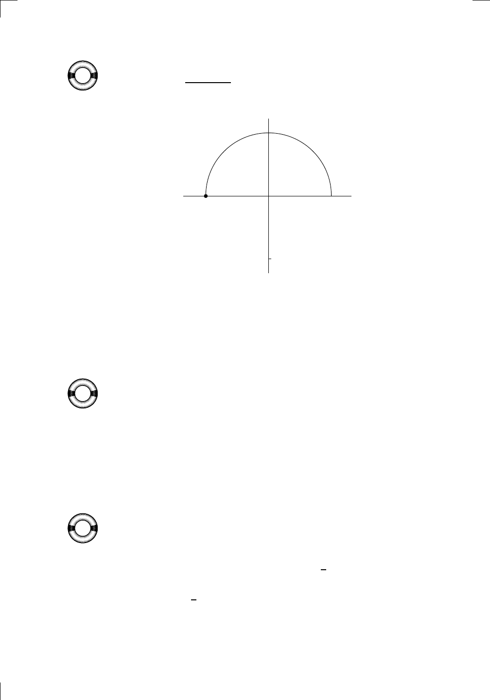
Section 28.3: Taking Large Powers of Complex Numbers • 603
How about changing −6 into polar form? Well, now we write −6 as −6+0i,
PSfrag
replacements
(
a, b)
[
a, b]
(
a, b]
[
a, b)
(
a, ∞)
[
a, ∞)
(
−∞, b)
(
−∞, b]
(
−∞, ∞)
{
x : a < x < b}
{
x : a ≤ x ≤ b}
{
x : a < x ≤ b}
{
x : a ≤ x < b}
{
x : x ≥ a}
{
x : x > a}
{
x : x ≤ b}
{
x : x < b}
R
a
b
shado
w
0
1
4
−
2
3
−
3
g(
x) = x
2
f(
x) = x
3
g(
x) = x
2
f(
x) = x
3
mirror
(y = x)
f
−
1
(x) =
3
√
x
y = h
(x)
y = h
−
1
(x)
y =
(x − 1)
2
−
1
x
Same
height
−
x
Same
length,
opp
osite signs
y = −
2x
−
2
1
y =
1
2
x − 1
2
−
1
y =
2
x
y =
10
x
y =
2
−x
y =
log
2
(x)
4
3
units
mirror
(x-axis)
y = |
x|
y = |
log
2
(x)|
θ radians
θ units
30
◦
=
π
6
45
◦
=
π
4
60
◦
=
π
3
120
◦
=
2
π
3
135
◦
=
3
π
4
150
◦
=
5
π
6
90
◦
=
π
2
180
◦
= π
210
◦
=
7
π
6
225
◦
=
5
π
4
240
◦
=
4
π
3
270
◦
=
3
π
2
300
◦
=
5
π
3
315
◦
=
7
π
4
330
◦
=
11
π
6
0
◦
=
0 radians
θ
hyp
otenuse
opp
osite
adjacen
t
0
(≡ 2π)
π
2
π
3
π
2
I
I
I
I
II
IV
θ
(
x, y)
x
y
r
7
π
6
reference
angle
reference
angle =
π
6
sin
+
sin −
cos
+
cos −
tan
+
tan −
A
S
T
C
7
π
4
9
π
13
5
π
6
(this
angle is
5π
6
clo
ckwise)
1
2
1
2
3
4
5
6
0
−
1
−
2
−
3
−
4
−
5
−
6
−
3π
−
5
π
2
−
2π
−
3
π
2
−
π
−
π
2
3
π
3
π
5
π
2
2
π
3
π
2
π
π
2
y =
sin(x)
1
0
−
1
−
3π
−
5
π
2
−
2π
−
3
π
2
−
π
−
π
2
3
π
5
π
2
2
π
2
π
3
π
2
π
π
2
y =
sin(x)
y =
cos(x)
−
π
2
π
2
y =
tan(x), −
π
2
<
x <
π
2
0
−
π
2
π
2
y =
tan(x)
−
2π
−
3π
−
5
π
2
−
3
π
2
−
π
−
π
2
π
2
3
π
3
π
5
π
2
2
π
3
π
2
π
y =
sec(x)
y =
csc(x)
y =
cot(x)
y = f(
x)
−
1
1
2
y = g(
x)
3
y = h
(x)
4
5
−
2
f(
x) =
1
x
g(
x) =
1
x
2
etc.
0
1
π
1
2
π
1
3
π
1
4
π
1
5
π
1
6
π
1
7
π
g(
x) = sin
1
x
1
0
−
1
L
10
100
200
y =
π
2
y = −
π
2
y =
tan
−1
(x)
π
2
π
y =
sin(
x)
x
,
x > 3
0
1
−
1
a
L
f(
x) = x sin (1/x)
(0 <
x < 0.3)
h
(x) = x
g(
x) = −x
a
L
lim
x
→a
+
f(x) = L
lim
x
→a
+
f(x) = ∞
lim
x
→a
+
f(x) = −∞
lim
x
→a
+
f(x) DNE
lim
x
→a
−
f(x) = L
lim
x
→a
−
f(x) = ∞
lim
x
→a
−
f(x) = −∞
lim
x
→a
−
f(x) DNE
M
}
lim
x
→a
−
f(x) = M
lim
x
→a
f(x) = L
lim
x
→a
f(x) DNE
lim
x
→∞
f(x) = L
lim
x
→∞
f(x) = ∞
lim
x
→∞
f(x) = −∞
lim
x
→∞
f(x) DNE
lim
x
→−∞
f(x) = L
lim
x
→−∞
f(x) = ∞
lim
x
→−∞
f(x) = −∞
lim
x
→−∞
f(x) DNE
lim
x →a
+
f(
x) = ∞
lim
x →a
+
f(
x) = −∞
lim
x →a
−
f(
x) = ∞
lim
x →a
−
f(
x) = −∞
lim
x →a
f(
x) = ∞
lim
x →a
f(
x) = −∞
lim
x →a
f(
x) DNE
y = f (
x)
a
y =
|
x|
x
1
−
1
y =
|
x + 2|
x +
2
1
−
1
−
2
1
2
3
4
a
a
b
y = x sin
1
x
y = x
y = −
x
a
b
c
d
C
a
b
c
d
−
1
0
1
2
3
time
y
t
u
(
t, f(t))
(
u, f(u))
time
y
t
u
y
x
(
x, f(x))
y = |
x|
(
z, f(z))
z
y = f(
x)
a
tangen
t at x = a
b
tangen
t at x = b
c
tangen
t at x = c
y = x
2
tangen
t
at x = −
1
u
v
uv
u +
∆u
v +
∆v
(
u + ∆u)(v + ∆v)
∆
u
∆
v
u
∆v
v∆
u
∆
u∆v
y = f(
x)
1
2
−
2
y = |
x
2
− 4|
y = x
2
− 4
y = −
2x + 5
y = g(
x)
1
2
3
4
5
6
7
8
9
0
−
1
−
2
−
3
−
4
−
5
−
6
y = f (
x)
3
−
3
3
−
3
0
−
1
2
easy
hard
flat
y = f
0
(
x)
3
−
3
0
−
1
2
1
−
1
y =
sin(x)
y = x
x
A
B
O
1
C
D
sin(
x)
tan(
x)
y =
sin(
x)
x
π
2
π
1
−
1
x =
0
a =
0
x
> 0
a
> 0
x
< 0
a
< 0
rest
position
+
−
y = x
2
sin
1
x
N
A
B
H
a
b
c
O
H
A
B
C
D
h
r
R
θ
1000
2000
α
β
p
h
y = g(
x) = log
b
(x)
y = f(
x) = b
x
y = e
x
5
10
1
2
3
4
0
−
1
−
2
−
3
−
4
y =
ln(x)
y =
cosh(x)
y =
sinh(x)
y =
tanh(x)
y =
sech(x)
y =
csch(x)
y =
coth(x)
1
−
1
y = f(
x)
original
function
in
verse function
slop
e = 0 at (x, y)
slop
e is infinite at (y, x)
−
108
2
5
1
2
1
2
3
4
5
6
0
−
1
−
2
−
3
−
4
−
5
−
6
−
3π
−
5
π
2
−
2π
−
3
π
2
−
π
−
π
2
3
π
3
π
5
π
2
2
π
3
π
2
π
π
2
y =
sin(x)
1
0
−
1
−
3π
−
5
π
2
−
2π
−
3
π
2
−
π
−
π
2
3
π
5
π
2
2
π
2
π
3
π
2
π
π
2
y =
sin(x)
y =
sin(x), −
π
2
≤ x ≤
π
2
−
2
−
1
0
2
π
2
−
π
2
y =
sin
−1
(x)
y =
cos(x)
π
π
2
y =
cos
−1
(x)
−
π
2
1
x
α
β
y =
tan(x)
y =
tan(x)
1
y =
tan
−1
(x)
y =
sec(x)
y =
sec
−1
(x)
y =
csc
−1
(x)
y =
cot
−1
(x)
1
y =
cosh
−1
(x)
y =
sinh
−1
(x)
y =
tanh
−1
(x)
y =
sech
−1
(x)
y =
csch
−1
(x)
y =
coth
−1
(x)
(0
, 3)
(2
, −1)
(5
, 2)
(7
, 0)
(
−1, 44)
(0
, 1)
(1
, −12)
(2
, 305)
y =
1
2
(2
, 3)
y = f(
x)
y = g(
x)
a
b
c
a
b
c
s
c
0
c
1
(
a, f(a))
(
b, f(b))
1
2
1
2
3
4
5
6
0
−
1
−
2
−
3
−
4
−
5
−
6
−
3π
−
5
π
2
−
2π
−
3
π
2
−
π
−
π
2
3
π
3
π
5
π
2
2
π
3
π
2
π
π
2
y =
sin(x)
1
0
−
1
−
3π
−
5
π
2
−
2π
−
3
π
2
−
π
−
π
2
3
π
5
π
2
2
π
2
π
3
π
2
π
π
2
c
OR
Lo
cal maximum
Lo
cal minimum
Horizon
tal point of inflection
1
e
y = f
0
(
x)
y = f (
x) = x ln(x)
−
1
e
?
y = f(
x) = x
3
y = g(
x) = x
4
x
f(
x)
−
3
−
2
−
1
0
1
2
1
2
3
4
+
−
?
1
5
6
3
f
0
(
x)
2 −
1
2
√
6
2
+
1
2
√
6
f
00
(
x)
7
8
g
00
(
x)
f
00
(
x)
0
y =
(
x − 3)(x − 1)
2
x
3
(
x + 2)
y = x ln
(x)
1
e
−
1
e
5
−
108
2
α
β
2 −
1
2
√
6
2
+
1
2
√
6
y = x
2
(
x − 5)
3
−
e
−
1/2
√
3
e
−
1/2
√
3
−
e
−3/2
e
−
3/2
−
1
√
3
1
√
3
−
1
1
y = xe
−
3x
2
/2
y =
x
3
− 6
x
2
+ 13x − 8
x
28
2
600
500
400
300
200
100
0
−
100
−
200
−
300
−
400
−
500
−
600
0
10
−
10
5
−
5
20
−
20
15
−
15
0
4
5
6
x
P
0
(
x)
+
−
−
existing
fence
new
fence
enclosure
A
h
b
H
99
100
101
h
dA/dh
r
h
1
2
7
shallo
w
deep
LAND
SEA
N
y
z
s
t
3
11
9
L
(11)
√
11
y = L
(x)
y = f (
x)
11
y = L
(x)
y = f(
x)
F
P
a
a +
∆x
f(
a + ∆x)
L
(a + ∆x)
f(
a)
error
d
f
∆
x
a
b
y = f(
x)
true
zero
starting
approximation
b
etter approximation
v
t
3
5
50
40
60
4
20
30
25
t
1
t
2
t
3
t
4
t
n
−2
t
n
−1
t
0
= a
t
n
= b
v
1
v
2
v
3
v
4
v
n
−1
v
n
−
30
6
30
|
v|
a
b
p
q
c
v(
c)
v(
c
1
)
v(
c
2
)
v(
c
3
)
v(
c
4
)
v(
c
5
)
v(
c
6
)
t
1
t
2
t
3
t
4
t
5
c
1
c
2
c
3
c
4
c
5
c
6
t
0
=
a
t
6
=
b
t
16
=
b
t
10
=
b
a
b
x
y
y = f(
x)
1
2
y = x
5
0
−
2
y =
1
a
b
y =
sin(x)
π
−
π
0
−
1
−
2
0
2
4
y = x
2
0
1
2
3
4
2
n
4
n
6
n
2(
n−2)
n
2(
n−1)
n
2
n
n
=
2
width
of each interval =
2
n
−
2
1
3
0
I
I
I
I
II
IV
4
y
dx
y = −
x
2
− 2x + 3
3
−
5
y = |−
x
2
− 2x + 3|
I
I
I
I
Ia
5
3
0
1
2
a
b
y = f (
x)
y = g(
x)
y = x
2
a
b
5
3
0
1
2
y =
√
x
2
√
2
2
2
dy
x
2
a
b
y = f(
x)
y = g(
x)
M
m
1
2
−
1
−
2
0
y = e
−
x
2
1
2
e
−
1/4
f
a
v
y = f
a
v
c
A
M
0
1
2
a
b
x
t
y = f (
t)
F (
x )
y = f (
t)
F (
x + h)
x + h
F (
x + h) − F (x)
f(
x)
1
2
y =
sin(x)
π
−
π
−
1
−
2
y =
1
x
y = x
2
1
2
1
−
1
y =
ln|x|
θ
a
x
a
x
p
a
2
− x
2
3
x
p
9 − x
2
p
x
2
+ a
2
x
a
p
x
2
+ 15
x
√
15
x
p
x
2
− a
2
a
x
p
x
2
− 4
2
x
−
p
x
2
− a
2
a
x
−
p
x
2
− 4
2
y = f(
x)
a
b
a + ε
ε
Z
b
a
+ε
f(x) dx
small
ev
en smaller
y = g(
x)
infinite
area
finite
area
1
y =
1
x
y =
1
x
p
, p
< 1 (typical)
y =
1
x
p
, p
> 1 (typical)
a
1
a
2
a
3
a
4
a
5
a
6
a
7
a
8
1
2
3
4
5
6
7
8
n
a
n
x
y
y = f(
x)
(
a, f(a))
a
−
1
0
1
a
6
1
2
7
1
2
7
?
−
2
−
1
−
2
t =
0
t = π
/6
t = π
/4
t = π
/3
t = π
/2
3
0
t = −
2
t = −
3/2
t = ±
1
t = −
1/2
t =
0
t =
1/2
t =
3/2
t =
2
12
−
12
θ
r
P
θ
r
P
11
π
6
2
(
−1, −1)
wrong
point
π
4
5
π
4
√
2
(0
, 1)
(0
, −3)
(
−2, 0)
π
2
3
π
2
π
r =
3 sin(θ)
3
π
2
θ
2
π
1
0
−
1
−
2
−
3
0
3
2
−
3
2
0
r =
1 + 2 cos(θ)
2
π
3
4
π
3
0
π
0
pi
−
3
2
3π
2
1
2
3
0
−1
−2
−3
0 ≤ θ ≤
2π
3
0 ≤ θ ≤ π
0 ≤ θ ≤ 2π
r = 1 + cos(θ)
r = 1 +
3
4
cos(θ)
−
1
4
r = sin(2θ)
r = sin(3θ)
r =
1
π
θ
0 ≤ θ ≤ 4π
r =
2
1 + sin(θ)
−
π
4
≤ θ ≤
5π
4
0 ≤ θ ≤ 2π
0 ≤ θ ≤ π
−4
−5
4
5
f(θ)
f(θ + dθ)
θ
dθ
θ + dθ
approximating region
exact region
0 ≤ θ ≤ 2π
r = |1 + 2 cos(θ)|
2i
2 − 3i
−1
θ = 0
θ =
π
4
θ =
π
2
θ =
2π
3
θ = π
θ =
13π
12
θ =
3π
2
θ =
7π
4
1 = e
0
e
i
π
4
i = e
i
π
2
e
i
2π
3
−1 = e
iπ
e
i
13π
12
−i = e
i
3π
2
e
i
7π
4
i
−i
1
θ
1 − i
2i
−2i
2
−2
and see that r =
p
(−6)
2
+ 0
2
= 6 and tan(θ) = 0/(−6) = 0. This means that
θ is an integer multiple of π, but to nail it down, let’s draw another picture:
PSfrag
replacements
(
a, b)
[
a, b]
(
a, b]
[
a, b)
(
a, ∞)
[
a, ∞)
(
−∞, b)
(
−∞, b]
(
−∞, ∞)
{
x : a < x < b}
{
x : a ≤ x ≤ b}
{
x : a < x ≤ b}
{
x : a ≤ x < b}
{
x : x ≥ a}
{
x : x > a}
{
x : x ≤ b}
{
x : x < b}
R
a
b
shado
w
0
1
4
−
2
3
−
3
g(
x) = x
2
f(
x) = x
3
g(
x) = x
2
f(
x) = x
3
mirror
(y = x)
f
−
1
(x) =
3
√
x
y = h
(x)
y = h
−
1
(x)
y =
(x − 1)
2
−
1
x
Same
height
−
x
Same
length,
opp
osite signs
y = −
2x
−
2
1
y =
1
2
x − 1
2
−
1
y =
2
x
y =
10
x
y =
2
−x
y =
log
2
(x)
4
3
units
mirror
(x-axis)
y = |
x|
y = |
log
2
(x)|
θ radians
θ units
30
◦
=
π
6
45
◦
=
π
4
60
◦
=
π
3
120
◦
=
2
π
3
135
◦
=
3
π
4
150
◦
=
5
π
6
90
◦
=
π
2
180
◦
= π
210
◦
=
7
π
6
225
◦
=
5
π
4
240
◦
=
4
π
3
270
◦
=
3
π
2
300
◦
=
5
π
3
315
◦
=
7
π
4
330
◦
=
11
π
6
0
◦
=
0 radians
θ
hyp
otenuse
opp
osite
adjacen
t
0
(≡ 2π)
π
2
π
3
π
2
I
I
I
I
II
IV
θ
(
x, y)
x
y
r
7
π
6
reference
angle
reference
angle =
π
6
sin
+
sin −
cos
+
cos −
tan
+
tan −
A
S
T
C
7
π
4
9
π
13
5
π
6
(this
angle is
5π
6
clo
ckwise)
1
2
1
2
3
4
5
6
0
−
1
−
2
−
3
−
4
−
5
−
6
−
3π
−
5
π
2
−
2π
−
3
π
2
−
π
−
π
2
3
π
3
π
5
π
2
2
π
3
π
2
π
π
2
y =
sin(x)
1
0
−
1
−
3π
−
5
π
2
−
2π
−
3
π
2
−
π
−
π
2
3
π
5
π
2
2
π
2
π
3
π
2
π
π
2
y =
sin(x)
y =
cos(x)
−
π
2
π
2
y =
tan(x), −
π
2
<
x <
π
2
0
−
π
2
π
2
y =
tan(x)
−
2π
−
3π
−
5
π
2
−
3
π
2
−
π
−
π
2
π
2
3
π
3
π
5
π
2
2
π
3
π
2
π
y =
sec(x)
y =
csc(x)
y =
cot(x)
y = f (
x)
−
1
1
2
y = g(
x)
3
y = h
(x)
4
5
−
2
f(
x) =
1
x
g(
x) =
1
x
2
etc.
0
1
π
1
2
π
1
3
π
1
4
π
1
5
π
1
6
π
1
7
π
g(
x) = sin
1
x
1
0
−
1
L
10
100
200
y =
π
2
y = −
π
2
y =
tan
−1
(x)
π
2
π
y =
sin(
x)
x
,
x > 3
0
1
−
1
a
L
f(
x) = x sin (1/x)
(0 <
x < 0.3)
h
(x) = x
g(
x) = −x
a
L
lim
x
→a
+
f(x) = L
lim
x
→a
+
f(x) = ∞
lim
x
→a
+
f(x) = −∞
lim
x
→a
+
f(x) DNE
lim
x
→a
−
f(x) = L
lim
x
→a
−
f(x) = ∞
lim
x
→a
−
f(x) = −∞
lim
x
→a
−
f(x) DNE
M
}
lim
x
→a
−
f(x) = M
lim
x
→a
f(x) = L
lim
x
→a
f(x) DNE
lim
x
→∞
f(x) = L
lim
x
→∞
f(x) = ∞
lim
x
→∞
f(x) = −∞
lim
x
→∞
f(x) DNE
lim
x
→−∞
f(x) = L
lim
x
→−∞
f(x) = ∞
lim
x
→−∞
f(x) = −∞
lim
x
→−∞
f(x) DNE
lim
x →a
+
f(
x) = ∞
lim
x →a
+
f(
x) = −∞
lim
x →a
−
f(
x) = ∞
lim
x →a
−
f(
x) = −∞
lim
x →a
f(
x) = ∞
lim
x →a
f(
x) = −∞
lim
x →a
f(
x) DNE
y = f (
x)
a
y =
|
x|
x
1
−
1
y =
|
x + 2|
x +
2
1
−
1
−
2
1
2
3
4
a
a
b
y = x sin
1
x
y = x
y = −
x
a
b
c
d
C
a
b
c
d
−
1
0
1
2
3
time
y
t
u
(
t, f(t))
(
u, f(u))
time
y
t
u
y
x
(
x, f(x))
y = |
x|
(
z, f(z))
z
y = f (
x)
a
tangen
t at x = a
b
tangen
t at x = b
c
tangen
t at x = c
y = x
2
tangen
t
at x = −
1
u
v
uv
u +
∆u
v +
∆v
(
u + ∆u)(v + ∆v)
∆
u
∆
v
u
∆v
v∆
u
∆
u∆v
y = f (
x)
1
2
−
2
y = |
x
2
− 4|
y = x
2
− 4
y = −
2x + 5
y = g(
x)
1
2
3
4
5
6
7
8
9
0
−
1
−
2
−
3
−
4
−
5
−
6
y = f (
x)
3
−
3
3
−
3
0
−
1
2
easy
hard
flat
y = f
0
(
x)
3
−
3
0
−
1
2
1
−
1
y =
sin(x)
y = x
x
A
B
O
1
C
D
sin(
x)
tan(
x)
y =
sin
(x)
x
π
2
π
1
−
1
x =
0
a =
0
x
> 0
a
> 0
x
< 0
a
< 0
rest
position
+
−
y = x
2
sin
1
x
N
A
B
H
a
b
c
O
H
A
B
C
D
h
r
R
θ
1000
2000
α
β
p
h
y = g(
x) = log
b
(x)
y = f(
x) = b
x
y = e
x
5
10
1
2
3
4
0
−
1
−
2
−
3
−
4
y =
ln(x)
y =
cosh(x)
y =
sinh(x)
y =
tanh(x)
y =
sech(x)
y =
csch(x)
y =
coth(x)
1
−
1
y = f (
x)
original
function
in
verse function
slop
e = 0 at (x, y)
slop
e is infinite at (y, x)
−
108
2
5
1
2
1
2
3
4
5
6
0
−
1
−
2
−
3
−
4
−
5
−
6
−
3π
−
5
π
2
−
2π
−
3
π
2
−
π
−
π
2
3
π
3
π
5
π
2
2
π
3
π
2
π
π
2
y =
sin(x)
1
0
−
1
−
3π
−
5
π
2
−
2π
−
3
π
2
−
π
−
π
2
3
π
5
π
2
2
π
2
π
3
π
2
π
π
2
y =
sin(x)
y =
sin(x), −
π
2
≤ x ≤
π
2
−
2
−
1
0
2
π
2
−
π
2
y =
sin
−1
(x)
y =
cos(x)
π
π
2
y =
cos
−1
(x)
−
π
2
1
x
α
β
y =
tan(x)
y =
tan(x)
1
y =
tan
−1
(x)
y =
sec(x)
y =
sec
−1
(x)
y =
csc
−1
(x)
y =
cot
−1
(x)
1
y =
cosh
−1
(x)
y =
sinh
−1
(x)
y =
tanh
−1
(x)
y =
sech
−1
(x)
y =
csch
−1
(x)
y =
coth
−1
(x)
(0
, 3)
(2
, −1)
(5
, 2)
(7
, 0)
(
−1, 44)
(0
, 1)
(1
, −12)
(2
, 305)
y =
1
2
(2
, 3)
y = f (
x)
y = g(
x)
a
b
c
a
b
c
s
c
0
c
1
(
a, f(a))
(
b, f(b))
1
2
1
2
3
4
5
6
0
−
1
−
2
−
3
−
4
−
5
−
6
−
3π
−
5
π
2
−
2π
−
3
π
2
−
π
−
π
2
3
π
3
π
5
π
2
2
π
3
π
2
π
π
2
y =
sin(x)
1
0
−
1
−
3π
−
5
π
2
−
2π
−
3
π
2
−
π
−
π
2
3
π
5
π
2
2
π
2
π
3
π
2
π
π
2
c
OR
Lo
cal maximum
Lo
cal minimum
Horizon
tal point of inflection
1
e
y = f
0
(
x)
y = f(
x) = x ln(x)
−
1
e
?
y = f(
x) = x
3
y = g(
x) = x
4
x
f(
x)
−
3
−
2
−
1
0
1
2
1
2
3
4
+
−
?
1
5
6
3
f
0
(
x)
2 −
1
2
√
6
2
+
1
2
√
6
f
00
(
x)
7
8
g
00
(
x)
f
00
(
x)
0
y =
(
x − 3)(x − 1)
2
x
3
(
x + 2)
y = x ln
(x)
1
e
−
1
e
5
−
108
2
α
β
2 −
1
2
√
6
2
+
1
2
√
6
y = x
2
(
x − 5)
3
−
e
−
1/2
√
3
e
−
1/2
√
3
−
e
−3/2
e
−
3/2
−
1
√
3
1
√
3
−
1
1
y = xe
−
3x
2
/2
y =
x
3
− 6
x
2
+ 13x − 8
x
28
2
600
500
400
300
200
100
0
−
100
−
200
−
300
−
400
−
500
−
600
0
10
−
10
5
−
5
20
−
20
15
−
15
0
4
5
6
x
P
0
(
x)
+
−
−
existing
fence
new
fence
enclosure
A
h
b
H
99
100
101
h
dA/dh
r
h
1
2
7
shallo
w
deep
LAND
SEA
N
y
z
s
t
3
11
9
L
(11)
√
11
y = L
(x)
y = f (
x)
11
y = L
(x)
y = f (
x)
F
P
a
a +
∆x
f(
a + ∆x)
L
(a + ∆x)
f(
a)
error
d
f
∆
x
a
b
y = f (
x)
true
zero
starting
approximation
b
etter approximation
v
t
3
5
50
40
60
4
20
30
25
t
1
t
2
t
3
t
4
t
n
−2
t
n
−1
t
0
= a
t
n
= b
v
1
v
2
v
3
v
4
v
n
−1
v
n
−
30
6
30
|
v|
a
b
p
q
c
v(
c)
v(
c
1
)
v(
c
2
)
v(
c
3
)
v(
c
4
)
v(
c
5
)
v(
c
6
)
t
1
t
2
t
3
t
4
t
5
c
1
c
2
c
3
c
4
c
5
c
6
t
0
=
a
t
6
=
b
t
16
=
b
t
10
=
b
a
b
x
y
y = f (
x)
1
2
y = x
5
0
−
2
y =
1
a
b
y =
sin(x)
π
−
π
0
−
1
−
2
0
2
4
y = x
2
0
1
2
3
4
2
n
4
n
6
n
2(
n−2)
n
2(
n−1)
n
2
n
n
=
2
width
of each interval =
2
n
−
2
1
3
0
I
I
I
I
II
IV
4
y
dx
y = −
x
2
− 2x + 3
3
−
5
y = |−
x
2
− 2x + 3|
I
I
I
I
Ia
5
3
0
1
2
a
b
y = f (
x)
y = g(
x)
y = x
2
a
b
5
3
0
1
2
y =
√
x
2
√
2
2
2
dy
x
2
a
b
y = f (
x)
y = g(
x)
M
m
1
2
−
1
−
2
0
y = e
−
x
2
1
2
e
−
1/4
f
a
v
y = f
a
v
c
A
M
0
1
2
a
b
x
t
y = f(
t)
F (
x )
y = f(
t)
F (
x + h )
x + h
F (
x + h) − F (x)
f(
x)
1
2
y =
sin(x)
π
−
π
−
1
−
2
y =
1
x
y = x
2
1
2
1
−
1
y =
ln|x|
θ
a
x
a
x
p
a
2
− x
2
3
x
p
9 − x
2
p
x
2
+ a
2
x
a
p
x
2
+ 15
x
√
15
x
p
x
2
− a
2
a
x
p
x
2
− 4
2
x
−
p
x
2
− a
2
a
x
−
p
x
2
− 4
2
y = f (
x)
a
b
a + ε
ε
Z
b
a
+ε
f(x) dx
small
ev
en smaller
y = g(
x)
infinite
area
finite
area
1
y =
1
x
y =
1
x
p
, p
< 1 (typical)
y =
1
x
p
, p
> 1 (typical)
a
1
a
2
a
3
a
4
a
5
a
6
a
7
a
8
1
2
3
4
5
6
7
8
n
a
n
x
y
y = f (
x)
(
a, f(a))
a
−
1
0
1
a
6
1
2
7
1
2
7
?
−
2
−
1
−
2
t =
0
t = π
/6
t = π
/4
t = π
/3
t = π
/2
3
0
t = −
2
t = −
3/2
t = ±
1
t = −
1/2
t =
0
t =
1/2
t =
3/2
t =
2
12
−
12
θ
r
P
θ
r
P
11
π
6
2
(
−1, −1)
wrong
point
π
4
5
π
4
√
2
(0
, 1)
(0
, −3)
(
−2, 0)
π
2
3
π
2
π
r =
3 sin(θ)
3
π
2
θ
2
π
1
0
−
1
−
2
−3
0
3
2
−
3
2
0
r = 1 + 2 cos(θ)
2π
3
4π
3
0
π
0
pi
−
3
2
3π
2
1
2
3
0
−1
−2
−3
0 ≤ θ ≤
2π
3
0 ≤ θ ≤ π
0 ≤ θ ≤ 2π
r = 1 + cos(θ)
r = 1 +
3
4
cos(θ)
−
1
4
r = sin(2θ)
r = sin(3θ)
r =
1
π
θ
0 ≤ θ ≤ 4π
r =
2
1 + sin(θ)
−
π
4
≤ θ ≤
5π
4
0 ≤ θ ≤ 2π
0 ≤ θ ≤ π
−4
−5
4
5
f(θ)
f(θ + dθ)
θ
dθ
θ + dθ
approximating region
exact region
0 ≤ θ ≤ 2π
r = |1 + 2 cos(θ)|
2i
2 − 3i
−1
θ = 0
θ =
π
4
θ =
π
2
θ =
2π
3
θ = π
θ =
13π
12
θ =
3π
2
θ =
7π
4
1 = e
0
e
i
π
4
i = e
i
π
2
e
i
2π
3
−1 = e
iπ
e
i
13π
12
−i = e
i
3π
2
e
i
7π
4
i
−i
1
θ
1 − i
2i
−2i
2
−2
6i
−6i
6
−6
Now we see that θ = π (or if you prefer, −π, or even 3π, or any odd multiple
of π). So, we have −6 = 6e
iπ
. Incidentally, if we divide by 6, we get the
amazing formula e
iπ
= −1, which we discussed in the previous section.
28.3 Taking Large Powers of Complex Numbers
Why on earth would you want to use the polar form? One reason is that it’s
really easy to multiply and take powers in polar form. Imagine you wanted to
multiply 3e
iπ/4
by 2e
−i(3π/8)
. This is pretty simple—you just use the normal
PSfrag
replacements
(
a, b)
[
a, b]
(
a, b]
[
a, b)
(
a, ∞)
[
a, ∞)
(
−∞, b)
(
−∞, b]
(
−∞, ∞)
{
x : a < x < b}
{
x : a ≤ x ≤ b}
{
x : a < x ≤ b}
{
x : a ≤ x < b}
{
x : x ≥ a}
{
x : x > a}
{
x : x ≤ b}
{
x : x < b}
R
a
b
shado
w
0
1
4
−
2
3
−
3
g(
x) = x
2
f(
x) = x
3
g(
x) = x
2
f(
x) = x
3
mirror
(y = x)
f
−
1
(x) =
3
√
x
y = h
(x)
y = h
−
1
(x)
y =
(x − 1)
2
−
1
x
Same
height
−
x
Same
length,
opp
osite signs
y = −
2x
−
2
1
y =
1
2
x − 1
2
−
1
y =
2
x
y =
10
x
y =
2
−x
y =
log
2
(x)
4
3
units
mirror
(x-axis)
y = |
x|
y = |
log
2
(x)|
θ radians
θ units
30
◦
=
π
6
45
◦
=
π
4
60
◦
=
π
3
120
◦
=
2
π
3
135
◦
=
3
π
4
150
◦
=
5
π
6
90
◦
=
π
2
180
◦
= π
210
◦
=
7
π
6
225
◦
=
5
π
4
240
◦
=
4
π
3
270
◦
=
3
π
2
300
◦
=
5
π
3
315
◦
=
7
π
4
330
◦
=
11
π
6
0
◦
=
0 radians
θ
hyp
otenuse
opp
osite
adjacen
t
0
(≡ 2π)
π
2
π
3
π
2
I
I
I
I
II
IV
θ
(
x, y)
x
y
r
7
π
6
reference
angle
reference
angle =
π
6
sin
+
sin −
cos
+
cos −
tan
+
tan −
A
S
T
C
7
π
4
9
π
13
5
π
6
(this
angle is
5π
6
clo
ckwise)
1
2
1
2
3
4
5
6
0
−
1
−
2
−
3
−
4
−
5
−
6
−
3π
−
5
π
2
−
2π
−
3
π
2
−
π
−
π
2
3
π
3
π
5
π
2
2
π
3
π
2
π
π
2
y =
sin(x)
1
0
−
1
−
3π
−
5
π
2
−
2π
−
3
π
2
−
π
−
π
2
3
π
5
π
2
2
π
2
π
3
π
2
π
π
2
y =
sin(x)
y =
cos(x)
−
π
2
π
2
y =
tan(x), −
π
2
<
x <
π
2
0
−
π
2
π
2
y =
tan(x)
−
2π
−
3π
−
5
π
2
−
3
π
2
−
π
−
π
2
π
2
3
π
3
π
5
π
2
2
π
3
π
2
π
y =
sec(x)
y =
csc(x)
y =
cot(x)
y = f(
x)
−
1
1
2
y = g(
x)
3
y = h
(x)
4
5
−
2
f(
x) =
1
x
g(
x) =
1
x
2
etc.
0
1
π
1
2
π
1
3
π
1
4
π
1
5
π
1
6
π
1
7
π
g(
x) = sin
1
x
1
0
−
1
L
10
100
200
y =
π
2
y = −
π
2
y =
tan
−1
(x)
π
2
π
y =
sin(
x)
x
,
x > 3
0
1
−
1
a
L
f(
x) = x sin (1/x)
(0 <
x < 0.3)
h
(x) = x
g(
x) = −x
a
L
lim
x
→a
+
f(x) = L
lim
x
→a
+
f(x) = ∞
lim
x
→a
+
f(x) = −∞
lim
x
→a
+
f(x) DNE
lim
x
→a
−
f(x) = L
lim
x
→a
−
f(x) = ∞
lim
x
→a
−
f(x) = −∞
lim
x
→a
−
f(x) DNE
M
}
lim
x
→a
−
f(x) = M
lim
x
→a
f(x) = L
lim
x
→a
f(x) DNE
lim
x
→∞
f(x) = L
lim
x
→∞
f(x) = ∞
lim
x
→∞
f(x) = −∞
lim
x
→∞
f(x) DNE
lim
x
→−∞
f(x) = L
lim
x
→−∞
f(x) = ∞
lim
x
→−∞
f(x) = −∞
lim
x
→−∞
f(x) DNE
lim
x →a
+
f(
x) = ∞
lim
x →a
+
f(
x) = −∞
lim
x →a
−
f(
x) = ∞
lim
x →a
−
f(
x) = −∞
lim
x →a
f(
x) = ∞
lim
x →a
f(
x) = −∞
lim
x →a
f(
x) DNE
y = f (
x)
a
y =
|
x|
x
1
−
1
y =
|
x + 2|
x +
2
1
−
1
−
2
1
2
3
4
a
a
b
y = x sin
1
x
y = x
y = −
x
a
b
c
d
C
a
b
c
d
−
1
0
1
2
3
time
y
t
u
(
t, f(t))
(
u, f(u))
time
y
t
u
y
x
(
x, f(x))
y = |
x|
(
z, f(z))
z
y = f(
x)
a
tangen
t at x = a
b
tangen
t at x = b
c
tangen
t at x = c
y = x
2
tangen
t
at x = −
1
u
v
uv
u +
∆u
v +
∆v
(
u + ∆u)(v + ∆v)
∆
u
∆
v
u
∆v
v∆
u
∆
u∆v
y = f(
x)
1
2
−
2
y = |
x
2
− 4|
y = x
2
− 4
y = −
2x + 5
y = g(
x)
1
2
3
4
5
6
7
8
9
0
−
1
−
2
−
3
−
4
−
5
−
6
y = f (
x)
3
−
3
3
−
3
0
−
1
2
easy
hard
flat
y = f
0
(
x)
3
−
3
0
−
1
2
1
−
1
y =
sin(x)
y = x
x
A
B
O
1
C
D
sin(
x)
tan(
x)
y =
sin(
x)
x
π
2
π
1
−
1
x =
0
a =
0
x
> 0
a
> 0
x
< 0
a
< 0
rest
position
+
−
y = x
2
sin
1
x
N
A
B
H
a
b
c
O
H
A
B
C
D
h
r
R
θ
1000
2000
α
β
p
h
y = g(
x) = log
b
(x)
y = f(
x) = b
x
y = e
x
5
10
1
2
3
4
0
−
1
−
2
−
3
−
4
y =
ln(x)
y =
cosh(x)
y =
sinh(x)
y =
tanh(x)
y =
sech(x)
y =
csch(x)
y =
coth(x)
1
−
1
y = f(
x)
original
function
in
verse function
slop
e = 0 at (x, y)
slop
e is infinite at (y, x)
−
108
2
5
1
2
1
2
3
4
5
6
0
−
1
−
2
−
3
−
4
−
5
−
6
−
3π
−
5
π
2
−
2π
−
3
π
2
−
π
−
π
2
3
π
3
π
5
π
2
2
π
3
π
2
π
π
2
y =
sin(x)
1
0
−
1
−
3π
−
5
π
2
−
2π
−
3
π
2
−
π
−
π
2
3
π
5
π
2
2
π
2
π
3
π
2
π
π
2
y =
sin(x)
y =
sin(x), −
π
2
≤ x ≤
π
2
−
2
−
1
0
2
π
2
−
π
2
y =
sin
−1
(x)
y =
cos(x)
π
π
2
y =
cos
−1
(x)
−
π
2
1
x
α
β
y =
tan(x)
y =
tan(x)
1
y =
tan
−1
(x)
y =
sec(x)
y =
sec
−1
(x)
y =
csc
−1
(x)
y =
cot
−1
(x)
1
y =
cosh
−1
(x)
y =
sinh
−1
(x)
y =
tanh
−1
(x)
y =
sech
−1
(x)
y =
csch
−1
(x)
y =
coth
−1
(x)
(0
, 3)
(2
, −1)
(5
, 2)
(7
, 0)
(
−1, 44)
(0
, 1)
(1
, −12)
(2
, 305)
y =
1
2
(2
, 3)
y = f(
x)
y = g(
x)
a
b
c
a
b
c
s
c
0
c
1
(
a, f(a))
(
b, f(b))
1
2
1
2
3
4
5
6
0
−
1
−
2
−
3
−
4
−
5
−
6
−
3π
−
5
π
2
−
2π
−
3
π
2
−
π
−
π
2
3
π
3
π
5
π
2
2
π
3
π
2
π
π
2
y =
sin(x)
1
0
−
1
−
3π
−
5
π
2
−
2π
−
3
π
2
−
π
−
π
2
3
π
5
π
2
2
π
2
π
3
π
2
π
π
2
c
OR
Lo
cal maximum
Lo
cal minimum
Horizon
tal point of inflection
1
e
y = f
0
(
x)
y = f (
x) = x ln(x)
−
1
e
?
y = f(
x) = x
3
y = g(
x) = x
4
x
f(
x)
−
3
−
2
−
1
0
1
2
1
2
3
4
+
−
?
1
5
6
3
f
0
(
x)
2 −
1
2
√
6
2
+
1
2
√
6
f
00
(
x)
7
8
g
00
(
x)
f
00
(
x)
0
y =
(
x − 3)(x − 1)
2
x
3
(
x + 2)
y = x ln
(x)
1
e
−
1
e
5
−
108
2
α
β
2 −
1
2
√
6
2
+
1
2
√
6
y = x
2
(
x − 5)
3
−
e
−
1/2
√
3
e
−
1/2
√
3
−
e
−3/2
e
−
3/2
−
1
√
3
1
√
3
−
1
1
y = xe
−
3x
2
/2
y =
x
3
− 6
x
2
+ 13x − 8
x
28
2
600
500
400
300
200
100
0
−
100
−
200
−
300
−
400
−
500
−
600
0
10
−
10
5
−
5
20
−
20
15
−
15
0
4
5
6
x
P
0
(
x)
+
−
−
existing
fence
new
fence
enclosure
A
h
b
H
99
100
101
h
dA/dh
r
h
1
2
7
shallo
w
deep
LAND
SEA
N
y
z
s
t
3
11
9
L
(11)
√
11
y = L
(x)
y = f (
x)
11
y = L
(x)
y = f(
x)
F
P
a
a +
∆x
f(
a + ∆x)
L
(a + ∆x)
f(
a)
error
d
f
∆
x
a
b
y = f(
x)
true
zero
starting
approximation
b
etter approximation
v
t
3
5
50
40
60
4
20
30
25
t
1
t
2
t
3
t
4
t
n
−2
t
n
−1
t
0
= a
t
n
= b
v
1
v
2
v
3
v
4
v
n
−1
v
n
−
30
6
30
|
v|
a
b
p
q
c
v(
c)
v(
c
1
)
v(
c
2
)
v(
c
3
)
v(
c
4
)
v(
c
5
)
v(
c
6
)
t
1
t
2
t
3
t
4
t
5
c
1
c
2
c
3
c
4
c
5
c
6
t
0
=
a
t
6
=
b
t
16
=
b
t
10
=
b
a
b
x
y
y = f(
x)
1
2
y = x
5
0
−
2
y =
1
a
b
y =
sin(x)
π
−
π
0
−
1
−
2
0
2
4
y = x
2
0
1
2
3
4
2
n
4
n
6
n
2(
n−2)
n
2(
n−1)
n
2
n
n
=
2
width
of each interval =
2
n
−
2
1
3
0
I
I
I
I
II
IV
4
y
dx
y = −
x
2
− 2x + 3
3
−
5
y = |−
x
2
− 2x + 3|
I
I
I
I
Ia
5
3
0
1
2
a
b
y = f (
x)
y = g(
x)
y = x
2
a
b
5
3
0
1
2
y =
√
x
2
√
2
2
2
dy
x
2
a
b
y = f(
x)
y = g(
x)
M
m
1
2
−
1
−
2
0
y = e
−
x
2
1
2
e
−
1/4
f
a
v
y = f
a
v
c
A
M
0
1
2
a
b
x
t
y = f (
t)
F (
x )
y = f (
t)
F (
x + h)
x + h
F (
x + h) − F (x)
f(
x)
1
2
y =
sin(x)
π
−
π
−
1
−
2
y =
1
x
y = x
2
1
2
1
−
1
y =
ln|x|
θ
a
x
a
x
p
a
2
− x
2
3
x
p
9 − x
2
p
x
2
+ a
2
x
a
p
x
2
+ 15
x
√
15
x
p
x
2
− a
2
a
x
p
x
2
− 4
2
x
−
p
x
2
− a
2
a
x
−
p
x
2
− 4
2
y = f(
x)
a
b
a + ε
ε
Z
b
a
+ε
f(x) dx
small
ev
en smaller
y = g(
x)
infinite
area
finite
area
1
y =
1
x
y =
1
x
p
, p
< 1 (typical)
y =
1
x
p
, p
> 1 (typical)
a
1
a
2
a
3
a
4
a
5
a
6
a
7
a
8
1
2
3
4
5
6
7
8
n
a
n
x
y
y = f(
x)
(
a, f(a))
a
−
1
0
1
a
6
1
2
7
1
2
7
?
−
2
−
1
−
2
t =
0
t = π
/6
t = π
/4
t = π
/3
t = π
/2
3
0
t = −
2
t = −
3/2
t = ±
1
t = −
1/2
t =
0
t =
1/2
t =
3/2
t =
2
12
−
12
θ
r
P
θ
r
P
11
π
6
2
(
−1, −1)
wrong
point
π
4
5
π
4
√
2
(0
, 1)
(0
, −3)
(−2, 0)
π
2
3π
2
π
r = 3 sin(θ)
3π
2
θ
2π
1
0
−1
−2
−3
0
3
2
−
3
2
0
r = 1 + 2 cos(θ)
2π
3
4π
3
0
π
0
pi
−
3
2
3π
2
1
2
3
0
−1
−2
−3
0 ≤ θ ≤
2π
3
0 ≤ θ ≤ π
0 ≤ θ ≤ 2π
r = 1 + cos(θ)
r = 1 +
3
4
cos(θ)
−
1
4
r = sin(2θ)
r = sin(3θ)
r =
1
π
θ
0 ≤ θ ≤ 4π
r =
2
1 + sin(θ)
−
π
4
≤ θ ≤
5π
4
0 ≤ θ ≤ 2π
0 ≤ θ ≤ π
−4
−5
4
5
f(θ)
f(θ + dθ)
θ
dθ
θ + dθ
approximating region
exact region
0 ≤ θ ≤ 2π
r = |1 + 2 cos(θ)|
2i
2 − 3i
−1
θ = 0
θ =
π
4
θ =
π
2
θ =
2π
3
θ = π
θ =
13π
12
θ =
3π
2
θ =
7π
4
1 = e
0
e
i
π
4
i = e
i
π
2
e
i
2π
3
−1 = e
iπ
e
i
13π
12
−i = e
i
3π
2
e
i
7π
4
i
−i
1
θ
1 − i
2i
−2i
2
−2
6i
−6i
6
−6
exponential rules (see Section 9.1.1 in Chapter 9) to write
(3e
iπ/4
)(2e
−i(3π/8)
) = 6e
i(π/4−3π/8)
= 6e
−iπ/8
.
Even better, imagine you want to raise 3e
iπ/4
to the 200th power. This is just
(3e
iπ/4
)
200
= 3
200
e
(iπ/4)×200
= 3
200
e
i(50π)
.
In fact, by Euler’s identity, e
i(50π)
= cos(50π) + i sin(50π). Since 50π is an
integer multiple of 2π, we have cos(50π) = 1 and sin(50π) = 0, so we have
proved that (3e
iπ/4
)
200
= 3
200
.
A lot of the time, you might want the final answer in Cartesian form.
For example, suppose we’d like to compute (1 − i)
99
and give the answer in
PSfrag
replacements
(
a, b)
[
a, b]
(
a, b]
[
a, b)
(
a, ∞)
[
a, ∞)
(
−∞, b)
(
−∞, b]
(
−∞, ∞)
{
x : a < x < b}
{
x : a ≤ x ≤ b}
{
x : a < x ≤ b}
{
x : a ≤ x < b}
{
x : x ≥ a}
{
x : x > a}
{
x : x ≤ b}
{
x : x < b}
R
a
b
shado
w
0
1
4
−
2
3
−
3
g(
x) = x
2
f(
x) = x
3
g(
x) = x
2
f(
x) = x
3
mirror
(y = x)
f
−
1
(x) =
3
√
x
y = h
(x)
y = h
−
1
(x)
y =
(x − 1)
2
−
1
x
Same
height
−
x
Same
length,
opp
osite signs
y = −
2x
−
2
1
y =
1
2
x − 1
2
−
1
y =
2
x
y =
10
x
y =
2
−x
y =
log
2
(x)
4
3
units
mirror
(x-axis)
y = |
x|
y = |
log
2
(x)|
θ radians
θ units
30
◦
=
π
6
45
◦
=
π
4
60
◦
=
π
3
120
◦
=
2
π
3
135
◦
=
3
π
4
150
◦
=
5
π
6
90
◦
=
π
2
180
◦
= π
210
◦
=
7
π
6
225
◦
=
5
π
4
240
◦
=
4
π
3
270
◦
=
3
π
2
300
◦
=
5
π
3
315
◦
=
7
π
4
330
◦
=
11
π
6
0
◦
=
0 radians
θ
hyp
otenuse
opp
osite
adjacen
t
0
(≡ 2π)
π
2
π
3
π
2
I
I
I
I
II
IV
θ
(
x, y)
x
y
r
7
π
6
reference
angle
reference
angle =
π
6
sin
+
sin −
cos
+
cos −
tan
+
tan −
A
S
T
C
7
π
4
9
π
13
5
π
6
(this
angle is
5π
6
clo
ckwise)
1
2
1
2
3
4
5
6
0
−
1
−
2
−
3
−
4
−
5
−
6
−
3π
−
5
π
2
−
2π
−
3
π
2
−
π
−
π
2
3
π
3
π
5
π
2
2
π
3
π
2
π
π
2
y =
sin(x)
1
0
−
1
−
3π
−
5
π
2
−
2π
−
3
π
2
−
π
−
π
2
3
π
5
π
2
2
π
2
π
3
π
2
π
π
2
y =
sin(x)
y =
cos(x)
−
π
2
π
2
y =
tan(x), −
π
2
<
x <
π
2
0
−
π
2
π
2
y =
tan(x)
−
2π
−
3π
−
5
π
2
−
3
π
2
−
π
−
π
2
π
2
3
π
3
π
5
π
2
2
π
3
π
2
π
y =
sec(x)
y =
csc(x)
y =
cot(x)
y = f(
x)
−
1
1
2
y = g(
x)
3
y = h
(x)
4
5
−
2
f(
x) =
1
x
g(
x) =
1
x
2
etc.
0
1
π
1
2
π
1
3
π
1
4
π
1
5
π
1
6
π
1
7
π
g(
x) = sin
1
x
1
0
−
1
L
10
100
200
y =
π
2
y = −
π
2
y =
tan
−1
(x)
π
2
π
y =
sin(
x)
x
,
x > 3
0
1
−
1
a
L
f(
x) = x sin (1/x)
(0 <
x < 0.3)
h
(x) = x
g(
x) = −x
a
L
lim
x
→a
+
f(x) = L
lim
x
→a
+
f(x) = ∞
lim
x
→a
+
f(x) = −∞
lim
x
→a
+
f(x) DNE
lim
x
→a
−
f(x) = L
lim
x
→a
−
f(x) = ∞
lim
x
→a
−
f(x) = −∞
lim
x
→a
−
f(x) DNE
M
}
lim
x
→a
−
f(x) = M
lim
x
→a
f(x) = L
lim
x
→a
f(x) DNE
lim
x
→∞
f(x) = L
lim
x
→∞
f(x) = ∞
lim
x
→∞
f(x) = −∞
lim
x
→∞
f(x) DNE
lim
x
→−∞
f(x) = L
lim
x
→−∞
f(x) = ∞
lim
x
→−∞
f(x) = −∞
lim
x
→−∞
f(x) DNE
lim
x →a
+
f(
x) = ∞
lim
x →a
+
f(
x) = −∞
lim
x →a
−
f(
x) = ∞
lim
x →a
−
f(
x) = −∞
lim
x →a
f(
x) = ∞
lim
x →a
f(
x) = −∞
lim
x →a
f(
x) DNE
y = f (
x)
a
y =
|
x|
x
1
−
1
y =
|
x + 2|
x +
2
1
−
1
−
2
1
2
3
4
a
a
b
y = x sin
1
x
y = x
y = −
x
a
b
c
d
C
a
b
c
d
−
1
0
1
2
3
time
y
t
u
(
t, f(t))
(
u, f(u))
time
y
t
u
y
x
(
x, f(x))
y = |
x|
(
z, f(z))
z
y = f(
x)
a
tangen
t at x = a
b
tangen
t at x = b
c
tangen
t at x = c
y = x
2
tangen
t
at x = −
1
u
v
uv
u +
∆u
v +
∆v
(
u + ∆u)(v + ∆v)
∆
u
∆
v
u
∆v
v∆
u
∆
u∆v
y = f(
x)
1
2
−
2
y = |
x
2
− 4|
y = x
2
− 4
y = −
2x + 5
y = g(
x)
1
2
3
4
5
6
7
8
9
0
−
1
−
2
−
3
−
4
−
5
−
6
y = f (
x)
3
−
3
3
−
3
0
−
1
2
easy
hard
flat
y = f
0
(
x)
3
−
3
0
−
1
2
1
−
1
y =
sin(x)
y = x
x
A
B
O
1
C
D
sin(
x)
tan(
x)
y =
sin(
x)
x
π
2
π
1
−
1
x =
0
a =
0
x
> 0
a
> 0
x
< 0
a
< 0
rest
position
+
−
y = x
2
sin
1
x
N
A
B
H
a
b
c
O
H
A
B
C
D
h
r
R
θ
1000
2000
α
β
p
h
y = g(
x) = log
b
(x)
y = f(
x) = b
x
y = e
x
5
10
1
2
3
4
0
−
1
−
2
−
3
−
4
y =
ln(x)
y =
cosh(x)
y =
sinh(x)
y =
tanh(x)
y =
sech(x)
y =
csch(x)
y =
coth(x)
1
−
1
y = f(
x)
original
function
in
verse function
slop
e = 0 at (x, y)
slop
e is infinite at (y, x)
−
108
2
5
1
2
1
2
3
4
5
6
0
−
1
−
2
−
3
−
4
−
5
−
6
−
3π
−
5
π
2
−
2π
−
3
π
2
−
π
−
π
2
3
π
3
π
5
π
2
2
π
3
π
2
π
π
2
y =
sin(x)
1
0
−
1
−
3π
−
5
π
2
−
2π
−
3
π
2
−
π
−
π
2
3
π
5
π
2
2
π
2
π
3
π
2
π
π
2
y =
sin(x)
y =
sin(x), −
π
2
≤ x ≤
π
2
−
2
−
1
0
2
π
2
−
π
2
y =
sin
−1
(x)
y =
cos(x)
π
π
2
y =
cos
−1
(x)
−
π
2
1
x
α
β
y =
tan(x)
y =
tan(x)
1
y =
tan
−1
(x)
y =
sec(x)
y =
sec
−1
(x)
y =
csc
−1
(x)
y =
cot
−1
(x)
1
y =
cosh
−1
(x)
y =
sinh
−1
(x)
y =
tanh
−1
(x)
y =
sech
−1
(x)
y =
csch
−1
(x)
y =
coth
−1
(x)
(0
, 3)
(2
, −1)
(5
, 2)
(7
, 0)
(
−1, 44)
(0
, 1)
(1
, −12)
(2
, 305)
y =
1
2
(2
, 3)
y = f(
x)
y = g(
x)
a
b
c
a
b
c
s
c
0
c
1
(
a, f(a))
(
b, f(b))
1
2
1
2
3
4
5
6
0
−
1
−
2
−
3
−
4
−
5
−
6
−
3π
−
5
π
2
−
2π
−
3
π
2
−
π
−
π
2
3
π
3
π
5
π
2
2
π
3
π
2
π
π
2
y =
sin(x)
1
0
−
1
−
3π
−
5
π
2
−
2π
−
3
π
2
−
π
−
π
2
3
π
5
π
2
2
π
2
π
3
π
2
π
π
2
c
OR
Lo
cal maximum
Lo
cal minimum
Horizon
tal point of inflection
1
e
y = f
0
(
x)
y = f (
x) = x ln(x)
−
1
e
?
y = f(
x) = x
3
y = g(
x) = x
4
x
f(
x)
−
3
−
2
−
1
0
1
2
1
2
3
4
+
−
?
1
5
6
3
f
0
(
x)
2 −
1
2
√
6
2
+
1
2
√
6
f
00
(
x)
7
8
g
00
(
x)
f
00
(
x)
0
y =
(
x − 3)(x − 1)
2
x
3
(
x + 2)
y = x ln
(x)
1
e
−
1
e
5
−
108
2
α
β
2 −
1
2
√
6
2
+
1
2
√
6
y = x
2
(
x − 5)
3
−
e
−
1/2
√
3
e
−
1/2
√
3
−
e
−3/2
e
−
3/2
−
1
√
3
1
√
3
−
1
1
y = xe
−
3x
2
/2
y =
x
3
− 6
x
2
+ 13x − 8
x
28
2
600
500
400
300
200
100
0
−
100
−
200
−
300
−
400
−
500
−
600
0
10
−
10
5
−
5
20
−
20
15
−
15
0
4
5
6
x
P
0
(
x)
+
−
−
existing
fence
new
fence
enclosure
A
h
b
H
99
100
101
h
dA/dh
r
h
1
2
7
shallo
w
deep
LAND
SEA
N
y
z
s
t
3
11
9
L
(11)
√
11
y = L
(x)
y = f (
x)
11
y = L
(x)
y = f(
x)
F
P
a
a +
∆x
f(
a + ∆x)
L
(a + ∆x)
f(
a)
error
d
f
∆
x
a
b
y = f(
x)
true
zero
starting
approximation
b
etter approximation
v
t
3
5
50
40
60
4
20
30
25
t
1
t
2
t
3
t
4
t
n
−2
t
n
−1
t
0
= a
t
n
= b
v
1
v
2
v
3
v
4
v
n
−1
v
n
−
30
6
30
|
v|
a
b
p
q
c
v(
c)
v(
c
1
)
v(
c
2
)
v(
c
3
)
v(
c
4
)
v(
c
5
)
v(
c
6
)
t
1
t
2
t
3
t
4
t
5
c
1
c
2
c
3
c
4
c
5
c
6
t
0
=
a
t
6
=
b
t
16
=
b
t
10
=
b
a
b
x
y
y = f(
x)
1
2
y = x
5
0
−
2
y =
1
a
b
y =
sin(x)
π
−
π
0
−
1
−
2
0
2
4
y = x
2
0
1
2
3
4
2
n
4
n
6
n
2(
n−2)
n
2(
n−1)
n
2
n
n
=
2
width
of each interval =
2
n
−
2
1
3
0
I
I
I
I
II
IV
4
y
dx
y = −
x
2
− 2x + 3
3
−
5
y = |−
x
2
− 2x + 3|
I
I
I
I
Ia
5
3
0
1
2
a
b
y = f (
x)
y = g(
x)
y = x
2
a
b
5
3
0
1
2
y =
√
x
2
√
2
2
2
dy
x
2
a
b
y = f(
x)
y = g(
x)
M
m
1
2
−
1
−
2
0
y = e
−
x
2
1
2
e
−
1/4
f
a
v
y = f
a
v
c
A
M
0
1
2
a
b
x
t
y = f (
t)
F (
x )
y = f (
t)
F (
x + h)
x + h
F (
x + h) − F (x)
f(
x)
1
2
y =
sin(x)
π
−
π
−
1
−
2
y =
1
x
y = x
2
1
2
1
−
1
y =
ln|x|
θ
a
x
a
x
p
a
2
− x
2
3
x
p
9 − x
2
p
x
2
+ a
2
x
a
p
x
2
+ 15
x
√
15
x
p
x
2
− a
2
a
x
p
x
2
− 4
2
x
−
p
x
2
− a
2
a
x
−
p
x
2
− 4
2
y = f(
x)
a
b
a + ε
ε
Z
b
a
+ε
f(x) dx
small
ev
en smaller
y = g(
x)
infinite
area
finite
area
1
y =
1
x
y =
1
x
p
, p
< 1 (typical)
y =
1
x
p
, p
> 1 (typical)
a
1
a
2
a
3
a
4
a
5
a
6
a
7
a
8
1
2
3
4
5
6
7
8
n
a
n
x
y
y = f(
x)
(
a, f(a))
a
−
1
0
1
a
6
1
2
7
1
2
7
?
−
2
−
1
−
2
t =
0
t = π
/6
t = π
/4
t = π
/3
t = π
/2
3
0
t = −
2
t = −
3/2
t = ±
1
t = −
1/2
t =
0
t =
1/2
t =
3/2
t =
2
12
−
12
θ
r
P
θ
r
P
11π
6
2
(−1, −1)
wrong point
π
4
5π
4
√
2
(0, 1)
(0, −3)
(−2, 0)
π
2
3π
2
π
r = 3 sin(θ)
3π
2
θ
2π
1
0
−1
−2
−3
0
3
2
−
3
2
0
r = 1 + 2 cos(θ)
2π
3
4π
3
0
π
0
pi
−
3
2
3π
2
1
2
3
0
−1
−2
−3
0 ≤ θ ≤
2π
3
0 ≤ θ ≤ π
0 ≤ θ ≤ 2π
r = 1 + cos(θ)
r = 1 +
3
4
cos(θ)
−
1
4
r = sin(2θ)
r = sin(3θ)
r =
1
π
θ
0 ≤ θ ≤ 4π
r =
2
1 + sin(θ)
−
π
4
≤ θ ≤
5π
4
0 ≤ θ ≤ 2π
0 ≤ θ ≤ π
−4
−5
4
5
f(θ)
f(θ + dθ)
θ
dθ
θ + dθ
approximating region
exact region
0 ≤ θ ≤ 2π
r = |1 + 2 cos(θ)|
2i
2 − 3i
−1
θ = 0
θ =
π
4
θ =
π
2
θ =
2π
3
θ = π
θ =
13π
12
θ =
3π
2
θ =
7π
4
1 = e
0
e
i
π
4
i = e
i
π
2
e
i
2π
3
−1 = e
iπ
e
i
13π
12
−i = e
i
3π
2
e
i
7π
4
i
−i
1
θ
1 − i
2i
−2i
2
−2
6i
−6i
6
−6
Cartesian form. Expanding the expression by multiplying out would be crazy,
so we won’t go there. The correct way to proceed is to translate 1 − i into
polar form, take the 99th power, then translate back into Cartesian form.
OK, we saw in the previous section that 1 − i =
√
2e
i(7π/4)
in polar form, so
we have
(1 − i)
99
= (
√
2e
i(7π/4)
)
99
= (2
1/2
)
99
(e
i(7π/4)
)
99
= 2
99/2
e
i(693π/4)
.
Now, we have to go back to Cartesian form. Before we do this, let’s look
at e
i(693π/4)
. This fraction 693π/4 is a bit of a pest. Remember that e
iθ
is
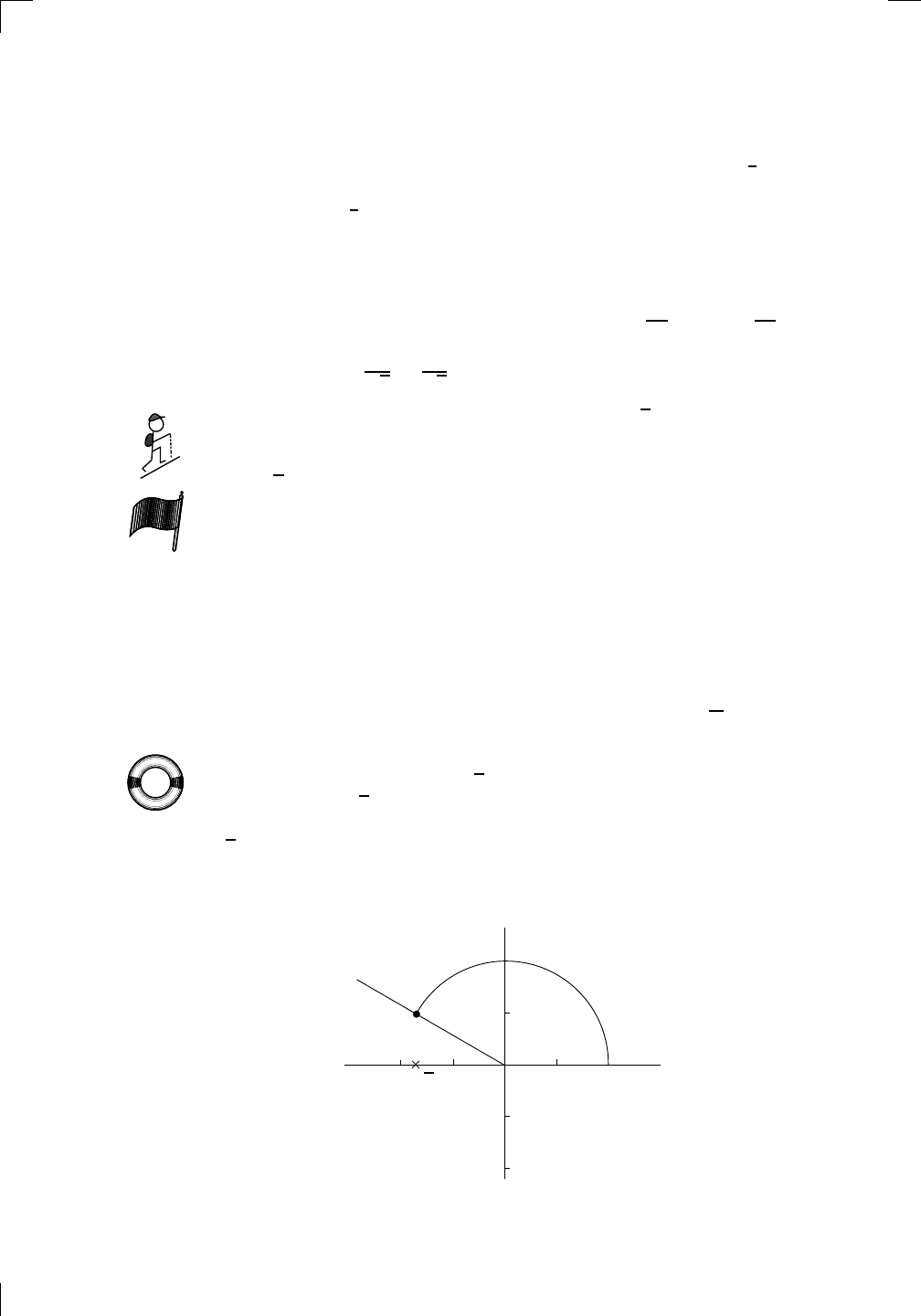
604 • Complex Numbers
2π-periodic in θ, however, so we can knock off any multiple of 2π from the
fraction 693π/4 and not affect the answer. So, write 693/4 = 173
1
4
. The
biggest even number less than this is 172, and the difference between these
two numbers is 173
1
4
−172 = 5/4. So, we can think of 693π/4 as 172π +5π/4.
Since 172π is a multiple of 2π (this is why we wanted an even number, 172
in this case), we know that e
i(693π/4)
= e
i(5π/4)
. That’s much nicer. Now we
can convert the whole thing to Cartesian form:
(1 − i)
99
= 2
99/2
e
i(693π/4)
= 2
99/2
e
i(5π/4)
= 2
99/2
cos
5π
4
+ i sin
5π
4
= 2
99/2
−
1
√
2
− i
1
√
2
.
In fact, this can be further simplified by writing 1/
√
2 as 2
−1/2
; the final
answer should be −2
49
(1 + i). Now, as an exercise, you should check that you
PSfrag replacements
(
a, b)
[
a, b]
(
a, b]
[
a, b)
(
a, ∞)
[
a, ∞)
(
−∞, b)
(
−∞, b]
(
−∞, ∞)
{
x : a < x < b}
{
x : a ≤ x ≤ b}
{
x : a < x ≤ b}
{
x : a ≤ x < b}
{
x : x ≥ a}
{
x : x > a}
{
x : x ≤ b}
{
x : x < b}
R
a
b
shadow
0
1
4
−
2
3
−
3
g(
x) = x
2
f(
x) = x
3
g(
x) = x
2
f(
x) = x
3
mirror (
y = x)
f
−
1
(x) =
3
√
x
y = h
(x)
y = h
−
1
(x)
y = (
x − 1)
2
−
1
x
Same height
−
x
Same length,
opposite signs
y = −
2x
−
2
1
y =
1
2
x − 1
2
−
1
y = 2
x
y = 10
x
y = 2
−
x
y = log
2
(
x)
4
3 units
mirror (
x-axis)
y = |
x|
y = |
log
2
(x)|
θ radians
θ units
30
◦
=
π
6
45
◦
=
π
4
60
◦
=
π
3
120
◦
=
2
π
3
135
◦
=
3
π
4
150
◦
=
5
π
6
90
◦
=
π
2
180
◦
= π
210
◦
=
7
π
6
225
◦
=
5
π
4
240
◦
=
4
π
3
270
◦
=
3
π
2
300
◦
=
5
π
3
315
◦
=
7
π
4
330
◦
=
11
π
6
0
◦
= 0 radians
θ
hyp
otenuse
opposite
adjacent
0 (
≡ 2π)
π
2
π
3
π
2
I
II
III
IV
θ
(
x, y)
x
y
r
7
π
6
reference angle
reference angle =
π
6
sin +
sin −
cos +
cos −
tan +
tan −
A
S
T
C
7
π
4
9
π
13
5
π
6
(this angle is
5
π
6
clockwise)
1
2
1
2
3
4
5
6
0
−
1
−
2
−
3
−
4
−
5
−
6
−
3π
−
5
π
2
−
2π
−
3
π
2
−
π
−
π
2
3
π
3
π
5
π
2
2
π
3
π
2
π
π
2
y = sin(
x)
1
0
−
1
−
3π
−
5
π
2
−
2π
−
3
π
2
−
π
−
π
2
3
π
5
π
2
2
π
2
π
3
π
2
π
π
2
y = sin(
x)
y = cos(
x)
−
π
2
π
2
y = tan(
x), −
π
2
< x <
π
2
0
−
π
2
π
2
y = tan(
x)
−
2π
−
3π
−
5
π
2
−
3
π
2
−
π
−
π
2
π
2
3
π
3
π
5
π
2
2
π
3
π
2
π
y = sec(
x)
y = csc(
x)
y = cot(
x)
y = f(
x)
−
1
1
2
y = g(
x)
3
y = h
(x)
4
5
−
2
f(
x) =
1
x
g(
x) =
1
x
2
etc.
0
1
π
1
2
π
1
3
π
1
4
π
1
5
π
1
6
π
1
7
π
g(
x) = sin
1
x
1
0
−
1
L
10
100
200
y =
π
2
y = −
π
2
y = tan
−
1
(x)
π
2
π
y =
sin(
x)
x
, x > 3
0
1
−
1
a
L
f(
x) = x sin (1/x)
(0 < x < 0
.3)
h
(x) = x
g(
x) = −x
a
L
lim
x
→a
+
f(x) = L
lim
x
→a
+
f(x) = ∞
lim
x
→a
+
f(x) = −∞
lim
x
→a
+
f(x) DNE
lim
x
→a
−
f(x) = L
lim
x
→a
−
f(x) = ∞
lim
x
→a
−
f(x) = −∞
lim
x
→a
−
f(x) DNE
M
}
lim
x
→a
−
f(x) = M
lim
x
→a
f(x) = L
lim
x
→a
f(x) DNE
lim
x
→∞
f(x) = L
lim
x
→∞
f(x) = ∞
lim
x
→∞
f(x) = −∞
lim
x
→∞
f(x) DNE
lim
x
→−∞
f(x) = L
lim
x
→−∞
f(x) = ∞
lim
x
→−∞
f(x) = −∞
lim
x
→−∞
f(x) DNE
lim
x →a
+
f(
x) = ∞
lim
x →a
+
f(
x) = −∞
lim
x →a
−
f(
x) = ∞
lim
x →a
−
f(
x) = −∞
lim
x →a
f(
x) = ∞
lim
x →a
f(
x) = −∞
lim
x →a
f(
x) DNE
y = f (
x)
a
y =
|
x|
x
1
−
1
y =
|
x + 2|
x + 2
1
−
1
−
2
1
2
3
4
a
a
b
y = x sin
1
x
y = x
y = −
x
a
b
c
d
C
a
b
c
d
−
1
0
1
2
3
time
y
t
u
(
t, f(t))
(
u, f(u))
time
y
t
u
y
x
(
x, f(x))
y = |
x|
(
z, f(z))
z
y = f(
x)
a
tangent at x = a
b
tangent at x = b
c
tangent at x = c
y = x
2
tangent
at x = −
1
u
v
uv
u + ∆
u
v + ∆
v
(
u + ∆u)(v + ∆v)
∆
u
∆
v
u
∆v
v∆
u
∆
u∆v
y = f(
x)
1
2
−
2
y = |
x
2
− 4|
y = x
2
− 4
y = −
2x + 5
y = g(
x)
1
2
3
4
5
6
7
8
9
0
−
1
−
2
−
3
−
4
−
5
−
6
y = f (
x)
3
−
3
3
−
3
0
−
1
2
easy
hard
flat
y = f
0
(
x)
3
−
3
0
−
1
2
1
−
1
y = sin(
x)
y = x
x
A
B
O
1
C
D
sin(
x)
tan(
x)
y =
sin(
x)
x
π
2
π
1
−
1
x = 0
a = 0
x > 0
a > 0
x < 0
a < 0
rest position
+
−
y = x
2
sin
1
x
N
A
B
H
a
b
c
O
H
A
B
C
D
h
r
R
θ
1000
2000
α
β
p
h
y = g(
x) = log
b
(x)
y = f(
x) = b
x
y = e
x
5
10
1
2
3
4
0
−
1
−
2
−
3
−
4
y = ln(
x)
y = cosh(
x)
y = sinh(
x)
y = tanh(
x)
y = sech(
x)
y = csch(
x)
y = coth(
x)
1
−
1
y = f(
x)
original function
inverse function
slope = 0 at (
x, y)
slope is infinite at (
y, x)
−
108
2
5
1
2
1
2
3
4
5
6
0
−
1
−
2
−
3
−
4
−
5
−
6
−
3π
−
5
π
2
−
2π
−
3
π
2
−
π
−
π
2
3
π
3
π
5
π
2
2
π
3
π
2
π
π
2
y = sin(
x)
1
0
−
1
−
3π
−
5
π
2
−
2π
−
3
π
2
−
π
−
π
2
3
π
5
π
2
2
π
2
π
3
π
2
π
π
2
y = sin(
x)
y = sin(
x), −
π
2
≤ x ≤
π
2
−
2
−
1
0
2
π
2
−
π
2
y = sin
−
1
(x)
y = cos(
x)
π
π
2
y = cos
−
1
(x)
−
π
2
1
x
α
β
y = tan(
x)
y = tan(
x)
1
y = tan
−
1
(x)
y = sec(
x)
y = sec
−
1
(x)
y = csc
−
1
(x)
y = cot
−
1
(x)
1
y = cosh
−
1
(x)
y = sinh
−
1
(x)
y = tanh
−
1
(x)
y = sech
−
1
(x)
y = csch
−
1
(x)
y = coth
−
1
(x)
(0
, 3)
(2
, −1)
(5
, 2)
(7
, 0)
(
−1, 44)
(0
, 1)
(1
, −12)
(2
, 305)
y = 1
2
(2
, 3)
y = f(
x)
y = g(
x)
a
b
c
a
b
c
s
c
0
c
1
(
a, f(a))
(
b, f(b))
1
2
1
2
3
4
5
6
0
−
1
−
2
−
3
−
4
−
5
−
6
−
3π
−
5
π
2
−
2π
−
3
π
2
−
π
−
π
2
3
π
3
π
5
π
2
2
π
3
π
2
π
π
2
y = sin(
x)
1
0
−
1
−
3π
−
5
π
2
−
2π
−
3
π
2
−
π
−
π
2
3
π
5
π
2
2
π
2
π
3
π
2
π
π
2
c
OR
Local maximum
Local minimum
Horizontal point of inflection
1
e
y = f
0
(
x)
y = f (
x) = x ln(x)
−
1
e
?
y = f(
x) = x
3
y = g(
x) = x
4
x
f(
x)
−
3
−
2
−
1
0
1
2
1
2
3
4
+
−
?
1
5
6
3
f
0
(
x)
2 −
1
2
√
6
2 +
1
2
√
6
f
00
(
x)
7
8
g
00
(
x)
f
00
(
x)
0
y =
(
x − 3)(x − 1)
2
x
3
(
x + 2)
y = x ln(
x)
1
e
−
1
e
5
−
108
2
α
β
2 −
1
2
√
6
2 +
1
2
√
6
y = x
2
(
x − 5)
3
−
e
−
1/2
√
3
e
−
1/2
√
3
−
e
−3/2
e
−
3/2
−
1
√
3
1
√
3
−
1
1
y = xe
−
3x
2
/2
y =
x
3
− 6
x
2
+ 13x − 8
x
28
2
600
500
400
300
200
100
0
−
100
−
200
−
300
−
400
−
500
−
600
0
10
−
10
5
−
5
20
−
20
15
−
15
0
4
5
6
x
P
0
(
x)
+
−
−
existing fence
new fence
enclosure
A
h
b
H
99
100
101
h
dA/dh
r
h
1
2
7
shallow
deep
LAND
SEA
N
y
z
s
t
3
11
9
L
(11)
√
11
y = L
(x)
y = f (
x)
11
y = L
(x)
y = f(
x)
F
P
a
a + ∆
x
f(
a + ∆x)
L
(a + ∆x)
f(
a)
error
df
∆
x
a
b
y = f(
x)
true zero
starting approximation
better approximation
v
t
3
5
50
40
60
4
20
30
25
t
1
t
2
t
3
t
4
t
n
−2
t
n
−1
t
0
= a
t
n
= b
v
1
v
2
v
3
v
4
v
n
−1
v
n
−
30
6
30
|
v|
a
b
p
q
c
v(
c)
v(
c
1
)
v(
c
2
)
v(
c
3
)
v(
c
4
)
v(
c
5
)
v(
c
6
)
t
1
t
2
t
3
t
4
t
5
c
1
c
2
c
3
c
4
c
5
c
6
t
0
=
a
t
6
=
b
t
16
=
b
t
10
=
b
a
b
x
y
y = f(
x)
1
2
y = x
5
0
−
2
y = 1
a
b
y = sin(
x)
π
−
π
0
−
1
−
2
0
2
4
y = x
2
0
1
2
3
4
2
n
4
n
6
n
2(
n−2)
n
2(
n−1)
n
2
n
n
= 2
width of each interval =
2
n
−
2
1
3
0
I
II
III
IV
4
y
dx
y = −
x
2
− 2x + 3
3
−
5
y = |−
x
2
− 2x + 3|
I
II
IIa
5
3
0
1
2
a
b
y = f (
x)
y = g(
x)
y = x
2
a
b
5
3
0
1
2
y =
√
x
2
√
2
2
2
dy
x
2
a
b
y = f(
x)
y = g(
x)
M
m
1
2
−
1
−
2
0
y = e
−
x
2
1
2
e
−
1/4
f
av
y = f
av
c
A
M
0
1
2
a
b
x
t
y = f (
t)
F (
x )
y = f (
t)
F (
x + h)
x + h
F (
x + h) − F (x)
f(
x)
1
2
y = sin(
x)
π
−
π
−
1
−
2
y =
1
x
y = x
2
1
2
1
−
1
y = ln
|x|
θ
a
x
a
x
p
a
2
− x
2
3
x
p
9 − x
2
p
x
2
+ a
2
x
a
p
x
2
+ 15
x
√
15
x
p
x
2
− a
2
a
x
p
x
2
− 4
2
x
−
p
x
2
− a
2
a
x
−
p
x
2
− 4
2
y = f(
x)
a
b
a + ε
ε
Z
b
a
+ε
f(x) dx
small
even smaller
y = g(
x)
infinite area
finite area
1
y =
1
x
y =
1
x
p
, p < 1 (typical)
y =
1
x
p
, p > 1 (typical)
a
1
a
2
a
3
a
4
a
5
a
6
a
7
a
8
1
2
3
4
5
6
7
8
n
a
n
x
y
y = f(
x)
(
a, f(a))
a
−
1
0
1
a
6
1
2
7
1
2
7
?
−
2
−
1
−
2
t = 0
t = π/
6
t = π/
4
t = π/
3
t = π/
2
3
0
t = −
2
t = −
3/2
t = ±
1
t = −
1/2
t = 0
t = 1
/2
t = 3
/2
t = 2
12
−
12
θ
r
P
θ
r
P
11
π
6
2
(
−1, −1)
wrong point
π
4
5
π
4
√
2
(0
, 1)
(0
, −3)
(
−2, 0)
π
2
3
π
2
π
r = 3 sin(
θ)
3
π
2
θ
2
π
1
0
−
1
−
2
−
3
0
3
2
−
3
2
0
r = 1 + 2 cos(θ)
2π
3
4π
3
0
π
0
pi
−
3
2
3π
2
1
2
3
0
−1
−2
−3
0 ≤ θ ≤
2π
3
0 ≤ θ ≤ π
0 ≤ θ ≤ 2π
r = 1 + cos(θ)
r = 1 +
3
4
cos(θ)
−
1
4
r = sin(2θ)
r = sin(3θ)
r =
1
π
θ
0 ≤ θ ≤ 4π
r =
2
1 + sin(θ)
−
π
4
≤ θ ≤
5π
4
0 ≤ θ ≤ 2π
0 ≤ θ ≤ π
−4
−5
4
5
f(θ)
f(θ + dθ)
θ
dθ
θ + dθ
approximating region
exact region
0 ≤ θ ≤ 2π
r = |1 + 2 cos(θ)|
2i
2 − 3i
−1
θ = 0
θ =
π
4
θ =
π
2
θ =
2π
3
θ = π
θ =
13π
12
θ =
3π
2
θ =
7π
4
1 = e
0
e
i
π
4
i = e
i
π
2
e
i
2π
3
−1 = e
iπ
e
i
13π
12
−i = e
i
3π
2
e
i
7π
4
i
−i
1
θ
1 − i
2i
−2i
2
−2
6i
−6i
6
−6
can arrive at the same answer by starting off using an alternate polar form,
1 − i =
√
2e
−iπ/4
.
In summary, to take a large power of a complex number, first convert it to
PSfrag replacements
(
a, b)
[
a, b]
(
a, b]
[
a, b)
(
a, ∞)
[
a, ∞)
(
−∞, b)
(
−∞, b]
(
−∞, ∞)
{
x : a < x < b}
{
x : a ≤ x ≤ b}
{
x : a < x ≤ b}
{
x : a ≤ x < b}
{
x : x ≥ a}
{
x : x > a}
{
x : x ≤ b}
{
x : x < b}
R
a
b
shadow
0
1
4
−
2
3
−
3
g(
x) = x
2
f(
x) = x
3
g(
x) = x
2
f(
x) = x
3
mirror (
y = x)
f
−
1
(x) =
3
√
x
y = h
(x)
y = h
−
1
(x)
y = (
x − 1)
2
−
1
x
Same height
−
x
Same length,
opposite signs
y = −
2x
−
2
1
y =
1
2
x − 1
2
−
1
y = 2
x
y = 10
x
y = 2
−
x
y = log
2
(
x)
4
3 units
mirror (
x-axis)
y = |
x|
y = |
log
2
(x)|
θ radians
θ units
30
◦
=
π
6
45
◦
=
π
4
60
◦
=
π
3
120
◦
=
2
π
3
135
◦
=
3
π
4
150
◦
=
5
π
6
90
◦
=
π
2
180
◦
= π
210
◦
=
7
π
6
225
◦
=
5
π
4
240
◦
=
4
π
3
270
◦
=
3
π
2
300
◦
=
5
π
3
315
◦
=
7
π
4
330
◦
=
11
π
6
0
◦
= 0 radians
θ
hyp
otenuse
opposite
adjacent
0 (
≡ 2π)
π
2
π
3
π
2
I
II
III
IV
θ
(
x, y)
x
y
r
7
π
6
reference angle
reference angle =
π
6
sin +
sin −
cos +
cos −
tan +
tan −
A
S
T
C
7
π
4
9
π
13
5
π
6
(this angle is
5
π
6
clockwise)
1
2
1
2
3
4
5
6
0
−
1
−
2
−
3
−
4
−
5
−
6
−
3π
−
5
π
2
−
2π
−
3
π
2
−
π
−
π
2
3
π
3
π
5
π
2
2
π
3
π
2
π
π
2
y = sin(
x)
1
0
−
1
−
3π
−
5
π
2
−
2π
−
3
π
2
−
π
−
π
2
3
π
5
π
2
2
π
2
π
3
π
2
π
π
2
y = sin(
x)
y = cos(
x)
−
π
2
π
2
y = tan(
x), −
π
2
< x <
π
2
0
−
π
2
π
2
y = tan(
x)
−
2π
−
3π
−
5
π
2
−
3
π
2
−
π
−
π
2
π
2
3
π
3
π
5
π
2
2
π
3
π
2
π
y = sec(
x)
y = csc(
x)
y = cot(
x)
y = f (
x)
−
1
1
2
y = g(
x)
3
y = h
(x)
4
5
−
2
f(
x) =
1
x
g(
x) =
1
x
2
etc.
0
1
π
1
2
π
1
3
π
1
4
π
1
5
π
1
6
π
1
7
π
g(
x) = sin
1
x
1
0
−
1
L
10
100
200
y =
π
2
y = −
π
2
y = tan
−
1
(x)
π
2
π
y =
sin(
x)
x
, x > 3
0
1
−
1
a
L
f(
x) = x sin (1/x)
(0 < x < 0
.3)
h
(x) = x
g(
x) = −x
a
L
lim
x
→a
+
f(x) = L
lim
x
→a
+
f(x) = ∞
lim
x
→a
+
f(x) = −∞
lim
x
→a
+
f(x) DNE
lim
x
→a
−
f(x) = L
lim
x
→a
−
f(x) = ∞
lim
x
→a
−
f(x) = −∞
lim
x
→a
−
f(x) DNE
M
}
lim
x
→a
−
f(x) = M
lim
x
→a
f(x) = L
lim
x
→a
f(x) DNE
lim
x
→∞
f(x) = L
lim
x
→∞
f(x) = ∞
lim
x
→∞
f(x) = −∞
lim
x
→∞
f(x) DNE
lim
x
→−∞
f(x) = L
lim
x
→−∞
f(x) = ∞
lim
x
→−∞
f(x) = −∞
lim
x
→−∞
f(x) DNE
lim
x →a
+
f(
x) = ∞
lim
x →a
+
f(
x) = −∞
lim
x →a
−
f(
x) = ∞
lim
x →a
−
f(
x) = −∞
lim
x →a
f(
x) = ∞
lim
x →a
f(
x) = −∞
lim
x →a
f(
x) DNE
y = f (
x)
a
y =
|
x|
x
1
−
1
y =
|
x + 2|
x + 2
1
−
1
−
2
1
2
3
4
a
a
b
y = x sin
1
x
y = x
y = −
x
a
b
c
d
C
a
b
c
d
−
1
0
1
2
3
time
y
t
u
(
t, f(t))
(
u, f(u))
time
y
t
u
y
x
(
x, f(x))
y = |
x|
(
z, f(z))
z
y = f (
x)
a
tangent at x = a
b
tangent at x = b
c
tangent at x = c
y = x
2
tangent
at x = −
1
u
v
uv
u + ∆
u
v + ∆
v
(
u + ∆u)(v + ∆v)
∆
u
∆
v
u
∆v
v∆
u
∆
u∆v
y = f (
x)
1
2
−
2
y = |
x
2
− 4|
y = x
2
− 4
y = −
2x + 5
y = g(
x)
1
2
3
4
5
6
7
8
9
0
−
1
−
2
−
3
−
4
−
5
−
6
y = f (
x)
3
−
3
3
−
3
0
−
1
2
easy
hard
flat
y = f
0
(
x)
3
−
3
0
−
1
2
1
−
1
y = sin(
x)
y = x
x
A
B
O
1
C
D
sin(
x)
tan(
x)
y =
sin(
x)
x
π
2
π
1
−
1
x = 0
a = 0
x > 0
a > 0
x < 0
a < 0
rest position
+
−
y = x
2
sin
1
x
N
A
B
H
a
b
c
O
H
A
B
C
D
h
r
R
θ
1000
2000
α
β
p
h
y = g(
x) = log
b
(x)
y = f (
x) = b
x
y = e
x
5
10
1
2
3
4
0
−
1
−
2
−
3
−
4
y = ln(
x)
y = cosh(
x)
y = sinh(
x)
y = tanh(
x)
y = sech(
x)
y = csch(
x)
y = coth(
x)
1
−
1
y = f (
x)
original function
inverse function
slope = 0 at (
x, y)
slope is infinite at (
y, x)
−
108
2
5
1
2
1
2
3
4
5
6
0
−
1
−
2
−
3
−
4
−
5
−
6
−
3π
−
5
π
2
−
2π
−
3
π
2
−
π
−
π
2
3
π
3
π
5
π
2
2
π
3
π
2
π
π
2
y = sin(
x)
1
0
−
1
−
3π
−
5
π
2
−
2π
−
3
π
2
−
π
−
π
2
3
π
5
π
2
2
π
2
π
3
π
2
π
π
2
y = sin(
x)
y = sin(
x), −
π
2
≤ x ≤
π
2
−
2
−
1
0
2
π
2
−
π
2
y = sin
−
1
(x)
y = cos(
x)
π
π
2
y = cos
−
1
(x)
−
π
2
1
x
α
β
y = tan(
x)
y = tan(
x)
1
y = tan
−
1
(x)
y = sec(
x)
y = sec
−
1
(x)
y = csc
−
1
(x)
y = cot
−
1
(x)
1
y = cosh
−
1
(x)
y = sinh
−
1
(x)
y = tanh
−
1
(x)
y = sech
−
1
(x)
y = csch
−
1
(x)
y = coth
−
1
(x)
(0
, 3)
(2
, −1)
(5
, 2)
(7
, 0)
(
−1, 44)
(0
, 1)
(1
, −12)
(2
, 305)
y = 1
2
(2
, 3)
y = f (
x)
y = g(
x)
a
b
c
a
b
c
s
c
0
c
1
(
a, f(a))
(
b, f(b))
1
2
1
2
3
4
5
6
0
−
1
−
2
−
3
−
4
−
5
−
6
−
3π
−
5
π
2
−
2π
−
3
π
2
−
π
−
π
2
3
π
3
π
5
π
2
2
π
3
π
2
π
π
2
y = sin(
x)
1
0
−
1
−
3π
−
5
π
2
−
2π
−
3
π
2
−
π
−
π
2
3
π
5
π
2
2
π
2
π
3
π
2
π
π
2
c
OR
Local maximum
Local minimum
Horizontal point of inflection
1
e
y = f
0
(
x)
y = f(
x) = x ln(x)
−
1
e
?
y = f(
x) = x
3
y = g(
x) = x
4
x
f(
x)
−
3
−
2
−
1
0
1
2
1
2
3
4
+
−
?
1
5
6
3
f
0
(
x)
2 −
1
2
√
6
2 +
1
2
√
6
f
00
(
x)
7
8
g
00
(
x)
f
00
(
x)
0
y =
(
x − 3)(x − 1)
2
x
3
(
x + 2)
y = x ln(
x)
1
e
−
1
e
5
−
108
2
α
β
2 −
1
2
√
6
2 +
1
2
√
6
y = x
2
(
x − 5)
3
−
e
−
1/2
√
3
e
−
1/2
√
3
−
e
−3/2
e
−
3/2
−
1
√
3
1
√
3
−
1
1
y = xe
−
3x
2
/2
y =
x
3
− 6
x
2
+ 13x − 8
x
28
2
600
500
400
300
200
100
0
−
100
−
200
−
300
−
400
−
500
−
600
0
10
−
10
5
−
5
20
−
20
15
−
15
0
4
5
6
x
P
0
(
x)
+
−
−
existing fence
new fence
enclosure
A
h
b
H
99
100
101
h
dA/dh
r
h
1
2
7
shallow
deep
LAND
SEA
N
y
z
s
t
3
11
9
L
(11)
√
11
y = L
(x)
y = f (
x)
11
y = L
(x)
y = f (
x)
F
P
a
a + ∆
x
f(
a + ∆x)
L
(a + ∆x)
f(
a)
error
df
∆
x
a
b
y = f (
x)
true zero
starting approximation
better approximation
v
t
3
5
50
40
60
4
20
30
25
t
1
t
2
t
3
t
4
t
n
−2
t
n
−1
t
0
= a
t
n
= b
v
1
v
2
v
3
v
4
v
n
−1
v
n
−
30
6
30
|
v|
a
b
p
q
c
v(
c)
v(
c
1
)
v(
c
2
)
v(
c
3
)
v(
c
4
)
v(
c
5
)
v(
c
6
)
t
1
t
2
t
3
t
4
t
5
c
1
c
2
c
3
c
4
c
5
c
6
t
0
=
a
t
6
=
b
t
16
=
b
t
10
=
b
a
b
x
y
y = f (
x)
1
2
y = x
5
0
−
2
y = 1
a
b
y = sin(
x)
π
−
π
0
−
1
−
2
0
2
4
y = x
2
0
1
2
3
4
2
n
4
n
6
n
2(
n−2)
n
2(
n−1)
n
2
n
n
= 2
width of each interval =
2
n
−
2
1
3
0
I
II
III
IV
4
y
dx
y = −
x
2
− 2x + 3
3
−
5
y = |−
x
2
− 2x + 3|
I
II
IIa
5
3
0
1
2
a
b
y = f (
x)
y = g(
x)
y = x
2
a
b
5
3
0
1
2
y =
√
x
2
√
2
2
2
dy
x
2
a
b
y = f (
x)
y = g(
x)
M
m
1
2
−
1
−
2
0
y = e
−
x
2
1
2
e
−
1/4
f
av
y = f
av
c
A
M
0
1
2
a
b
x
t
y = f(
t)
F (
x )
y = f(
t)
F (
x + h )
x + h
F (
x + h) − F (x)
f(
x)
1
2
y = sin(
x)
π
−
π
−
1
−
2
y =
1
x
y = x
2
1
2
1
−
1
y = ln
|x|
θ
a
x
a
x
p
a
2
− x
2
3
x
p
9 − x
2
p
x
2
+ a
2
x
a
p
x
2
+ 15
x
√
15
x
p
x
2
− a
2
a
x
p
x
2
− 4
2
x
−
p
x
2
− a
2
a
x
−
p
x
2
− 4
2
y = f (
x)
a
b
a + ε
ε
Z
b
a
+ε
f(x) dx
small
even smaller
y = g(
x)
infinite area
finite area
1
y =
1
x
y =
1
x
p
, p < 1 (typical)
y =
1
x
p
, p > 1 (typical)
a
1
a
2
a
3
a
4
a
5
a
6
a
7
a
8
1
2
3
4
5
6
7
8
n
a
n
x
y
y = f (
x)
(
a, f(a))
a
−
1
0
1
a
6
1
2
7
1
2
7
?
−
2
−
1
−
2
t = 0
t = π/
6
t = π/
4
t = π/
3
t = π/
2
3
0
t = −
2
t = −
3/2
t = ±
1
t = −
1/2
t = 0
t = 1
/2
t = 3
/2
t = 2
12
−
12
θ
r
P
θ
r
P
11
π
6
2
(
−1, −1)
wrong point
π
4
5
π
4
√
2
(0
, 1)
(0
, −3)
(
−2, 0)
π
2
3
π
2
π
r = 3 sin(
θ)
3
π
2
θ
2
π
1
0
−1
−2
−3
0
3
2
−
3
2
0
r = 1 + 2 cos(θ)
2π
3
4π
3
0
π
0
pi
−
3
2
3π
2
1
2
3
0
−1
−2
−3
0 ≤ θ ≤
2π
3
0 ≤ θ ≤ π
0 ≤ θ ≤ 2π
r = 1 + cos(θ)
r = 1 +
3
4
cos(θ)
−
1
4
r = sin(2θ)
r = sin(3θ)
r =
1
π
θ
0 ≤ θ ≤ 4π
r =
2
1 + sin(θ)
−
π
4
≤ θ ≤
5π
4
0 ≤ θ ≤ 2π
0 ≤ θ ≤ π
−4
−5
4
5
f(θ)
f(θ + dθ)
θ
dθ
θ + dθ
approximating region
exact region
0 ≤ θ ≤ 2π
r = |1 + 2 cos(θ)|
2i
2 − 3i
−1
θ = 0
θ =
π
4
θ =
π
2
θ =
2π
3
θ = π
θ =
13π
12
θ =
3π
2
θ =
7π
4
1 = e
0
e
i
π
4
i = e
i
π
2
e
i
2π
3
−1 = e
iπ
e
i
13π
12
−i = e
i
3π
2
e
i
7π
4
i
−i
1
θ
1 − i
2i
−2i
2
−2
6i
−6i
6
−6
polar form, then take the power. Find the largest even multiple of π less than
the angle θ, and take that away from θ and replace θ by that new number.
Finally, convert back to Cartesian form.
28.4 Solving z
n
= w
Let’s move onto a trickier subject: how to solve equations of the form z
n
= w,
where n is a given integer and w is a given complex number. This amounts
to taking nth roots of w, but we don’t just want to say z =
n
√
w since that
doesn’t tell us very much. Instead, we’ll try to find a solution directly. Since
powers work so well in polar form, that’s what we’ll use.
For example, to solve z
5
= −
√
3 + i, we should use polar coordinates for
PSfrag replacements
(
a, b)
[
a, b]
(
a, b]
[
a, b)
(
a, ∞)
[
a, ∞)
(
−∞, b)
(
−∞, b]
(
−∞, ∞)
{
x : a < x < b}
{
x : a ≤ x ≤ b}
{
x : a < x ≤ b}
{
x : a ≤ x < b}
{
x : x ≥ a}
{
x : x > a}
{
x : x ≤ b}
{
x : x < b}
R
a
b
shadow
0
1
4
−
2
3
−
3
g(
x) = x
2
f(
x) = x
3
g(
x) = x
2
f(
x) = x
3
mirror (
y = x)
f
−
1
(x) =
3
√
x
y = h
(x)
y = h
−
1
(x)
y = (
x − 1)
2
−
1
x
Same height
−
x
Same length,
opposite signs
y = −
2x
−
2
1
y =
1
2
x − 1
2
−
1
y = 2
x
y = 10
x
y = 2
−
x
y = log
2
(
x)
4
3 units
mirror (
x-axis)
y = |
x|
y = |
log
2
(x)|
θ radians
θ units
30
◦
=
π
6
45
◦
=
π
4
60
◦
=
π
3
120
◦
=
2
π
3
135
◦
=
3
π
4
150
◦
=
5
π
6
90
◦
=
π
2
180
◦
= π
210
◦
=
7
π
6
225
◦
=
5
π
4
240
◦
=
4
π
3
270
◦
=
3
π
2
300
◦
=
5
π
3
315
◦
=
7
π
4
330
◦
=
11
π
6
0
◦
= 0 radians
θ
hyp
otenuse
opposite
adjacent
0 (
≡ 2π)
π
2
π
3
π
2
I
II
III
IV
θ
(
x, y)
x
y
r
7
π
6
reference angle
reference angle =
π
6
sin +
sin −
cos +
cos −
tan +
tan −
A
S
T
C
7
π
4
9
π
13
5
π
6
(this angle is
5
π
6
clockwise)
1
2
1
2
3
4
5
6
0
−
1
−
2
−
3
−
4
−
5
−
6
−
3π
−
5
π
2
−
2π
−
3
π
2
−
π
−
π
2
3
π
3
π
5
π
2
2
π
3
π
2
π
π
2
y = sin(
x)
1
0
−
1
−
3π
−
5
π
2
−
2π
−
3
π
2
−
π
−
π
2
3
π
5
π
2
2
π
2
π
3
π
2
π
π
2
y = sin(
x)
y = cos(
x)
−
π
2
π
2
y = tan(
x), −
π
2
< x <
π
2
0
−
π
2
π
2
y = tan(
x)
−
2π
−
3π
−
5
π
2
−
3
π
2
−
π
−
π
2
π
2
3
π
3
π
5
π
2
2
π
3
π
2
π
y = sec(
x)
y = csc(
x)
y = cot(
x)
y = f(
x)
−
1
1
2
y = g(
x)
3
y = h
(x)
4
5
−
2
f(
x) =
1
x
g(
x) =
1
x
2
etc.
0
1
π
1
2
π
1
3
π
1
4
π
1
5
π
1
6
π
1
7
π
g(
x) = sin
1
x
1
0
−
1
L
10
100
200
y =
π
2
y = −
π
2
y = tan
−
1
(x)
π
2
π
y =
sin(
x)
x
, x > 3
0
1
−
1
a
L
f(
x) = x sin (1/x)
(0 < x < 0
.3)
h
(x) = x
g(
x) = −x
a
L
lim
x
→a
+
f(x) = L
lim
x
→a
+
f(x) = ∞
lim
x
→a
+
f(x) = −∞
lim
x
→a
+
f(x) DNE
lim
x
→a
−
f(x) = L
lim
x
→a
−
f(x) = ∞
lim
x
→a
−
f(x) = −∞
lim
x
→a
−
f(x) DNE
M
}
lim
x
→a
−
f(x) = M
lim
x
→a
f(x) = L
lim
x
→a
f(x) DNE
lim
x
→∞
f(x) = L
lim
x
→∞
f(x) = ∞
lim
x
→∞
f(x) = −∞
lim
x
→∞
f(x) DNE
lim
x
→−∞
f(x) = L
lim
x
→−∞
f(x) = ∞
lim
x
→−∞
f(x) = −∞
lim
x
→−∞
f(x) DNE
lim
x →a
+
f(
x) = ∞
lim
x →a
+
f(
x) = −∞
lim
x →a
−
f(
x) = ∞
lim
x →a
−
f(
x) = −∞
lim
x →a
f(
x) = ∞
lim
x →a
f(
x) = −∞
lim
x →a
f(
x) DNE
y = f (
x)
a
y =
|
x|
x
1
−
1
y =
|
x + 2|
x + 2
1
−
1
−
2
1
2
3
4
a
a
b
y = x sin
1
x
y = x
y = −
x
a
b
c
d
C
a
b
c
d
−
1
0
1
2
3
time
y
t
u
(
t, f(t))
(
u, f(u))
time
y
t
u
y
x
(
x, f(x))
y = |
x|
(
z, f(z))
z
y = f(
x)
a
tangent at x = a
b
tangent at x = b
c
tangent at x = c
y = x
2
tangent
at x = −
1
u
v
uv
u + ∆
u
v + ∆
v
(
u + ∆u)(v + ∆v)
∆
u
∆
v
u
∆v
v∆
u
∆
u∆v
y = f(
x)
1
2
−
2
y = |
x
2
− 4|
y = x
2
− 4
y = −
2x + 5
y = g(
x)
1
2
3
4
5
6
7
8
9
0
−
1
−
2
−
3
−
4
−
5
−
6
y = f (
x)
3
−
3
3
−
3
0
−
1
2
easy
hard
flat
y = f
0
(
x)
3
−
3
0
−
1
2
1
−
1
y = sin(
x)
y = x
x
A
B
O
1
C
D
sin(
x)
tan(
x)
y =
sin(
x)
x
π
2
π
1
−
1
x = 0
a = 0
x > 0
a > 0
x < 0
a < 0
rest position
+
−
y = x
2
sin
1
x
N
A
B
H
a
b
c
O
H
A
B
C
D
h
r
R
θ
1000
2000
α
β
p
h
y = g(
x) = log
b
(x)
y = f(
x) = b
x
y = e
x
5
10
1
2
3
4
0
−
1
−
2
−
3
−
4
y = ln(
x)
y = cosh(
x)
y = sinh(
x)
y = tanh(
x)
y = sech(
x)
y = csch(
x)
y = coth(
x)
1
−
1
y = f(
x)
original function
inverse function
slope = 0 at (
x, y)
slope is infinite at (
y, x)
−
108
2
5
1
2
1
2
3
4
5
6
0
−
1
−
2
−
3
−
4
−
5
−
6
−
3π
−
5
π
2
−
2π
−
3
π
2
−
π
−
π
2
3
π
3
π
5
π
2
2
π
3
π
2
π
π
2
y = sin(
x)
1
0
−
1
−
3π
−
5
π
2
−
2π
−
3
π
2
−
π
−
π
2
3
π
5
π
2
2
π
2
π
3
π
2
π
π
2
y = sin(
x)
y = sin(
x), −
π
2
≤ x ≤
π
2
−
2
−
1
0
2
π
2
−
π
2
y = sin
−
1
(x)
y = cos(
x)
π
π
2
y = cos
−
1
(x)
−
π
2
1
x
α
β
y = tan(
x)
y = tan(
x)
1
y = tan
−
1
(x)
y = sec(
x)
y = sec
−
1
(x)
y = csc
−
1
(x)
y = cot
−
1
(x)
1
y = cosh
−
1
(x)
y = sinh
−
1
(x)
y = tanh
−
1
(x)
y = sech
−
1
(x)
y = csch
−
1
(x)
y = coth
−
1
(x)
(0
, 3)
(2
, −1)
(5
, 2)
(7
, 0)
(
−1, 44)
(0
, 1)
(1
, −12)
(2
, 305)
y = 1
2
(2
, 3)
y = f(
x)
y = g(
x)
a
b
c
a
b
c
s
c
0
c
1
(
a, f(a))
(
b, f(b))
1
2
1
2
3
4
5
6
0
−
1
−
2
−
3
−
4
−
5
−
6
−
3π
−
5
π
2
−
2π
−
3
π
2
−
π
−
π
2
3
π
3
π
5
π
2
2
π
3
π
2
π
π
2
y = sin(
x)
1
0
−
1
−
3π
−
5
π
2
−
2π
−
3
π
2
−
π
−
π
2
3
π
5
π
2
2
π
2
π
3
π
2
π
π
2
c
OR
Local maximum
Local minimum
Horizontal point of inflection
1
e
y = f
0
(
x)
y = f (
x) = x ln(x)
−
1
e
?
y = f(
x) = x
3
y = g(
x) = x
4
x
f(
x)
−
3
−
2
−
1
0
1
2
1
2
3
4
+
−
?
1
5
6
3
f
0
(
x)
2 −
1
2
√
6
2 +
1
2
√
6
f
00
(
x)
7
8
g
00
(
x)
f
00
(
x)
0
y =
(
x − 3)(x − 1)
2
x
3
(
x + 2)
y = x ln(
x)
1
e
−
1
e
5
−
108
2
α
β
2 −
1
2
√
6
2 +
1
2
√
6
y = x
2
(
x − 5)
3
−
e
−
1/2
√
3
e
−
1/2
√
3
−
e
−3/2
e
−
3/2
−
1
√
3
1
√
3
−
1
1
y = xe
−
3x
2
/2
y =
x
3
− 6
x
2
+ 13x − 8
x
28
2
600
500
400
300
200
100
0
−
100
−
200
−
300
−
400
−
500
−
600
0
10
−
10
5
−
5
20
−
20
15
−
15
0
4
5
6
x
P
0
(
x)
+
−
−
existing fence
new fence
enclosure
A
h
b
H
99
100
101
h
dA/dh
r
h
1
2
7
shallow
deep
LAND
SEA
N
y
z
s
t
3
11
9
L
(11)
√
11
y = L
(x)
y = f (
x)
11
y = L
(x)
y = f(
x)
F
P
a
a + ∆
x
f(
a + ∆x)
L
(a + ∆x)
f(
a)
error
df
∆
x
a
b
y = f(
x)
true zero
starting approximation
better approximation
v
t
3
5
50
40
60
4
20
30
25
t
1
t
2
t
3
t
4
t
n
−2
t
n
−1
t
0
= a
t
n
= b
v
1
v
2
v
3
v
4
v
n
−1
v
n
−
30
6
30
|
v|
a
b
p
q
c
v(
c)
v(
c
1
)
v(
c
2
)
v(
c
3
)
v(
c
4
)
v(
c
5
)
v(
c
6
)
t
1
t
2
t
3
t
4
t
5
c
1
c
2
c
3
c
4
c
5
c
6
t
0
=
a
t
6
=
b
t
16
=
b
t
10
=
b
a
b
x
y
y = f(
x)
1
2
y = x
5
0
−
2
y = 1
a
b
y = sin(
x)
π
−
π
0
−
1
−
2
0
2
4
y = x
2
0
1
2
3
4
2
n
4
n
6
n
2(
n−2)
n
2(
n−1)
n
2
n
n
= 2
width of each interval =
2
n
−
2
1
3
0
I
II
III
IV
4
y
dx
y = −
x
2
− 2x + 3
3
−
5
y = |−
x
2
− 2x + 3|
I
II
IIa
5
3
0
1
2
a
b
y = f (
x)
y = g(
x)
y = x
2
a
b
5
3
0
1
2
y =
√
x
2
√
2
2
2
dy
x
2
a
b
y = f(
x)
y = g(
x)
M
m
1
2
−
1
−
2
0
y = e
−
x
2
1
2
e
−
1/4
f
av
y = f
av
c
A
M
0
1
2
a
b
x
t
y = f (
t)
F (
x )
y = f (
t)
F (
x + h)
x + h
F (
x + h) − F (x)
f(
x)
1
2
y = sin(
x)
π
−
π
−
1
−
2
y =
1
x
y = x
2
1
2
1
−
1
y = ln
|x|
θ
a
x
a
x
p
a
2
− x
2
3
x
p
9 − x
2
p
x
2
+ a
2
x
a
p
x
2
+ 15
x
√
15
x
p
x
2
− a
2
a
x
p
x
2
− 4
2
x
−
p
x
2
− a
2
a
x
−
p
x
2
− 4
2
y = f(
x)
a
b
a + ε
ε
Z
b
a
+ε
f(x) dx
small
even smaller
y = g(
x)
infinite area
finite area
1
y =
1
x
y =
1
x
p
, p < 1 (typical)
y =
1
x
p
, p > 1 (typical)
a
1
a
2
a
3
a
4
a
5
a
6
a
7
a
8
1
2
3
4
5
6
7
8
n
a
n
x
y
y = f(
x)
(
a, f(a))
a
−
1
0
1
a
6
1
2
7
1
2
7
?
−
2
−
1
−
2
t = 0
t = π/
6
t = π/
4
t = π/
3
t = π/
2
3
0
t = −
2
t = −
3/2
t = ±
1
t = −
1/2
t = 0
t = 1
/2
t = 3
/2
t = 2
12
−
12
θ
r
P
θ
r
P
11
π
6
2
(
−1, −1)
wrong point
π
4
5
π
4
√
2
(0, 1)
(0, −3)
(−2, 0)
π
2
3π
2
π
r = 3 sin(θ)
3π
2
θ
2π
1
0
−1
−2
−3
0
3
2
−
3
2
0
r = 1 + 2 cos(θ)
2π
3
4π
3
0
π
0
pi
−
3
2
3π
2
1
2
3
0
−1
−2
−3
0 ≤ θ ≤
2π
3
0 ≤ θ ≤ π
0 ≤ θ ≤ 2π
r = 1 + cos(θ)
r = 1 +
3
4
cos(θ)
−
1
4
r = sin(2θ)
r = sin(3θ)
r =
1
π
θ
0 ≤ θ ≤ 4π
r =
2
1 + sin(θ)
−
π
4
≤ θ ≤
5π
4
0 ≤ θ ≤ 2π
0 ≤ θ ≤ π
−4
−5
4
5
f(θ)
f(θ + dθ)
θ
dθ
θ + dθ
approximating region
exact region
0 ≤ θ ≤ 2π
r = |1 + 2 cos(θ)|
2i
2 − 3i
−1
θ = 0
θ =
π
4
θ =
π
2
θ =
2π
3
θ = π
θ =
13π
12
θ =
3π
2
θ =
7π
4
1 = e
0
e
i
π
4
i = e
i
π
2
e
i
2π
3
−1 = e
iπ
e
i
13π
12
−i = e
i
3π
2
e
i
7π
4
i
−i
1
θ
1 − i
2i
−2i
2
−2
6i
−6i
6
−6
both z and w = −
√
3 + i. Since we don’t know what z is, let’s put z = re
iθ
.
Now to find z, we just have to find what r and θ are. As for w, let’s write
−
√
3 + i = Re
iϕ
and then find R and ϕ. (We have to use R and ϕ instead of
r and θ since the last two variables are already taken for z.) Now, let’s draw
a picture of the situation:
PSfrag replacements
(
a, b)
[
a, b]
(
a, b]
[
a, b)
(
a, ∞)
[
a, ∞)
(
−∞, b)
(
−∞, b]
(
−∞, ∞)
{
x : a < x < b}
{
x : a ≤ x ≤ b}
{
x : a < x ≤ b}
{
x : a ≤ x < b}
{
x : x ≥ a}
{
x : x > a}
{
x : x ≤ b}
{
x : x < b}
R
a
b
shadow
0
1
4
−
2
3
−
3
g(
x) = x
2
f(
x) = x
3
g(
x) = x
2
f(
x) = x
3
mirror (
y = x)
f
−
1
(x) =
3
√
x
y = h
(x)
y = h
−
1
(x)
y = (
x − 1)
2
−
1
x
Same height
−
x
Same length,
opposite signs
y = −
2x
−
2
1
y =
1
2
x − 1
2
−
1
y = 2
x
y = 10
x
y = 2
−
x
y = log
2
(
x)
4
3 units
mirror (
x-axis)
y = |
x|
y = |
log
2
(x)|
θ radians
θ units
30
◦
=
π
6
45
◦
=
π
4
60
◦
=
π
3
120
◦
=
2
π
3
135
◦
=
3
π
4
150
◦
=
5
π
6
90
◦
=
π
2
180
◦
= π
210
◦
=
7
π
6
225
◦
=
5
π
4
240
◦
=
4
π
3
270
◦
=
3
π
2
300
◦
=
5
π
3
315
◦
=
7
π
4
330
◦
=
11
π
6
0
◦
= 0 radians
θ
hyp
otenuse
opposite
adjacent
0 (
≡ 2π)
π
2
π
3
π
2
I
II
III
IV
θ
(
x, y)
x
y
r
7
π
6
reference angle
reference angle =
π
6
sin +
sin −
cos +
cos −
tan +
tan −
A
S
T
C
7
π
4
9
π
13
5
π
6
(this angle is
5
π
6
clockwise)
1
2
1
2
3
4
5
6
0
−
1
−
2
−
3
−
4
−
5
−
6
−
3π
−
5
π
2
−
2π
−
3
π
2
−
π
−
π
2
3
π
3
π
5
π
2
2
π
3
π
2
π
π
2
y = sin(
x)
1
0
−
1
−
3π
−
5
π
2
−
2π
−
3
π
2
−
π
−
π
2
3
π
5
π
2
2
π
2
π
3
π
2
π
π
2
y = sin(
x)
y = cos(
x)
−
π
2
π
2
y = tan(
x), −
π
2
< x <
π
2
0
−
π
2
π
2
y = tan(
x)
−
2π
−
3π
−
5
π
2
−
3
π
2
−
π
−
π
2
π
2
3
π
3
π
5
π
2
2
π
3
π
2
π
y = sec(
x)
y = csc(
x)
y = cot(
x)
y = f (
x)
−
1
1
2
y = g(
x)
3
y = h
(x)
4
5
−
2
f(
x) =
1
x
g(
x) =
1
x
2
etc.
0
1
π
1
2
π
1
3
π
1
4
π
1
5
π
1
6
π
1
7
π
g(
x) = sin
1
x
1
0
−
1
L
10
100
200
y =
π
2
y = −
π
2
y = tan
−
1
(x)
π
2
π
y =
sin(
x)
x
, x > 3
0
1
−
1
a
L
f(
x) = x sin (1/x)
(0 < x < 0
.3)
h
(x) = x
g(
x) = −x
a
L
lim
x
→a
+
f(x) = L
lim
x
→a
+
f(x) = ∞
lim
x
→a
+
f(x) = −∞
lim
x
→a
+
f(x) DNE
lim
x
→a
−
f(x) = L
lim
x
→a
−
f(x) = ∞
lim
x
→a
−
f(x) = −∞
lim
x
→a
−
f(x) DNE
M
}
lim
x
→a
−
f(x) = M
lim
x
→a
f(x) = L
lim
x
→a
f(x) DNE
lim
x
→∞
f(x) = L
lim
x
→∞
f(x) = ∞
lim
x
→∞
f(x) = −∞
lim
x
→∞
f(x) DNE
lim
x
→−∞
f(x) = L
lim
x
→−∞
f(x) = ∞
lim
x
→−∞
f(x) = −∞
lim
x
→−∞
f(x) DNE
lim
x →a
+
f(
x) = ∞
lim
x →a
+
f(
x) = −∞
lim
x →a
−
f(
x) = ∞
lim
x →a
−
f(
x) = −∞
lim
x →a
f(
x) = ∞
lim
x →a
f(
x) = −∞
lim
x →a
f(
x) DNE
y = f (
x)
a
y =
|
x|
x
1
−
1
y =
|
x + 2|
x + 2
1
−
1
−
2
1
2
3
4
a
a
b
y = x sin
1
x
y = x
y = −
x
a
b
c
d
C
a
b
c
d
−
1
0
1
2
3
time
y
t
u
(
t, f(t))
(
u, f(u))
time
y
t
u
y
x
(
x, f(x))
y = |
x|
(
z, f(z))
z
y = f (
x)
a
tangent at x = a
b
tangent at x = b
c
tangent at x = c
y = x
2
tangent
at x = −
1
u
v
uv
u + ∆
u
v + ∆
v
(
u + ∆u)(v + ∆v)
∆
u
∆
v
u
∆v
v∆
u
∆
u∆v
y = f (
x)
1
2
−
2
y = |
x
2
− 4|
y = x
2
− 4
y = −
2x + 5
y = g(
x)
1
2
3
4
5
6
7
8
9
0
−
1
−
2
−
3
−
4
−
5
−
6
y = f (
x)
3
−
3
3
−
3
0
−
1
2
easy
hard
flat
y = f
0
(
x)
3
−
3
0
−
1
2
1
−
1
y = sin(
x)
y = x
x
A
B
O
1
C
D
sin(
x)
tan(
x)
y =
sin(
x)
x
π
2
π
1
−
1
x = 0
a = 0
x > 0
a > 0
x < 0
a < 0
rest position
+
−
y = x
2
sin
1
x
N
A
B
H
a
b
c
O
H
A
B
C
D
h
r
R
θ
1000
2000
α
β
p
h
y = g(
x) = log
b
(x)
y = f(
x) = b
x
y = e
x
5
10
1
2
3
4
0
−
1
−
2
−
3
−
4
y = ln(
x)
y = cosh(
x)
y = sinh(
x)
y = tanh(
x)
y = sech(
x)
y = csch(
x)
y = coth(
x)
1
−
1
y = f (
x)
original function
inverse function
slope = 0 at (
x, y)
slope is infinite at (
y, x)
−
108
2
5
1
2
1
2
3
4
5
6
0
−
1
−
2
−
3
−
4
−
5
−
6
−
3π
−
5
π
2
−
2π
−
3
π
2
−
π
−
π
2
3
π
3
π
5
π
2
2
π
3
π
2
π
π
2
y = sin(
x)
1
0
−
1
−
3π
−
5
π
2
−
2π
−
3
π
2
−
π
−
π
2
3
π
5
π
2
2
π
2
π
3
π
2
π
π
2
y = sin(
x)
y = sin(
x), −
π
2
≤ x ≤
π
2
−
2
−
1
0
2
π
2
−
π
2
y = sin
−
1
(x)
y = cos(
x)
π
π
2
y = cos
−
1
(x)
−
π
2
1
x
α
β
y = tan(
x)
y = tan(
x)
1
y = tan
−
1
(x)
y = sec(
x)
y = sec
−
1
(x)
y = csc
−
1
(x)
y = cot
−
1
(x)
1
y = cosh
−
1
(x)
y = sinh
−
1
(x)
y = tanh
−
1
(x)
y = sech
−
1
(x)
y = csch
−
1
(x)
y = coth
−
1
(x)
(0
, 3)
(2
, −1)
(5
, 2)
(7
, 0)
(
−1, 44)
(0
, 1)
(1
, −12)
(2
, 305)
y = 1
2
(2
, 3)
y = f (
x)
y = g(
x)
a
b
c
a
b
c
s
c
0
c
1
(
a, f(a))
(
b, f(b))
1
2
1
2
3
4
5
6
0
−
1
−
2
−
3
−
4
−
5
−
6
−
3π
−
5
π
2
−
2π
−
3
π
2
−
π
−
π
2
3
π
3
π
5
π
2
2
π
3
π
2
π
π
2
y = sin(
x)
1
0
−
1
−
3π
−
5
π
2
−
2π
−
3
π
2
−
π
−
π
2
3
π
5
π
2
2
π
2
π
3
π
2
π
π
2
c
OR
Local maximum
Local minimum
Horizontal point of inflection
1
e
y = f
0
(
x)
y = f(
x) = x ln(x)
−
1
e
?
y = f(
x) = x
3
y = g(
x) = x
4
x
f(
x)
−
3
−
2
−
1
0
1
2
1
2
3
4
+
−
?
1
5
6
3
f
0
(
x)
2 −
1
2
√
6
2 +
1
2
√
6
f
00
(
x)
7
8
g
00
(
x)
f
00
(
x)
0
y =
(
x − 3)(x − 1)
2
x
3
(
x + 2)
y = x ln(
x)
1
e
−
1
e
5
−
108
2
α
β
2 −
1
2
√
6
2 +
1
2
√
6
y = x
2
(
x − 5)
3
−
e
−
1/2
√
3
e
−
1/2
√
3
−
e
−3/2
e
−
3/2
−
1
√
3
1
√
3
−
1
1
y = xe
−
3x
2
/2
y =
x
3
− 6
x
2
+ 13x − 8
x
28
2
600
500
400
300
200
100
0
−
100
−
200
−
300
−
400
−
500
−
600
0
10
−
10
5
−
5
20
−
20
15
−
15
0
4
5
6
x
P
0
(
x)
+
−
−
existing fence
new fence
enclosure
A
h
b
H
99
100
101
h
dA/dh
r
h
1
2
7
shallow
deep
LAND
SEA
N
y
z
s
t
3
11
9
L
(11)
√
11
y = L
(x)
y = f (
x)
11
y = L
(x)
y = f (
x)
F
P
a
a + ∆
x
f(
a + ∆x)
L
(a + ∆x)
f(
a)
error
df
∆
x
a
b
y = f (
x)
true zero
starting approximation
better approximation
v
t
3
5
50
40
60
4
20
30
25
t
1
t
2
t
3
t
4
t
n
−2
t
n
−1
t
0
= a
t
n
= b
v
1
v
2
v
3
v
4
v
n
−1
v
n
−
30
6
30
|
v|
a
b
p
q
c
v(
c)
v(
c
1
)
v(
c
2
)
v(
c
3
)
v(
c
4
)
v(
c
5
)
v(
c
6
)
t
1
t
2
t
3
t
4
t
5
c
1
c
2
c
3
c
4
c
5
c
6
t
0
=
a
t
6
=
b
t
16
=
b
t
10
=
b
a
b
x
y
y = f (
x)
1
2
y = x
5
0
−
2
y = 1
a
b
y = sin(
x)
π
−
π
0
−
1
−
2
0
2
4
y = x
2
0
1
2
3
4
2
n
4
n
6
n
2(
n−2)
n
2(
n−1)
n
2
n
n
= 2
width of each interval =
2
n
−
2
1
3
0
I
II
III
IV
4
y
dx
y = −
x
2
− 2x + 3
3
−
5
y = |−
x
2
− 2x + 3|
I
II
IIa
5
3
0
1
2
a
b
y = f (
x)
y = g(
x)
y = x
2
a
b
5
3
0
1
2
y =
√
x
2
√
2
2
2
dy
x
2
a
b
y = f (
x)
y = g(
x)
M
m
1
2
−
1
−
2
0
y = e
−
x
2
1
2
e
−
1/4
f
av
y = f
av
c
A
M
0
1
2
a
b
x
t
y = f(
t)
F (
x )
y = f(
t)
F (
x + h )
x + h
F (
x + h) − F (x)
f(
x)
1
2
y = sin(
x)
π
−
π
−
1
−
2
y =
1
x
y = x
2
1
2
1
−
1
y = ln
|x|
θ
a
x
a
x
p
a
2
− x
2
3
x
p
9 − x
2
p
x
2
+ a
2
x
a
p
x
2
+ 15
x
√
15
x
p
x
2
− a
2
a
x
p
x
2
− 4
2
x
−
p
x
2
− a
2
a
x
−
p
x
2
− 4
2
y = f (
x)
a
b
a + ε
ε
Z
b
a
+ε
f(x) dx
small
even smaller
y = g(
x)
infinite area
finite area
1
y =
1
x
y =
1
x
p
, p < 1 (typical)
y =
1
x
p
, p > 1 (typical)
a
1
a
2
a
3
a
4
a
5
a
6
a
7
a
8
1
2
3
4
5
6
7
8
n
a
n
x
y
y = f (
x)
(
a, f(a))
a
−
1
0
1
a
6
1
2
7
1
2
7
?
−
2
−
1
−
2
t = 0
t = π/
6
t = π/
4
t = π/
3
t = π/
2
3
0
t = −
2
t = −
3/2
t = ±
1
t = −
1/2
t = 0
t = 1
/2
t = 3
/2
t = 2
12
−12
θ
r
P
θ
r
P
11π
6
2
(−1, −1)
wrong point
π
4
5π
4
√
2
(0, 1)
(0, −3)
(−2, 0)
π
2
3π
2
π
r = 3 sin(θ)
3π
2
θ
2π
1
0
−1
−2
−3
0
3
2
−
3
2
0
r = 1 + 2 cos(θ)
2π
3
4π
3
0
π
0
pi
−
3
2
3π
2
1
2
3
0
−1
−2
−3
0 ≤ θ ≤
2π
3
0 ≤ θ ≤ π
0 ≤ θ ≤ 2π
r = 1 + cos(θ)
r = 1 +
3
4
cos(θ)
−
1
4
r = sin(2θ)
r = sin(3θ)
r =
1
π
θ
0 ≤ θ ≤ 4π
r =
2
1 + sin(θ)
−
π
4
≤ θ ≤
5π
4
0 ≤ θ ≤ 2π
0 ≤ θ ≤ π
−4
−5
4
5
f(θ)
f(θ + dθ)
θ
dθ
θ + dθ
approximating region
exact region
0 ≤ θ ≤ 2π
r = |1 + 2 cos(θ)|
2i
2 − 3i
−1
θ = 0
θ =
π
4
θ =
π
2
θ =
2π
3
θ = π
θ =
13π
12
θ =
3π
2
θ =
7π
4
1 = e
0
e
i
π
4
i = e
i
π
2
e
i
2π
3
−1 = e
iπ
e
i
13π
12
−i = e
i
3π
2
e
i
7π
4
i
−i
1
θ
1 − i
2i
−2i
2
−2
6i
−6i
6
−6
−
√
3
R
ϕ
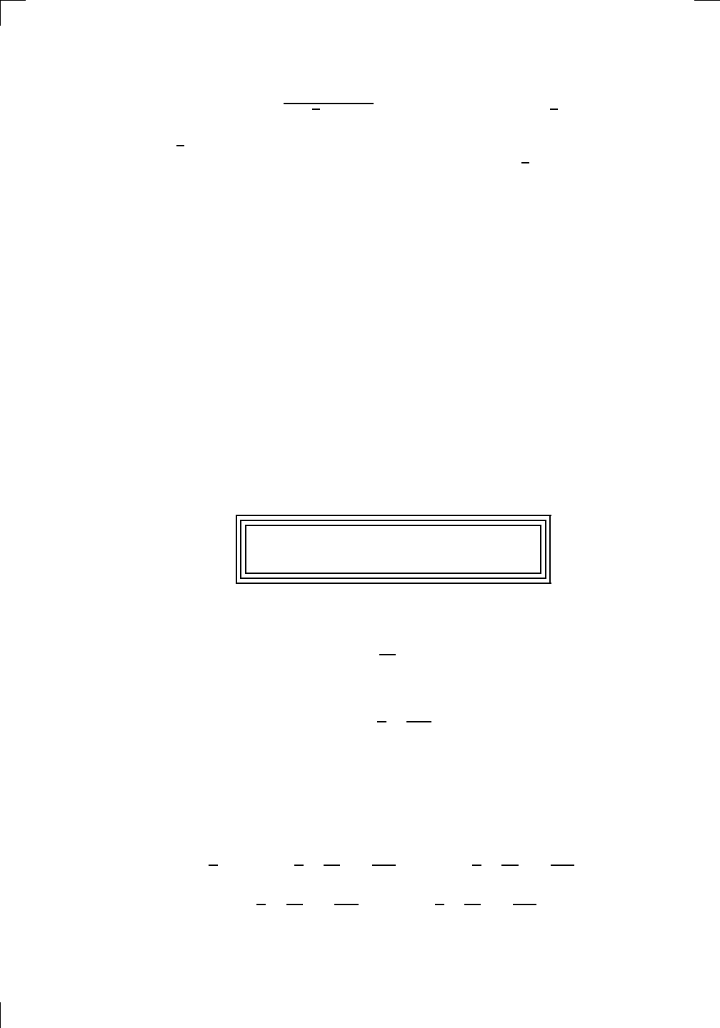
Section 28.4: Solving z
n
= w • 605
So we have R =
q
(−
√
3)
2
+ (1)
2
= 2, and tan(ϕ) = −1/
√
3. Since the
point is in the second quadrant, ϕ must be 5π/6. Great, so we know that
−
√
3 + i = 2e
i(5π/6)
in polar form.
Now let’s turn our attention to the equation z
5
= −
√
3 + i and convert
the whole thing to polar form. On the left, we replace z by re
iθ
to get
z
5
= (re
iθ
)
5
= r
5
e
i(5θ)
, whereas we’ve just seen that the right-hand side is
2e
i(5π/6)
. So our equation becomes
r
5
e
i(5θ)
= 2e
i(5π/6)
.
If you take the modulus of both sides, you get r
5
= 2 (because the modulus
of e
iA
is always 1 if A is real). Then we can cancel out r
5
and 2, since they
are equal, to get e
i(5θ)
= e
i(5π/6)
. We have dissected the above equation into
two separate equations:
r
5
= 2 and e
i(5θ)
= e
i(5π/6)
.
The first is easy to solve: just take the 5th root to get r = 2
1/5
, which is
legit since r is a nonnegative real number. As for the second equation, you
may be tempted to say 5θ = 5π/6, but it’s not that simple. Remember, e
iθ
is 2π-periodic in the variable θ! You can express this fact via the following
important principle, which I want you to remember better than you’ve ever
remembered anything before:
If e
iA
= e
iB
for real numbers A and B, then
A = B + 2πk, where k is an integer.
This principle saves the day. Since e
i(5θ)
= e
i(5π/6)
, we use the principle to
see that
5θ =
5π
6
+ 2πk,
where k is an integer. Dividing by 5, we have
θ =
π
6
+
2πk
5
.
So it looks as if there are infinitely many values of θ, and therefore infinitely
many values of z that solve our equation. Appearances can be deceptive,
however! You see, since n = 5, you only need to use the first five values for
k, namely, k = 0, 1, 2, 3, 4. We’ll see why in just a moment; for now, we can
calculate that as k goes from 0 through 4 inclusive, the values of θ are
π
6
,
π
6
+
2π
5
=
17π
30
,
π
6
+
4π
5
=
29π
30
,
π
6
+
6π
5
=
41π
30
,
π
6
+
8π
5
=
53π
30
,