Banner A. The Calculus Lifesaver: All the Tools You Need to Excel at Calculus
Подождите немного. Документ загружается.


C h a p t e r 29
Volumes, Arc Lengths, and Surface Areas
We have used definite integrals to find areas. Now we’re going to use them to
find volumes, lengths of curves, and surface areas. For volumes and surface
areas, we’ll pay special attention to solids which are formed by revolving a
region in the plane about some axis which lies in the plane; such solids are
called solids of revolution. In the case of volumes, we’ll also look at some more
general solids. Here, then, is the game plan for this chapter:
• finding volumes of solids of revolution using the disc and shell methods;
• finding volumes of more general solids;
• finding arc lengths of smooth curves and speeds of parametric particles;
and
• finding surface areas of solids of revolution.
29.1 Volumes of Solids of Revolution
We’ll start with finding volumes of solids of revolution. The idea is that there
is some region in the plane, and some axis also in the plane, and a solid is
formed by revolving the region about the axis. For our purposes, the axis
will always be parallel to the x-axis or the y-axis. (It is possible to deal
with diagonal axes, but it’s a real pain unless you use techniques from linear
algebra.)
Before we put on our 3D glasses, however, let’s remind ourselves how
definite integrals work. We originally looked at this in Chapter 16, but here’s
a quick review of some of the main ideas. Let’s work in the context of finding
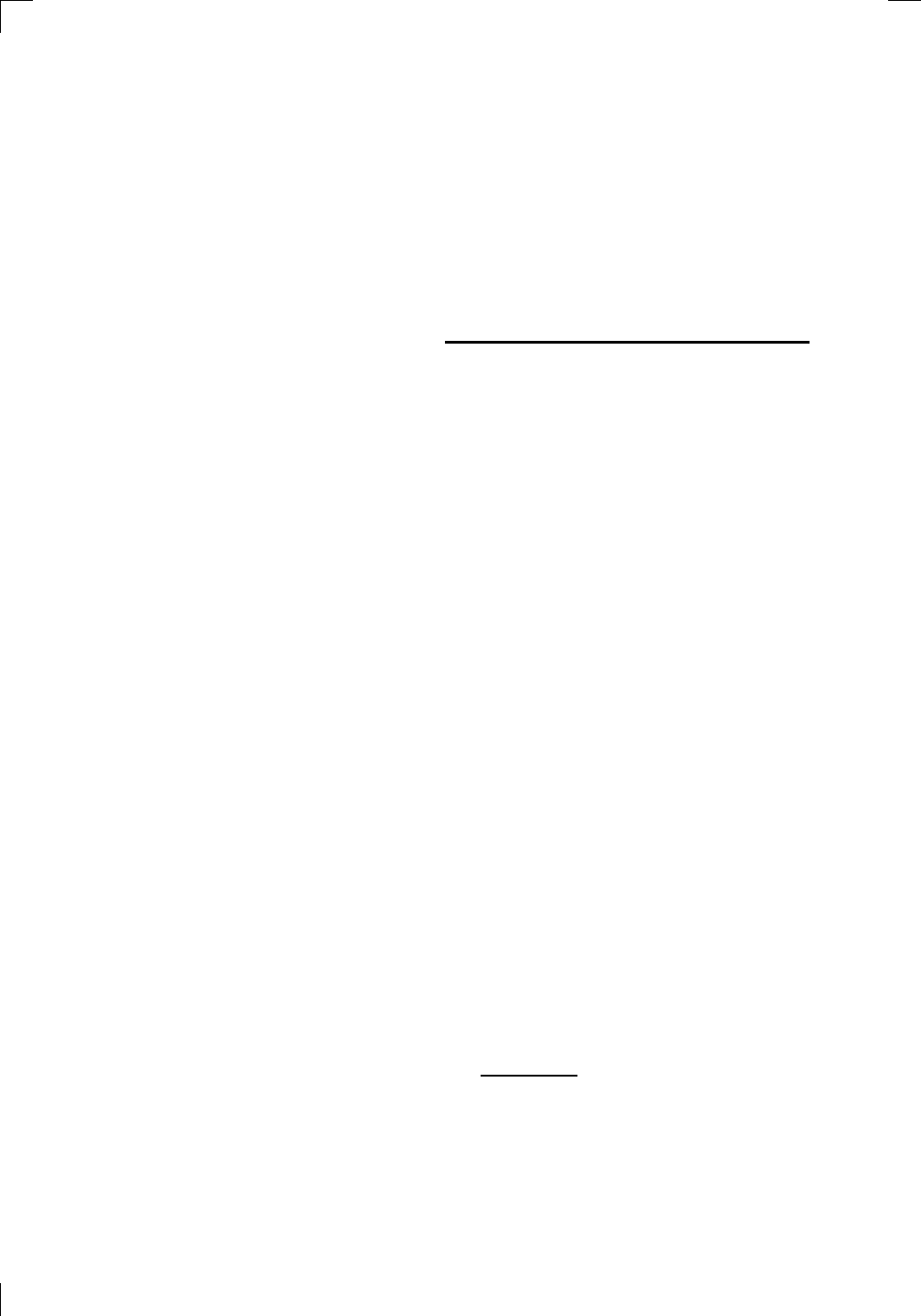
the area of the region below the curve
y =
p
1 − (x − 3)
2
and above the x-axis. What does this look like? Well, if we square the
equation and rearrange, we get (x −3)
2
+ y
2
= 1; the graph of this relation is
the circle of radius 1 unit centered at (3, 0), so our function is the top half of
the circle:
618 • Volumes, Arc Lengths, and Surface Areas
.
PSfrag
replacements
(
a, b)
[
a, b]
(
a, b]
[
a, b)
(
a, ∞)
[
a, ∞)
(
−∞, b)
(
−∞, b]
(
−∞, ∞)
{
x : a < x < b}
{
x : a ≤ x ≤ b}
{
x : a < x ≤ b}
{
x : a ≤ x < b}
{
x : x ≥ a}
{
x : x > a}
{
x : x ≤ b}
{
x : x < b}
R
a
b
shado
w
0
1
4
−
2
3
−
3
g(
x) = x
2
f(
x) = x
3
g(
x) = x
2
f(
x) = x
3
mirror
(y = x)
f
−
1
(x) =
3
√
x
y = h
(x)
y = h
−
1
(x)
y =
(x − 1)
2
−
1
x
Same
height
−
x
Same
length,
opp
osite signs
y = −
2x
−
2
1
y =
1
2
x − 1
2
−
1
y =
2
x
y =
10
x
y =
2
−x
y =
log
2
(x)
4
3
units
mirror
(x-axis)
y = |
x|
y = |
log
2
(x)|
θ radians
θ units
30
◦
=
π
6
45
◦
=
π
4
60
◦
=
π
3
120
◦
=
2
π
3
135
◦
=
3
π
4
150
◦
=
5
π
6
90
◦
=
π
2
180
◦
= π
210
◦
=
7
π
6
225
◦
=
5
π
4
240
◦
=
4
π
3
270
◦
=
3
π
2
300
◦
=
5
π
3
315
◦
=
7
π
4
330
◦
=
11
π
6
0
◦
=
0 radians
θ
hyp
otenuse
opp
osite
adjacen
t
0
(≡ 2π)
π
2
π
3
π
2
I
I
I
I
II
IV
θ
(
x, y)
x
y
r
7
π
6
reference
angle
reference
angle =
π
6
sin
+
sin −
cos
+
cos −
tan
+
tan −
A
S
T
C
7
π
4
9
π
13
5
π
6
(this
angle is
5π
6
clo
ckwise)
1
2
1
2
3
4
5
6
0
−
1
−
2
−
3
−
4
−
5
−
6
−
3π
−
5
π
2
−
2π
−
3
π
2
−
π
−
π
2
3
π
3
π
5
π
2
2
π
3
π
2
π
π
2
y =
sin(x)
1
0
−
1
−
3π
−
5
π
2
−
2π
−
3
π
2
−
π
−
π
2
3
π
5
π
2
2
π
2
π
3
π
2
π
π
2
y =
sin(x)
y =
cos(x)
−
π
2
π
2
y =
tan(x), −
π
2
<
x <
π
2
0
−
π
2
π
2
y =
tan(x)
−
2π
−
3π
−
5
π
2
−
3
π
2
−
π
−
π
2
π
2
3
π
3
π
5
π
2
2
π
3
π
2
π
y =
sec(x)
y =
csc(x)
y =
cot(x)
y = f (
x)
−
1
1
2
y = g(
x)
3
y = h
(x)
4
5
−
2
f(
x) =
1
x
g(
x) =
1
x
2
etc.
0
1
π
1
2
π
1
3
π
1
4
π
1
5
π
1
6
π
1
7
π
g(
x) = sin
1
x
1
0
−
1
L
10
100
200
y =
π
2
y = −
π
2
y =
tan
−1
(x)
π
2
π
y =
sin(
x)
x
,
x > 3
0
1
−
1
a
L
f(
x) = x sin (1/x)
(0 <
x < 0.3)
h
(x) = x
g(
x) = −x
a
L
lim
x
→a
+
f(x) = L
lim
x
→a
+
f(x) = ∞
lim
x
→a
+
f(x) = −∞
lim
x
→a
+
f(x) DNE
lim
x
→a
−
f(x) = L
lim
x
→a
−
f(x) = ∞
lim
x
→a
−
f(x) = −∞
lim
x
→a
−
f(x) DNE
M
}
lim
x
→a
−
f(x) = M
lim
x
→a
f(x) = L
lim
x
→a
f(x) DNE
lim
x
→∞
f(x) = L
lim
x
→∞
f(x) = ∞
lim
x
→∞
f(x) = −∞
lim
x
→∞
f(x) DNE
lim
x
→−∞
f(x) = L
lim
x
→−∞
f(x) = ∞
lim
x
→−∞
f(x) = −∞
lim
x
→−∞
f(x) DNE
lim
x →a
+
f(
x) = ∞
lim
x →a
+
f(
x) = −∞
lim
x →a
−
f(
x) = ∞
lim
x →a
−
f(
x) = −∞
lim
x →a
f(
x) = ∞
lim
x →a
f(
x) = −∞
lim
x →a
f(
x) DNE
y = f (
x)
a
y =
|
x|
x
1
−
1
y =
|
x + 2|
x +
2
1
−
1
−
2
1
2
3
4
a
a
b
y = x sin
1
x
y = x
y = −
x
a
b
c
d
C
a
b
c
d
−
1
0
1
2
3
time
y
t
u
(
t, f(t))
(
u, f(u))
time
y
t
u
y
x
(
x, f(x))
y = |
x|
(
z, f(z))
z
y = f (
x)
a
tangen
t at x = a
b
tangen
t at x = b
c
tangen
t at x = c
y = x
2
tangen
t
at x = −
1
u
v
uv
u +
∆u
v +
∆v
(
u + ∆u)(v + ∆v)
∆
u
∆
v
u
∆v
v∆
u
∆
u∆v
y = f (
x)
1
2
−
2
y = |
x
2
− 4|
y = x
2
− 4
y = −
2x + 5
y = g(
x)
1
2
3
4
5
6
7
8
9
0
−
1
−
2
−
3
−
4
−
5
−
6
y = f (
x)
3
−
3
3
−
3
0
−
1
2
easy
hard
flat
y = f
0
(
x)
3
−
3
0
−
1
2
1
−
1
y =
sin(x)
y = x
x
A
B
O
1
C
D
sin(
x)
tan(
x)
y =
sin
(x)
x
π
2
π
1
−
1
x =
0
a =
0
x
> 0
a
> 0
x
< 0
a
< 0
rest
position
+
−
y = x
2
sin
1
x
N
A
B
H
a
b
c
O
H
A
B
C
D
h
r
R
θ
1000
2000
α
β
p
h
y = g(
x) = log
b
(x)
y = f(
x) = b
x
y = e
x
5
10
1
2
3
4
0
−
1
−
2
−
3
−
4
y =
ln(x)
y =
cosh(x)
y =
sinh(x)
y =
tanh(x)
y =
sech(x)
y =
csch(x)
y =
coth(x)
1
−
1
y = f (
x)
original
function
in
verse function
slop
e = 0 at (x, y)
slop
e is infinite at (y, x)
−
108
2
5
1
2
1
2
3
4
5
6
0
−
1
−
2
−
3
−
4
−
5
−
6
−
3π
−
5
π
2
−
2π
−
3
π
2
−
π
−
π
2
3
π
3
π
5
π
2
2
π
3
π
2
π
π
2
y =
sin(x)
1
0
−
1
−
3π
−
5
π
2
−
2π
−
3
π
2
−
π
−
π
2
3
π
5
π
2
2
π
2
π
3
π
2
π
π
2
y =
sin(x)
y =
sin(x), −
π
2
≤ x ≤
π
2
−
2
−
1
0
2
π
2
−
π
2
y =
sin
−1
(x)
y =
cos(x)
π
π
2
y =
cos
−1
(x)
−
π
2
1
x
α
β
y =
tan(x)
y =
tan(x)
1
y =
tan
−1
(x)
y =
sec(x)
y =
sec
−1
(x)
y =
csc
−1
(x)
y =
cot
−1
(x)
1
y =
cosh
−1
(x)
y =
sinh
−1
(x)
y =
tanh
−1
(x)
y =
sech
−1
(x)
y =
csch
−1
(x)
y =
coth
−1
(x)
(0
, 3)
(2
, −1)
(5
, 2)
(7
, 0)
(
−1, 44)
(0
, 1)
(1
, −12)
(2
, 305)
y =
1
2
(2
, 3)
y = f (
x)
y = g(
x)
a
b
c
a
b
c
s
c
0
c
1
(
a, f(a))
(
b, f(b))
1
2
1
2
3
4
5
6
0
−
1
−
2
−
3
−
4
−
5
−
6
−
3π
−
5
π
2
−
2π
−
3
π
2
−
π
−
π
2
3
π
3
π
5
π
2
2
π
3
π
2
π
π
2
y =
sin(x)
1
0
−
1
−
3π
−
5
π
2
−
2π
−
3
π
2
−
π
−
π
2
3
π
5
π
2
2
π
2
π
3
π
2
π
π
2
c
OR
Lo
cal maximum
Lo
cal minimum
Horizon
tal point of inflection
1
e
y = f
0
(
x)
y = f(
x) = x ln(x)
−
1
e
?
y = f(
x) = x
3
y = g(
x) = x
4
x
f(
x)
−
3
−
2
−
1
0
1
2
1
2
3
4
+
−
?
1
5
6
3
f
0
(
x)
2 −
1
2
√
6
2
+
1
2
√
6
f
00
(
x)
7
8
g
00
(
x)
f
00
(
x)
0
y =
(
x − 3)(x − 1)
2
x
3
(
x + 2)
y = x ln
(x)
1
e
−
1
e
5
−
108
2
α
β
2 −
1
2
√
6
2
+
1
2
√
6
y = x
2
(
x − 5)
3
−
e
−
1/2
√
3
e
−
1/2
√
3
−
e
−3/2
e
−
3/2
−
1
√
3
1
√
3
−
1
1
y = xe
−
3x
2
/2
y =
x
3
− 6
x
2
+ 13x − 8
x
28
2
600
500
400
300
200
100
0
−
100
−
200
−
300
−
400
−
500
−
600
0
10
−
10
5
−
5
20
−
20
15
−
15
0
4
5
6
x
P
0
(
x)
+
−
−
existing
fence
new
fence
enclosure
A
h
b
H
99
100
101
h
dA/dh
r
h
1
2
7
shallo
w
deep
LAND
SEA
N
y
z
s
t
3
11
9
L
(11)
√
11
y = L
(x)
y = f (
x)
11
y = L
(x)
y = f (
x)
F
P
a
a +
∆x
f(
a + ∆x)
L
(a + ∆x)
f(
a)
error
d
f
∆
x
a
b
y = f (
x)
true
zero
starting
approximation
b
etter approximation
v
t
3
5
50
40
60
4
20
30
25
t
1
t
2
t
3
t
4
t
n
−2
t
n
−1
t
0
= a
t
n
= b
v
1
v
2
v
3
v
4
v
n
−1
v
n
−
30
6
30
|
v|
a
b
p
q
c
v(
c)
v(
c
1
)
v(
c
2
)
v(
c
3
)
v(
c
4
)
v(
c
5
)
v(
c
6
)
t
1
t
2
t
3
t
4
t
5
c
1
c
2
c
3
c
4
c
5
c
6
t
0
=
a
t
6
=
b
t
16
=
b
t
10
=
b
a
b
x
y
y = f (
x)
1
2
y = x
5
0
−
2
y =
1
a
b
y =
sin(x)
π
−
π
0
−
1
−
2
0
2
4
y = x
2
0
1
2
3
4
2
n
4
n
6
n
2(
n−2)
n
2(
n−1)
n
2
n
n
=
2
width
of each interval =
2
n
−
2
1
3
0
I
I
I
I
II
IV
4
y
dx
y = −
x
2
− 2x + 3
3
−
5
y = |−
x
2
− 2x + 3|
I
I
I
I
Ia
5
3
0
1
2
a
b
y = f (
x)
y = g(
x)
y = x
2
a
b
5
3
0
1
2
y =
√
x
2
√
2
2
2
dy
x
2
a
b
y = f (
x)
y = g(
x)
M
m
1
2
−
1
−
2
0
y = e
−
x
2
1
2
e
−
1/4
f
a
v
y = f
a
v
c
A
M
0
1
2
a
b
x
t
y = f(
t)
F (
x )
y = f(
t)
F (
x + h )
x + h
F (
x + h) − F (x)
f(
x)
1
2
y =
sin(x)
π
−
π
−
1
−
2
y =
1
x
y = x
2
1
2
1
−
1
y =
ln|x|
θ
a
x
a
x
p
a
2
− x
2
3
x
p
9 − x
2
p
x
2
+ a
2
x
a
p
x
2
+ 15
x
√
15
x
p
x
2
− a
2
a
x
p
x
2
− 4
2
x
−
p
x
2
− a
2
a
x
−
p
x
2
− 4
2
y = f (
x)
a
b
a + ε
ε
Z
b
a
+ε
f(x) dx
small
ev
en smaller
y = g(
x)
infinite
area
finite
area
1
y =
1
x
y =
1
x
p
, p
< 1 (typical)
y =
1
x
p
, p
> 1 (typical)
a
1
a
2
a
3
a
4
a
5
a
6
a
7
a
8
1
2
3
4
5
6
7
8
n
a
n
x
y
y = f (
x)
(
a, f(a))
a
−
1
0
1
a
6
1
2
7
1
2
7
?
−
2
−
1
−
2
t =
0
t = π
/6
t = π
/4
t = π
/3
t = π
/2
3
0
t = −
2
t = −
3/2
t = ±
1
t = −
1/2
t =
0
t =
1/2
t =
3/2
t =
2
12
−
12
θ
r
P
θ
r
P
11
π
6
2
(
−1, −1)
wrong
point
π
4
5
π
4
√
2
(0
, 1)
(0
, −3)
(
−2, 0)
π
2
3
π
2
π
r =
3 sin(θ)
3
π
2
θ
2
π
1
0
−
1
−
2
−
3
0
3
2
−
3
2
0
r =
1 + 2 cos(θ)
2
π
3
4
π
3
0
π
0
pi
−
3
2
3
π
2
1
2
3
0
−
1
−
2
−
3
0 ≤ θ ≤
2
π
3
0 ≤ θ ≤ π
0 ≤ θ ≤ 2
π
r =
1 + cos(θ)
r =
1 +
3
4
cos(
θ)
−
1
4
r =
sin(2θ)
r =
sin(3θ)
r =
1
π
θ
0 ≤ θ ≤ 4
π
r =
2
1
+ sin(θ)
−
π
4
≤ θ ≤
5
π
4
0 ≤ θ ≤ 2
π
0 ≤ θ ≤ π
−
4
−
5
4
5
f(
θ)
f(
θ + dθ)
θ
dθ
θ + dθ
approximating region
exact region
0 ≤ θ ≤ 2π
r = |1 + 2 cos(θ)|
2i
2 − 3i
−1
θ = 0
θ =
π
4
θ =
π
2
θ =
2π
3
θ = π
θ =
13π
12
θ =
3π
2
θ =
7π
4
1 = e
0
e
i
π
4
i = e
i
π
2
e
i
2π
3
−1 = e
iπ
e
i
13π
12
−i = e
i
3π
2
e
i
7π
4
i
−i
1
θ
1 − i
2i
−2i
2
−2
6i
−6i
6
−6
−
√
3
R
ϕ
2
1/5
θ =
π
6
θ =
17π
30
θ =
29π
30
θ =
41π
30
θ =
53π
30
z
0
z
1
z
2
z
3
z
4
−
√
3
2
√
3
2
1
2
i
−i
19π
6
−i
7π
6
i
5π
6
i
17π
6
i
29π
6
ln(2)
−
7π
4
−
3π
4
π
4
5π
4
9π
4
3
2
i
0
1 2
3 4
dx
y
x
y =
p
1 − (x − 3)
2
By the definition of the definite integral, we know that the shaded area (in
square units) is
Z
4
2
p
1 − (x − 3)
2
dx
which can also be written as
R
4
2
y dx.
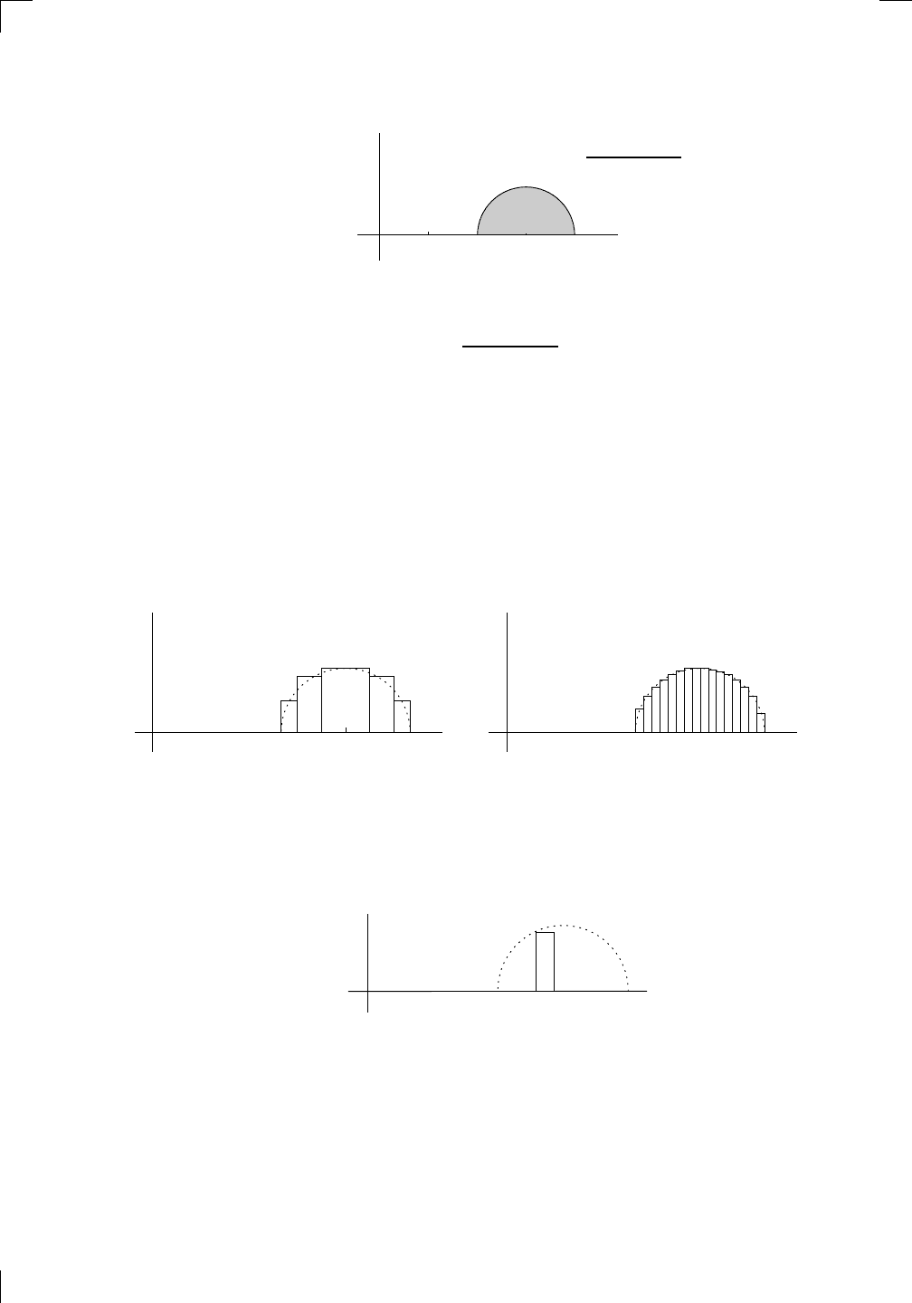
On the other hand, to find the area of this semicircle using a Riemann
sum, we have to chop the base on the x-axis into little segments, then build
the segments up into strips. The strips don’t have to have the same width,
and the only thing you need to make sure of is that the top of each strip cuts
the curve somewhere (or touches the curve at one of its corners). The total
area of the strips can easily be worked out, since it is just the sum of areas of
rectangles. This area is an approximation for the actual area of the semicircle;
the thinner the strips, the better the approximation, as you can see:
PSfrag
replacements
(
a, b)
[
a, b]
(
a, b]
[
a, b)
(
a, ∞)
[
a, ∞)
(
−∞, b)
(
−∞, b]
(
−∞, ∞)
{
x : a < x < b}
{
x : a ≤ x ≤ b}
{
x : a < x ≤ b}
{
x : a ≤ x < b}
{
x : x ≥ a}
{
x : x > a}
{
x : x ≤ b}
{
x : x < b}
R
a
b
shado
w
0
1
4
−
2
3
−
3
g(
x) = x
2
f(
x) = x
3
g(
x) = x
2
f(
x) = x
3
mirror
(y = x)
f
−
1
(x) =
3
√
x
y = h
(x)
y = h
−
1
(x)
y =
(x − 1)
2
−
1
x
Same
height
−
x
Same
length,
opp
osite signs
y = −
2x
−
2
1
y =
1
2
x − 1
2
−
1
y =
2
x
y =
10
x
y =
2
−x
y =
log
2
(x)
4
3
units
mirror
(x-axis)
y = |
x|
y = |
log
2
(x)|
θ radians
θ units
30
◦
=
π
6
45
◦
=
π
4
60
◦
=
π
3
120
◦
=
2
π
3
135
◦
=
3
π
4
150
◦
=
5
π
6
90
◦
=
π
2
180
◦
= π
210
◦
=
7
π
6
225
◦
=
5
π
4
240
◦
=
4
π
3
270
◦
=
3
π
2
300
◦
=
5
π
3
315
◦
=
7
π
4
330
◦
=
11
π
6
0
◦
=
0 radians
θ
h
yp
otenuse
opp
osite
adjacen
t
0
(≡ 2π)
π
2
π
3
π
2
I
I
I
I
II
IV
θ
(
x, y)
x
y
r
7
π
6
reference
angle
reference
angle =
π
6
sin
+
sin −
cos
+
cos −
tan
+
tan −
A
S
T
C
7
π
4
9
π
13
5
π
6
(this
angle is
5π
6
clo
ckwise)
1
2
1
2
3
4
5
6
0
−
1
−
2
−
3
−
4
−
5
−
6
−
3π
−
5
π
2
−
2π
−
3
π
2
−
π
−
π
2
3
π
3
π
5
π
2
2
π
3
π
2
π
π
2
y =
sin(x)
1
0
−
1
−
3π
−
5
π
2
−
2π
−
3
π
2
−
π
−
π
2
3
π
5
π
2
2
π
2
π
3
π
2
π
π
2
y =
sin(x)
y =
cos(x)
−
π
2
π
2
y =
tan(x), −
π
2
<
x <
π
2
0
−
π
2
π
2
y =
tan(x)
−
2π
−
3π
−
5
π
2
−
3
π
2
−
π
−
π
2
π
2
3
π
3
π
5
π
2
2
π
3
π
2
π
y =
sec(x)
y =
csc(x)
y =
cot(x)
y = f(
x)
−
1
1
2
y = g(
x)
3
y = h
(x)
4
5
−
2
f(
x) =
1
x
g(
x) =
1
x
2
etc.
0
1
π
1
2
π
1
3
π
1
4
π
1
5
π
1
6
π
1
7
π
g(
x) = sin
1
x
1
0
−
1
L
10
100
200
y =
π
2
y = −
π
2
y =
tan
−1
(x)
π
2
π
y =
sin(
x)
x
,
x > 3
0
1
−
1
a
L
f(
x) = x sin (1/x)
(0 <
x < 0.3)
h
(x) = x
g(
x) = −x
a
L
lim
x
→a
+
f(x) = L
lim
x
→a
+
f(x) = ∞
lim
x
→a
+
f(x) = −∞
lim
x
→a
+
f(x) DNE
lim
x
→a
−
f(x) = L
lim
x
→a
−
f(x) = ∞
lim
x
→a
−
f(x) = −∞
lim
x
→a
−
f(x) DNE
M
}
lim
x
→a
−
f(x) = M
lim
x
→a
f(x) = L
lim
x
→a
f(x) DNE
lim
x
→∞
f(x) = L
lim
x
→∞
f(x) = ∞
lim
x
→∞
f(x) = −∞
lim
x
→∞
f(x) DNE
lim
x
→−∞
f(x) = L
lim
x
→−∞
f(x) = ∞
lim
x
→−∞
f(x) = −∞
lim
x
→−∞
f(x) DNE
lim
x →a
+
f(
x) = ∞
lim
x →a
+
f(
x) = −∞
lim
x →a
−
f(
x) = ∞
lim
x →a
−
f(
x) = −∞
lim
x →a
f(
x) = ∞
lim
x →a
f(
x) = −∞
lim
x →a
f(
x) DNE
y = f(
x)
a
y =
|
x|
x
1
−
1
y =
|
x + 2|
x +
2
1
−
1
−
2
1
2
3
4
a
a
b
y = x sin
1
x
y = x
y = −
x
a
b
c
d
C
a
b
c
d
−
1
0
1
2
3
time
y
t
u
(
t, f(t))
(
u, f(u))
time
y
t
u
y
x
(
x, f(x))
y = |
x|
(
z, f(z))
z
y = f(
x)
a
tangen
t at x = a
b
tangen
t at x = b
c
tangen
t at x = c
y = x
2
tangen
t
at x = −
1
u
v
uv
u +
∆u
v +
∆v
(
u + ∆u)(v + ∆v)
∆
u
∆
v
u
∆v
v∆
u
∆
u∆v
y = f(
x)
1
2
−
2
y = |
x
2
− 4|
y = x
2
− 4
y = −
2x + 5
y = g(
x)
1
2
3
4
5
6
7
8
9
0
−
1
−
2
−
3
−
4
−
5
−
6
y = f(
x)
3
−
3
3
−
3
0
−
1
2
easy
hard
flat
y = f
0
(
x)
3
−
3
0
−
1
2
1
−
1
y =
sin(x)
y = x
x
A
B
O
1
C
D
sin
(x)
tan
(x)
y =
sin
(x)
x
π
2
π
1
−
1
x =
0
a =
0
x
> 0
a
> 0
x
< 0
a
< 0
rest
position
+
−
y = x
2
sin
1
x
N
A
B
H
a
b
c
O
H
A
B
C
D
h
r
R
θ
1000
2000
α
β
p
h
y = g(
x) = log
b
(x)
y = f(
x) = b
x
y = e
x
5
10
1
2
3
4
0
−
1
−
2
−
3
−
4
y =
ln(x)
y =
cosh(x)
y =
sinh(x)
y =
tanh(x)
y =
sech(x)
y =
csch(x)
y =
coth(x)
1
−
1
y = f(
x)
original
function
in
verse function
slop
e = 0 at (x, y)
slop
e is infinite at (y, x)
−
108
2
5
1
2
1
2
3
4
5
6
0
−
1
−
2
−
3
−
4
−
5
−
6
−
3π
−
5
π
2
−
2π
−
3
π
2
−
π
−
π
2
3
π
3
π
5
π
2
2
π
3
π
2
π
π
2
y =
sin(x)
1
0
−
1
−
3π
−
5
π
2
−
2π
−
3
π
2
−
π
−
π
2
3
π
5
π
2
2
π
2
π
3
π
2
π
π
2
y =
sin(x)
y =
sin(x), −
π
2
≤ x ≤
π
2
−
2
−
1
0
2
π
2
−
π
2
y =
sin
−1
(x)
y =
cos(x)
π
π
2
y =
cos
−1
(x)
−
π
2
1
x
α
β
y =
tan(x)
y =
tan(x)
1
y =
tan
−1
(x)
y =
sec(x)
y =
sec
−1
(x)
y =
csc
−1
(x)
y =
cot
−1
(x)
1
y =
cosh
−1
(x)
y =
sinh
−1
(x)
y =
tanh
−1
(x)
y =
sech
−1
(x)
y =
csch
−1
(x)
y =
coth
−1
(x)
(0
, 3)
(2
, −1)
(5
, 2)
(7
, 0)
(
−1, 44)
(0
, 1)
(1
, −12)
(2
, 305)
y =
1
2
(2
, 3)
y = f(
x)
y = g(
x)
a
b
c
a
b
c
s
c
0
c
1
(
a, f(a))
(
b, f(b))
1
2
1
2
3
4
5
6
0
−
1
−
2
−
3
−
4
−
5
−
6
−
3π
−
5
π
2
−
2π
−
3
π
2
−
π
−
π
2
3
π
3
π
5
π
2
2
π
3
π
2
π
π
2
y =
sin(x)
1
0
−
1
−
3π
−
5
π
2
−
2π
−
3
π
2
−
π
−
π
2
3
π
5
π
2
2
π
2
π
3
π
2
π
π
2
c
OR
Lo
cal maximum
Lo
cal minimum
Horizon
tal point of inflection
1
e
y = f
0
(
x)
y = f(
x) = x ln(x)
−
1
e
?
y = f (
x) = x
3
y = g(
x) = x
4
x
f(
x)
−
3
−
2
−
1
0
1
2
1
2
3
4
+
−
?
1
5
6
3
f
0
(
x)
2 −
1
2
√
6
2
+
1
2
√
6
f
00
(
x)
7
8
g
00
(
x)
f
00
(
x)
0
y =
(
x − 3)(x − 1)
2
x
3
(
x + 2)
y = x ln(
x)
1
e
−
1
e
5
−
108
2
α
β
2 −
1
2
√
6
2
+
1
2
√
6
y = x
2
(
x − 5)
3
−
e
−
1/2
√
3
e
−
1/2
√
3
−
e
−3/2
e
−
3/2
−
1
√
3
1
√
3
−
1
1
y = xe
−
3x
2
/2
y =
x
3
− 6
x
2
+ 13x − 8
x
28
2
600
500
400
300
200
100
0
−
100
−
200
−
300
−
400
−
500
−
600
0
10
−
10
5
−
5
20
−
20
15
−
15
0
4
5
6
x
P
0
(
x)
+
−
−
existing
fence
new
fence
enclosure
A
h
b
H
99
100
101
h
dA/dh
r
h
1
2
7
shallo
w
deep
LAND
SEA
N
y
z
s
t
3
11
9
L
(11)
√
11
y = L
(x)
y = f(
x)
11
y = L
(x)
y = f(
x)
F
P
a
a +
∆x
f(
a + ∆x)
L
(a + ∆x)
f(
a)
error
d
f
∆
x
a
b
y = f(
x)
true
zero
starting
approximation
b
etter approximation
v
t
3
5
50
40
60
4
20
30
25
t
1
t
2
t
3
t
4
t
n
−2
t
n
−1
t
0
= a
t
n
= b
v
1
v
2
v
3
v
4
v
n
−1
v
n
−
30
6
30
|
v|
a
b
p
q
c
v(
c)
v(
c
1
)
v(
c
2
)
v(
c
3
)
v(
c
4
)
v(
c
5
)
v(
c
6
)
t
1
t
2
t
3
t
4
t
5
c
1
c
2
c
3
c
4
c
5
c
6
t
0
=
a
t
6
=
b
t
16
=
b
t
10
=
b
a
b
x
y
y = f(
x)
1
2
y = x
5
0
−
2
y =
1
a
b
y =
sin(x)
π
−
π
0
−
1
−
2
0
2
4
y = x
2
0
1
2
3
4
2
n
4
n
6
n
2(
n−2)
n
2(
n−1)
n
2
n
n
=
2
width
of each interval =
2
n
−
2
1
3
0
I
I
I
I
II
IV
4
y
dx
y = −
x
2
− 2x + 3
3
−
5
y = |−
x
2
− 2x + 3|
I
I
I
I
Ia
5
3
0
1
2
a
b
y = f (
x)
y = g(
x)
y = x
2
a
b
5
3
0
1
2
y =
√
x
2
√
2
2
2
dy
x
2
a
b
y = f(
x)
y = g(
x)
M
m
1
2
−
1
−
2
0
y = e
−
x
2
1
2
e
−
1/4
f
a
v
y = f
a
v
c
A
M
0
1
2
a
b
x
t
y = f (
t)
F (
x )
y = f (
t)
F (
x + h)
x + h
F (
x + h) − F (x)
f(
x)
1
2
y =
sin(x)
π
−
π
−
1
−
2
y =
1
x
y = x
2
1
2
1
−
1
y =
ln|x|
θ
a
x
a
x
p
a
2
− x
2
3
x
p
9 − x
2
p
x
2
+ a
2
x
a
p
x
2
+ 15
x
√
15
x
p
x
2
− a
2
a
x
p
x
2
− 4
2
x
−
p
x
2
− a
2
a
x
−
p
x
2
− 4
2
y = f(
x)
a
b
a + ε
ε
Z
b
a
+ε
f(x) dx
small
ev
en smaller
y = g(
x)
infinite
area
finite
area
1
y =
1
x
y =
1
x
p
, p
< 1 (typical)
y =
1
x
p
, p
> 1 (typical)
a
1
a
2
a
3
a
4
a
5
a
6
a
7
a
8
1
2
3
4
5
6
7
8
n
a
n
x
y
y = f(
x)
(
a, f(a))
a
−
1
0
1
a
6
1
2
7
1
2
7
?
−
2
−
1
−
2
t =
0
t = π
/6
t = π
/4
t = π
/3
t = π
/2
3
0
t = −
2
t = −
3/2
t = ±
1
t = −
1/2
t =
0
t =
1/2
t =
3/2
t =
2
12
−
12
θ
r
P
θ
r
P
11
π
6
2
(
−1, −1)
wrong
point
π
4
5
π
4
√
2
(0
, 1)
(0
, −3)
(
−2, 0)
π
2
3
π
2
π
r =
3 sin(θ)
3
π
2
θ
2
π
1
0
−
1
−
2
−
3
0
3
2
−
3
2
0
r =
1 + 2 cos(θ)
2
π
3
4
π
3
0
π
0
pi
−
3
2
3
π
2
1
2
3
0
−
1
−
2
−
3
0 ≤ θ ≤
2
π
3
0 ≤ θ ≤ π
0 ≤ θ ≤ 2
π
r =
1 + cos(θ)
r =
1 +
3
4
cos(θ)
−
1
4
r = sin(2θ)
r = sin(3θ)
r =
1
π
θ
0 ≤ θ ≤ 4π
r =
2
1 + sin(θ)
−
π
4
≤ θ ≤
5π
4
0 ≤ θ ≤ 2π
0 ≤ θ ≤ π
−4
−5
4
5
f(θ)
f(θ + dθ)
θ
dθ
θ + dθ
approximating region
exact region
0 ≤ θ ≤ 2π
r = |1 + 2 cos(θ)|
2i
2 − 3i
−1
θ = 0
θ =
π
4
θ =
π
2
θ =
2π
3
θ = π
θ =
13π
12
θ =
3π
2
θ =
7π
4
1 = e
0
e
i
π
4
i = e
i
π
2
e
i
2π
3
−1 = e
iπ
e
i
13π
12
−i = e
i
3π
2
e
i
7π
4
i
−i
1
θ
1 − i
2i
−2i
2
−2
6i
−6i
6
−6
−
√
3
R
ϕ
2
1/5
θ =
π
6
θ =
17π
30
θ =
29π
30
θ =
41π
30
θ =
53π
30
z
0
z
1
z
2
z
3
z
4
−
√
3
2
√
3
2
1
2
i
−i
19π
6
−i
7π
6
i
5π
6
i
17π
6
i
29π
6
ln(2)
−
7π
4
−
3π
4
π
4
5π
4
9π
4
3
2
i
0
1
22
33
44
dx
y
x
y =
p
1 − (x − 3)
2
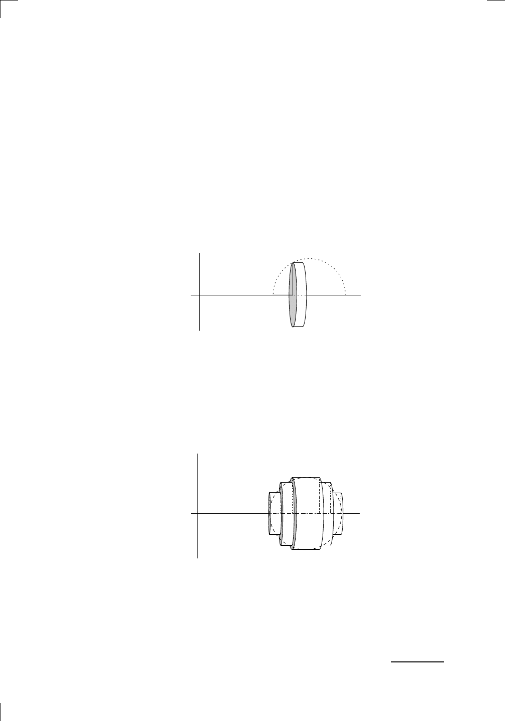
Let’s just check out one generic strip. To make things a little easier, we’ll
assume that the top left-hand corner lies on the curve. As we’ve seen in
Section 16.4 of Chapter 16, it doesn’t matter which strips you choose, as long
as the tops of all the strips pass through the curve. Anyway, here’s what one
strip looks like:
PSfrag
replacements
(
a, b)
[
a, b]
(
a, b]
[
a, b)
(
a, ∞)
[
a, ∞)
(
−∞, b)
(
−∞, b]
(
−∞, ∞)
{
x : a < x < b}
{
x : a ≤ x ≤ b}
{
x : a < x ≤ b}
{
x : a ≤ x < b}
{
x : x ≥ a}
{
x : x > a}
{
x : x ≤ b}
{
x : x < b}
R
a
b
shado
w
0
1
4
−
2
3
−
3
g(
x) = x
2
f(
x) = x
3
g(
x) = x
2
f(
x) = x
3
mirror
(y = x)
f
−
1
(x) =
3
√
x
y = h
(x)
y = h
−
1
(x)
y =
(x − 1)
2
−
1
x
Same
height
−
x
Same
length,
opp
osite signs
y = −
2x
−
2
1
y =
1
2
x − 1
2
−
1
y =
2
x
y =
10
x
y =
2
−x
y =
log
2
(x)
4
3
units
mirror
(x-axis)
y = |
x|
y = |
log
2
(x)|
θ radians
θ units
30
◦
=
π
6
45
◦
=
π
4
60
◦
=
π
3
120
◦
=
2
π
3
135
◦
=
3
π
4
150
◦
=
5
π
6
90
◦
=
π
2
180
◦
= π
210
◦
=
7
π
6
225
◦
=
5
π
4
240
◦
=
4
π
3
270
◦
=
3
π
2
300
◦
=
5
π
3
315
◦
=
7
π
4
330
◦
=
11
π
6
0
◦
=
0 radians
θ
hyp
otenuse
opp
osite
adjacen
t
0
(≡ 2π)
π
2
π
3
π
2
I
I
I
I
II
IV
θ
(
x, y)
x
y
r
7
π
6
reference
angle
reference
angle =
π
6
sin
+
sin −
cos
+
cos −
tan
+
tan −
A
S
T
C
7
π
4
9
π
13
5
π
6
(this
angle is
5π
6
clo
ckwise)
1
2
1
2
3
4
5
6
0
−
1
−
2
−
3
−
4
−
5
−
6
−
3π
−
5
π
2
−
2π
−
3
π
2
−
π
−
π
2
3
π
3
π
5
π
2
2
π
3
π
2
π
π
2
y =
sin(x)
1
0
−
1
−
3π
−
5
π
2
−
2π
−
3
π
2
−
π
−
π
2
3
π
5
π
2
2
π
2
π
3
π
2
π
π
2
y =
sin(x)
y =
cos(x)
−
π
2
π
2
y =
tan(x), −
π
2
<
x <
π
2
0
−
π
2
π
2
y =
tan(x)
−
2π
−
3π
−
5
π
2
−
3
π
2
−
π
−
π
2
π
2
3
π
3
π
5
π
2
2
π
3
π
2
π
y =
sec(x)
y =
csc(x)
y =
cot(x)
y = f(
x)
−
1
1
2
y = g(
x)
3
y = h
(x)
4
5
−
2
f(
x) =
1
x
g(
x) =
1
x
2
etc.
0
1
π
1
2
π
1
3
π
1
4
π
1
5
π
1
6
π
1
7
π
g(
x) = sin
1
x
1
0
−
1
L
10
100
200
y =
π
2
y = −
π
2
y =
tan
−1
(x)
π
2
π
y =
sin(
x)
x
,
x > 3
0
1
−
1
a
L
f(
x) = x sin (1/x)
(0 <
x < 0.3)
h
(x) = x
g(
x) = −x
a
L
lim
x
→a
+
f(x) = L
lim
x
→a
+
f(x) = ∞
lim
x
→a
+
f(x) = −∞
lim
x
→a
+
f(x) DNE
lim
x
→a
−
f(x) = L
lim
x
→a
−
f(x) = ∞
lim
x
→a
−
f(x) = −∞
lim
x
→a
−
f(x) DNE
M
}
lim
x
→a
−
f(x) = M
lim
x
→a
f(x) = L
lim
x
→a
f(x) DNE
lim
x
→∞
f(x) = L
lim
x
→∞
f(x) = ∞
lim
x
→∞
f(x) = −∞
lim
x
→∞
f(x) DNE
lim
x
→−∞
f(x) = L
lim
x
→−∞
f(x) = ∞
lim
x
→−∞
f(x) = −∞
lim
x
→−∞
f(x) DNE
lim
x →a
+
f(
x) = ∞
lim
x →a
+
f(
x) = −∞
lim
x →a
−
f(
x) = ∞
lim
x →a
−
f(
x) = −∞
lim
x →a
f(
x) = ∞
lim
x →a
f(
x) = −∞
lim
x →a
f(
x) DNE
y = f(
x)
a
y =
|
x|
x
1
−
1
y =
|
x + 2|
x +
2
1
−
1
−
2
1
2
3
4
a
a
b
y = x sin
1
x
y = x
y = −
x
a
b
c
d
C
a
b
c
d
−
1
0
1
2
3
time
y
t
u
(
t, f(t))
(
u, f(u))
time
y
t
u
y
x
(
x, f(x))
y = |
x|
(
z, f(z))
z
y = f(
x)
a
tangen
t at x = a
b
tangen
t at x = b
c
tangen
t at x = c
y = x
2
tangen
t
at x = −
1
u
v
uv
u +
∆u
v +
∆v
(
u + ∆u)(v + ∆v)
∆
u
∆
v
u
∆v
v∆
u
∆
u∆v
y = f(
x)
1
2
−
2
y = |
x
2
− 4|
y = x
2
− 4
y = −
2x + 5
y = g(
x)
1
2
3
4
5
6
7
8
9
0
−
1
−
2
−
3
−
4
−
5
−
6
y = f(
x)
3
−
3
3
−
3
0
−
1
2
easy
hard
flat
y = f
0
(
x)
3
−
3
0
−
1
2
1
−
1
y =
sin(x)
y = x
x
A
B
O
1
C
D
sin
(x)
tan
(x)
y =
sin
(x)
x
π
2
π
1
−
1
x =
0
a =
0
x
> 0
a
> 0
x
< 0
a
< 0
rest
position
+
−
y = x
2
sin
1
x
N
A
B
H
a
b
c
O
H
A
B
C
D
h
r
R
θ
1000
2000
α
β
p
h
y = g(
x) = log
b
(x)
y = f(
x) = b
x
y = e
x
5
10
1
2
3
4
0
−
1
−
2
−
3
−
4
y =
ln(x)
y =
cosh(x)
y =
sinh(x)
y =
tanh(x)
y =
sech(x)
y =
csch(x)
y =
coth(x)
1
−
1
y = f(
x)
original
function
in
verse function
slop
e = 0 at (x, y)
slop
e is infinite at (y, x)
−
108
2
5
1
2
1
2
3
4
5
6
0
−
1
−
2
−
3
−
4
−
5
−
6
−
3π
−
5
π
2
−
2π
−
3
π
2
−
π
−
π
2
3
π
3
π
5
π
2
2
π
3
π
2
π
π
2
y =
sin(x)
1
0
−
1
−
3π
−
5
π
2
−
2π
−
3
π
2
−
π
−
π
2
3
π
5
π
2
2
π
2
π
3
π
2
π
π
2
y =
sin(x)
y =
sin(x), −
π
2
≤ x ≤
π
2
−
2
−
1
0
2
π
2
−
π
2
y =
sin
−1
(x)
y =
cos(x)
π
π
2
y =
cos
−1
(x)
−
π
2
1
x
α
β
y =
tan(x)
y =
tan(x)
1
y =
tan
−1
(x)
y =
sec(x)
y =
sec
−1
(x)
y =
csc
−1
(x)
y =
cot
−1
(x)
1
y =
cosh
−1
(x)
y =
sinh
−1
(x)
y =
tanh
−1
(x)
y =
sech
−1
(x)
y =
csch
−1
(x)
y =
coth
−1
(x)
(0
, 3)
(2
, −1)
(5
, 2)
(7
, 0)
(
−1, 44)
(0
, 1)
(1
, −12)
(2
, 305)
y =
1
2
(2
, 3)
y = f(
x)
y = g(
x)
a
b
c
a
b
c
s
c
0
c
1
(
a, f(a))
(
b, f(b))
1
2
1
2
3
4
5
6
0
−
1
−
2
−
3
−
4
−
5
−
6
−
3π
−
5
π
2
−
2π
−
3
π
2
−
π
−
π
2
3
π
3
π
5
π
2
2
π
3
π
2
π
π
2
y =
sin(x)
1
0
−
1
−
3π
−
5
π
2
−
2π
−
3
π
2
−
π
−
π
2
3
π
5
π
2
2
π
2
π
3
π
2
π
π
2
c
OR
Lo
cal maximum
Lo
cal minimum
Horizon
tal point of inflection
1
e
y = f
0
(
x)
y = f (
x) = x ln(x)
−
1
e
?
y = f (
x) = x
3
y = g(
x) = x
4
x
f(
x)
−
3
−
2
−
1
0
1
2
1
2
3
4
+
−
?
1
5
6
3
f
0
(
x)
2 −
1
2
√
6
2
+
1
2
√
6
f
00
(
x)
7
8
g
00
(
x)
f
00
(
x)
0
y =
(
x − 3)(x − 1)
2
x
3
(
x + 2)
y = x ln(
x)
1
e
−
1
e
5
−
108
2
α
β
2 −
1
2
√
6
2
+
1
2
√
6
y = x
2
(
x − 5)
3
−
e
−
1/2
√
3
e
−
1/2
√
3
−
e
−3/2
e
−
3/2
−
1
√
3
1
√
3
−
1
1
y = xe
−
3x
2
/2
y =
x
3
− 6
x
2
+ 13x − 8
x
28
2
600
500
400
300
200
100
0
−
100
−
200
−
300
−
400
−
500
−
600
0
10
−
10
5
−
5
20
−
20
15
−
15
0
4
5
6
x
P
0
(
x)
+
−
−
existing
fence
new
fence
enclosure
A
h
b
H
99
100
101
h
dA/dh
r
h
1
2
7
shallo
w
deep
LAND
SEA
N
y
z
s
t
3
11
9
L
(11)
√
11
y = L
(x)
y = f(
x)
11
y = L
(x)
y = f(
x)
F
P
a
a +
∆x
f(
a + ∆x)
L
(a + ∆x)
f(
a)
error
d
f
∆
x
a
b
y = f(
x)
true
zero
starting
approximation
b
etter approximation
v
t
3
5
50
40
60
4
20
30
25
t
1
t
2
t
3
t
4
t
n
−2
t
n
−1
t
0
= a
t
n
= b
v
1
v
2
v
3
v
4
v
n
−1
v
n
−
30
6
30
|
v|
a
b
p
q
c
v(
c)
v(
c
1
)
v(
c
2
)
v(
c
3
)
v(
c
4
)
v(
c
5
)
v(
c
6
)
t
1
t
2
t
3
t
4
t
5
c
1
c
2
c
3
c
4
c
5
c
6
t
0
=
a
t
6
=
b
t
16
=
b
t
10
=
b
a
b
x
y
y = f(
x)
1
2
y = x
5
0
−
2
y =
1
a
b
y =
sin(x)
π
−
π
0
−
1
−
2
0
2
4
y = x
2
0
1
2
3
4
2
n
4
n
6
n
2(
n−2)
n
2(
n−1)
n
2
n
n
=
2
width
of each interval =
2
n
−
2
1
3
0
I
I
I
I
II
IV
4
y
dx
y = −
x
2
− 2x + 3
3
−
5
y = |−
x
2
− 2x + 3|
I
I
I
I
Ia
5
3
0
1
2
a
b
y = f (
x)
y = g(
x)
y = x
2
a
b
5
3
0
1
2
y =
√
x
2
√
2
2
2
dy
x
2
a
b
y = f(
x)
y = g(
x)
M
m
1
2
−
1
−
2
0
y = e
−
x
2
1
2
e
−
1/4
f
a
v
y = f
a
v
c
A
M
0
1
2
a
b
x
t
y = f (
t)
F (
x )
y = f (
t)
F (
x + h )
x + h
F (
x + h) − F (x)
f(
x)
1
2
y =
sin(x)
π
−
π
−
1
−
2
y =
1
x
y = x
2
1
2
1
−
1
y =
ln|x|
θ
a
x
a
x
p
a
2
− x
2
3
x
p
9 − x
2
p
x
2
+ a
2
x
a
p
x
2
+ 15
x
√
15
x
p
x
2
− a
2
a
x
p
x
2
− 4
2
x
−
p
x
2
− a
2
a
x
−
p
x
2
− 4
2
y = f(
x)
a
b
a + ε
ε
Z
b
a
+ε
f(x) dx
small
ev
en smaller
y = g(
x)
infinite
area
finite
area
1
y =
1
x
y =
1
x
p
, p
< 1 (typical)
y =
1
x
p
, p
> 1 (typical)
a
1
a
2
a
3
a
4
a
5
a
6
a
7
a
8
1
2
3
4
5
6
7
8
n
a
n
x
y
y = f(
x)
(
a, f(a))
a
−
1
0
1
a
6
1
2
7
1
2
7
?
−
2
−
1
−
2
t =
0
t = π
/6
t = π
/4
t = π
/3
t = π
/2
3
0
t = −
2
t = −
3/2
t = ±
1
t = −
1/2
t =
0
t =
1/2
t =
3/2
t =
2
12
−
12
θ
r
P
θ
r
P
11
π
6
2
(
−1, −1)
wrong
point
π
4
5
π
4
√
2
(0
, 1)
(0
, −3)
(
−2, 0)
π
2
3
π
2
π
r =
3 sin(θ)
3
π
2
θ
2
π
1
0
−
1
−
2
−
3
0
3
2
−
3
2
0
r =
1 + 2 cos(θ)
2
π
3
4
π
3
0
π
0
pi
−
3
2
3
π
2
1
2
3
0
−1
−2
−3
0 ≤ θ ≤
2π
3
0 ≤ θ ≤ π
0 ≤ θ ≤ 2π
r = 1 + cos(θ)
r = 1 +
3
4
cos(θ)
−
1
4
r = sin(2θ)
r = sin(3θ)
r =
1
π
θ
0 ≤ θ ≤ 4π
r =
2
1 + sin(θ)
−
π
4
≤ θ ≤
5π
4
0 ≤ θ ≤ 2π
0 ≤ θ ≤ π
−4
−5
4
5
f(θ)
f(θ + dθ)
θ
dθ
θ + dθ
approximating region
exact region
0 ≤ θ ≤ 2π
r = |1 + 2 cos(θ)|
2i
2 − 3i
−1
θ = 0
θ =
π
4
θ =
π
2
θ =
2π
3
θ = π
θ =
13π
12
θ =
3π
2
θ =
7π
4
1 = e
0
e
i
π
4
i = e
i
π
2
e
i
2π
3
−1 = e
iπ
e
i
13π
12
−i = e
i
3π
2
e
i
7π
4
i
−i
1
θ
1 − i
2i
−2i
2
−2
6i
−6i
6
−6
−
√
3
R
ϕ
2
1/5
θ =
π
6
θ =
17π
30
θ =
29π
30
θ =
41π
30
θ =
53π
30
z
0
z
1
z
2
z
3
z
4
−
√
3
2
√
3
2
1
2
i
−i
19π
6
−i
7π
6
i
5π
6
i
17π
6
i
29π
6
ln(2)
−
7π
4
−
3π
4
π
4
5π
4
9π
4
3
2
i
0
1
2
3
4
dx
y
x
y =
p
1 − (x − 3)
2
Since this rectangular strip has base length dx units and height y units, its
area is y dx square units. Now all we have to do is add up the areas of all
the little strips, while simultaneously letting the maximum strip width tend
to zero. The beauty of the notation is that you can accomplish both simply
by putting an integral sign in front of the strip area and using the correct
bounds. In our example, x lies in the interval [2, 4], and the area of one little
strip is y dx square units; so the area of all the strips, in the limit as the
maximum strip width goes to zero, is
R
4
2
y dx square units.
Section 29.1.1: The disc method • 619
So here’s the pattern: we make a little strip of width dx units and height
y units at position x on the x-axis, work out its area, then put a definite
integral sign in front to get the total area we’re looking for. This technique
doesn’t just work for areas—it also works for volumes. In particular, let’s see
how it works using two different methods for finding volumes of revolution:
the disc method and the shell method.
29.1.1 The disc method
Suppose that we revolve the semicircle from the previous section about the
x-axis. This will give us a sphere. (Can you see why?) Let’s try to work out
its volume. We’ll start with one strip, just like in the picture at the end of
the previous section, and revolve that strip about the x-axis. Here’s what we
get:
.
PSfrag
replacements
(
a, b)
[
a, b]
(
a, b]
[
a, b)
(
a, ∞)
[
a, ∞)
(
−∞, b)
(
−∞, b]
(
−∞, ∞)
{
x : a < x < b}
{
x : a ≤ x ≤ b}
{
x : a < x ≤ b}
{
x : a ≤ x < b}
{
x : x ≥ a}
{
x : x > a}
{
x : x ≤ b}
{
x : x < b}
R
a
b
shado
w
0
1
4
−
2
3
−
3
g(
x) = x
2
f(
x) = x
3
g(
x) = x
2
f(
x) = x
3
mirror
(y = x)
f
−
1
(x) =
3
√
x
y = h
(x)
y = h
−
1
(x)
y =
(x − 1)
2
−
1
x
Same
height
−
x
Same
length,
opp
osite signs
y = −
2x
−
2
1
y =
1
2
x − 1
2
−
1
y =
2
x
y =
10
x
y =
2
−x
y =
log
2
(x)
4
3
units
mirror
(x-axis)
y = |
x|
y = |
log
2
(x)|
θ radians
θ units
30
◦
=
π
6
45
◦
=
π
4
60
◦
=
π
3
120
◦
=
2
π
3
135
◦
=
3
π
4
150
◦
=
5
π
6
90
◦
=
π
2
180
◦
= π
210
◦
=
7
π
6
225
◦
=
5
π
4
240
◦
=
4
π
3
270
◦
=
3
π
2
300
◦
=
5
π
3
315
◦
=
7
π
4
330
◦
=
11
π
6
0
◦
=
0 radians
θ
hyp
otenuse
opp
osite
adjacen
t
0
(≡ 2π)
π
2
π
3
π
2
I
I
I
I
II
IV
θ
(
x, y)
x
y
r
7
π
6
reference
angle
reference
angle =
π
6
sin
+
sin −
cos
+
cos −
tan
+
tan −
A
S
T
C
7
π
4
9
π
13
5
π
6
(this
angle is
5π
6
clo
ckwise)
1
2
1
2
3
4
5
6
0
−
1
−
2
−
3
−
4
−
5
−
6
−
3π
−
5
π
2
−
2π
−
3
π
2
−
π
−
π
2
3
π
3
π
5
π
2
2
π
3
π
2
π
π
2
y =
sin(x)
1
0
−
1
−
3π
−
5
π
2
−
2π
−
3
π
2
−
π
−
π
2
3
π
5
π
2
2
π
2
π
3
π
2
π
π
2
y =
sin(x)
y =
cos(x)
−
π
2
π
2
y =
tan(x), −
π
2
<
x <
π
2
0
−
π
2
π
2
y =
tan(x)
−
2π
−
3π
−
5
π
2
−
3
π
2
−
π
−
π
2
π
2
3
π
3
π
5
π
2
2
π
3
π
2
π
y =
sec(x)
y =
csc(x)
y =
cot(x)
y = f(
x)
−
1
1
2
y = g(
x)
3
y = h
(x)
4
5
−
2
f(
x) =
1
x
g(
x) =
1
x
2
etc.
0
1
π
1
2
π
1
3
π
1
4
π
1
5
π
1
6
π
1
7
π
g(
x) = sin
1
x
1
0
−
1
L
10
100
200
y =
π
2
y = −
π
2
y =
tan
−1
(x)
π
2
π
y =
sin
(x)
x
,
x > 3
0
1
−
1
a
L
f(
x) = x sin (1/x)
(0 <
x < 0.3)
h
(x) = x
g(
x) = −x
a
L
lim
x
→a
+
f(x) = L
lim
x
→a
+
f(x) = ∞
lim
x
→a
+
f(x) = −∞
lim
x
→a
+
f(x) DNE
lim
x
→a
−
f(x) = L
lim
x
→a
−
f(x) = ∞
lim
x
→a
−
f(x) = −∞
lim
x
→a
−
f(x) DNE
M
}
lim
x
→a
−
f(x) = M
lim
x
→a
f(x) = L
lim
x
→a
f(x) DNE
lim
x
→∞
f(x) = L
lim
x
→∞
f(x) = ∞
lim
x
→∞
f(x) = −∞
lim
x
→∞
f(x) DNE
lim
x
→−∞
f(x) = L
lim
x
→−∞
f(x) = ∞
lim
x
→−∞
f(x) = −∞
lim
x
→−∞
f(x) DNE
lim
x →a
+
f(
x) = ∞
lim
x →a
+
f(
x) = −∞
lim
x →a
−
f(
x) = ∞
lim
x →a
−
f(
x) = −∞
lim
x →a
f(
x) = ∞
lim
x →a
f(
x) = −∞
lim
x →a
f(
x) DNE
y = f (
x)
a
y =
|
x|
x
1
−
1
y =
|
x + 2|
x +
2
1
−
1
−
2
1
2
3
4
a
a
b
y = x sin
1
x
y = x
y = −
x
a
b
c
d
C
a
b
c
d
−
1
0
1
2
3
time
y
t
u
(
t, f(t))
(
u, f(u))
time
y
t
u
y
x
(
x, f(x))
y = |
x|
(
z, f(z))
z
y = f(
x)
a
tangen
t at x = a
b
tangen
t at x = b
c
tangen
t at x = c
y = x
2
tangen
t
at x = −
1
u
v
uv
u +
∆u
v +
∆v
(
u + ∆u)(v + ∆v)
∆
u
∆
v
u
∆v
v∆
u
∆
u∆v
y = f(
x)
1
2
−
2
y = |
x
2
− 4|
y = x
2
− 4
y = −
2x + 5
y = g(
x)
1
2
3
4
5
6
7
8
9
0
−
1
−
2
−
3
−
4
−
5
−
6
y = f(
x)
3
−
3
3
−
3
0
−
1
2
easy
hard
flat
y = f
0
(
x)
3
−
3
0
−
1
2
1
−
1
y =
sin(x)
y = x
x
A
B
O
1
C
D
sin(
x)
tan(
x)
y =
sin
(x)
x
π
2
π
1
−
1
x =
0
a =
0
x
> 0
a
> 0
x
< 0
a
< 0
rest
position
+
−
y = x
2
sin
1
x
N
A
B
H
a
b
c
O
H
A
B
C
D
h
r
R
θ
1000
2000
α
β
p
h
y = g(
x) = log
b
(x)
y = f (
x) = b
x
y = e
x
5
10
1
2
3
4
0
−
1
−
2
−
3
−
4
y =
ln(x)
y =
cosh(x)
y =
sinh(x)
y =
tanh(x)
y =
sech(x)
y =
csch(x)
y =
coth(x)
1
−
1
y = f(
x)
original
function
in
verse function
slop
e = 0 at (x, y)
slop
e is infinite at (y, x)
−
108
2
5
1
2
1
2
3
4
5
6
0
−
1
−
2
−
3
−
4
−
5
−
6
−
3π
−
5
π
2
−
2π
−
3
π
2
−
π
−
π
2
3
π
3
π
5
π
2
2
π
3
π
2
π
π
2
y =
sin(x)
1
0
−
1
−
3π
−
5
π
2
−
2π
−
3
π
2
−
π
−
π
2
3
π
5
π
2
2
π
2
π
3
π
2
π
π
2
y =
sin(x)
y =
sin(x), −
π
2
≤ x ≤
π
2
−
2
−
1
0
2
π
2
−
π
2
y =
sin
−1
(x)
y =
cos(x)
π
π
2
y =
cos
−1
(x)
−
π
2
1
x
α
β
y =
tan(x)
y =
tan(x)
1
y =
tan
−1
(x)
y =
sec(x)
y =
sec
−1
(x)
y =
csc
−1
(x)
y =
cot
−1
(x)
1
y =
cosh
−1
(x)
y =
sinh
−1
(x)
y =
tanh
−1
(x)
y =
sech
−1
(x)
y =
csch
−1
(x)
y =
coth
−1
(x)
(0
, 3)
(2
, −1)
(5
, 2)
(7
, 0)
(
−1, 44)
(0
, 1)
(1
, −12)
(2
, 305)
y =
1
2
(2
, 3)
y = f(
x)
y = g(
x)
a
b
c
a
b
c
s
c
0
c
1
(
a, f(a))
(
b, f(b))
1
2
1
2
3
4
5
6
0
−
1
−
2
−
3
−
4
−
5
−
6
−
3π
−
5
π
2
−
2π
−
3
π
2
−
π
−
π
2
3
π
3
π
5
π
2
2
π
3
π
2
π
π
2
y =
sin(x)
1
0
−
1
−
3π
−
5
π
2
−
2π
−
3
π
2
−
π
−
π
2
3
π
5
π
2
2
π
2
π
3
π
2
π
π
2
c
OR
Lo
cal maximum
Lo
cal minimum
Horizon
tal point of inflection
1
e
y = f
0
(
x)
y = f(
x) = x ln(x)
−
1
e
?
y = f (
x) = x
3
y = g(
x) = x
4
x
f(
x)
−
3
−
2
−
1
0
1
2
1
2
3
4
+
−
?
1
5
6
3
f
0
(
x)
2 −
1
2
√
6
2
+
1
2
√
6
f
00
(
x)
7
8
g
00
(
x)
f
00
(
x)
0
y =
(
x − 3)(x − 1)
2
x
3
(
x + 2)
y = x ln(
x)
1
e
−
1
e
5
−
108
2
α
β
2 −
1
2
√
6
2
+
1
2
√
6
y = x
2
(
x − 5)
3
−
e
−
1/2
√
3
e
−
1/2
√
3
−
e
−3/2
e
−
3/2
−
1
√
3
1
√
3
−
1
1
y = xe
−
3x
2
/2
y =
x
3
− 6
x
2
+ 13x − 8
x
28
2
600
500
400
300
200
100
0
−
100
−
200
−
300
−
400
−
500
−
600
0
10
−
10
5
−
5
20
−
20
15
−
15
0
4
5
6
x
P
0
(
x)
+
−
−
existing
fence
new
fence
enclosure
A
h
b
H
99
100
101
h
dA/dh
r
h
1
2
7
shallo
w
deep
LAND
SEA
N
y
z
s
t
3
11
9
L
(11)
√
11
y = L
(x)
y = f(
x)
11
y = L
(x)
y = f(
x)
F
P
a
a +
∆x
f(
a + ∆x)
L
(a + ∆x)
f(
a)
error
d
f
∆
x
a
b
y = f(
x)
true
zero
starting
approximation
b
etter approximation
v
t
3
5
50
40
60
4
20
30
25
t
1
t
2
t
3
t
4
t
n
−2
t
n
−1
t
0
= a
t
n
= b
v
1
v
2
v
3
v
4
v
n
−1
v
n
−
30
6
30
|
v|
a
b
p
q
c
v(
c)
v(
c
1
)
v(
c
2
)
v(
c
3
)
v(
c
4
)
v(
c
5
)
v(
c
6
)
t
1
t
2
t
3
t
4
t
5
c
1
c
2
c
3
c
4
c
5
c
6
t
0
=
a
t
6
=
b
t
16
=
b
t
10
=
b
a
b
x
y
y = f(
x)
1
2
y = x
5
0
−
2
y =
1
a
b
y =
sin(x)
π
−
π
0
−
1
−
2
0
2
4
y = x
2
0
1
2
3
4
2
n
4
n
6
n
2(
n−2)
n
2(
n−1)
n
2
n
n
=
2
width
of each interval =
2
n
−
2
1
3
0
I
I
I
I
II
IV
4
y
dx
y = −
x
2
− 2x + 3
3
−
5
y = |−
x
2
− 2x + 3|
I
I
I
I
Ia
5
3
0
1
2
a
b
y = f(
x)
y = g(
x)
y = x
2
a
b
5
3
0
1
2
y =
√
x
2
√
2
2
2
dy
x
2
a
b
y = f(
x)
y = g(
x)
M
m
1
2
−
1
−
2
0
y = e
−
x
2
1
2
e
−
1/4
f
a
v
y = f
a
v
c
A
M
0
1
2
a
b
x
t
y = f(
t)
F (
x )
y = f(
t)
F (
x + h )
x + h
F (
x + h) − F (x)
f(
x)
1
2
y =
sin(x)
π
−
π
−
1
−
2
y =
1
x
y = x
2
1
2
1
−
1
y =
ln|x|
θ
a
x
a
x
p
a
2
− x
2
3
x
p
9 − x
2
p
x
2
+ a
2
x
a
p
x
2
+ 15
x
√
15
x
p
x
2
− a
2
a
x
p
x
2
− 4
2
x
−
p
x
2
− a
2
a
x
−
p
x
2
− 4
2
y = f(
x)
a
b
a + ε
ε
Z
b
a
+ε
f(x) dx
small
ev
en smaller
y = g(
x)
infinite
area
finite
area
1
y =
1
x
y =
1
x
p
, p
< 1 (typical)
y =
1
x
p
, p
> 1 (typical)
a
1
a
2
a
3
a
4
a
5
a
6
a
7
a
8
1
2
3
4
5
6
7
8
n
a
n
x
y
y = f(
x)
(
a, f(a))
a
−
1
0
1
a
6
1
2
7
1
2
7
?
−
2
−
1
−
2
t =
0
t = π
/6
t = π
/4
t = π
/3
t = π
/2
3
0
t = −
2
t = −
3/2
t = ±
1
t = −
1/2
t =
0
t =
1/2
t =
3/2
t =
2
12
−
12
θ
r
P
θ
r
P
11
π
6
2
(
−1, −1)
wrong
point
π
4
5
π
4
√
2
(0
, 1)
(0
, −3)
(
−2, 0)
π
2
3
π
2
π
r =
3 sin(θ)
3
π
2
θ
2
π
1
0
−
1
−
2
−
3
0
3
2
−
3
2
0
r =
1 + 2 cos(θ)
2
π
3
4
π
3
0
π
0
pi
−
3
2
3
π
2
1
2
3
0
−
1
−
2
−
3
0 ≤ θ ≤
2
π
3
0 ≤ θ ≤ π
0 ≤ θ ≤ 2
π
r =
1 + cos(θ)
r =
1 +
3
4
cos
(θ)
−
1
4
r =
sin(2θ)
r =
sin(3θ)
r =
1
π
θ
0 ≤ θ ≤ 4π
r =
2
1 + sin(θ)
−
π
4
≤ θ ≤
5π
4
0 ≤ θ ≤ 2π
0 ≤ θ ≤ π
−4
−5
4
5
f(θ)
f(θ + dθ)
θ
dθ
θ + dθ
approximating region
exact region
0 ≤ θ ≤ 2π
r = |1 + 2 cos(θ)|
2i
2 − 3i
−1
θ = 0
θ =
π
4
θ =
π
2
θ =
2π
3
θ = π
θ =
13π
12
θ =
3π
2
θ =
7π
4
1 = e
0
e
i
π
4
i = e
i
π
2
e
i
2π
3
−1 = e
iπ
e
i
13π
12
−i = e
i
3π
2
e
i
7π
4
i
−i
1
θ
1 − i
2i
−2i
2
−2
6i
−6i
6
−6
−
√
3
R
ϕ
2
1/5
θ =
π
6
θ =
17π
30
θ =
29π
30
θ =
41π
30
θ =
53π
30
z
0
z
1
z
2
z
3
z
4
−
√
3
2
√
3
2
1
2
i
−i
19π
6
−i
7π
6
i
5π
6
i
17π
6
i
29π
6
ln(2)
−
7π
4
−
3π
4
π
4
5π
4
9π
4
3
2
i
0
1
2
3
4
dx
y
x
y =
p
1 − (x − 3)
2
This is a thin disc of width dx units and radius y units. Think of it as a
cylinder on its side; the radius is y units and the height is dx units. Since the
volume of a cylinder of radius r units and height h units is πr
2
h cubic units,
the volume of our thin disc is πy
2
dx cubic units. So, now we take a number
of strips so that their bases form a partition of our interval [2, 4], and revolve
them all about the x-axis. For example, if you use five strips, you might get
something like this:
PSfrag
replacements
(
a, b)
[
a, b]
(
a, b]
[
a, b)
(
a, ∞)
[
a, ∞)
(
−∞, b)
(
−∞, b]
(
−∞, ∞)
{
x : a < x < b}
{
x : a ≤ x ≤ b}
{
x : a < x ≤ b}
{
x : a ≤ x < b}
{
x : x ≥ a}
{
x : x > a}
{
x : x ≤ b}
{
x : x < b}
R
a
b
shado
w
0
1
4
−
2
3
−
3
g(
x) = x
2
f(
x) = x
3
g(
x) = x
2
f(
x) = x
3
mirror
(y = x)
f
−
1
(x) =
3
√
x
y = h
(x)
y = h
−
1
(x)
y =
(x − 1)
2
−
1
x
Same
height
−
x
Same
length,
opp
osite signs
y = −
2x
−
2
1
y =
1
2
x − 1
2
−
1
y =
2
x
y =
10
x
y =
2
−x
y =
log
2
(x)
4
3
units
mirror
(x-axis)
y = |
x|
y = |
log
2
(x)|
θ radians
θ units
30
◦
=
π
6
45
◦
=
π
4
60
◦
=
π
3
120
◦
=
2
π
3
135
◦
=
3
π
4
150
◦
=
5
π
6
90
◦
=
π
2
180
◦
= π
210
◦
=
7
π
6
225
◦
=
5
π
4
240
◦
=
4
π
3
270
◦
=
3
π
2
300
◦
=
5
π
3
315
◦
=
7
π
4
330
◦
=
11
π
6
0
◦
=
0 radians
θ
hyp
otenuse
opp
osite
adjacen
t
0
(≡ 2π)
π
2
π
3
π
2
I
I
I
I
II
IV
θ
(
x, y)
x
y
r
7
π
6
reference
angle
reference
angle =
π
6
sin
+
sin −
cos
+
cos −
tan
+
tan −
A
S
T
C
7
π
4
9
π
13
5
π
6
(this
angle is
5π
6
clo
ckwise)
1
2
1
2
3
4
5
6
0
−
1
−
2
−
3
−
4
−
5
−
6
−
3π
−
5
π
2
−
2π
−
3
π
2
−
π
−
π
2
3
π
3
π
5
π
2
2
π
3
π
2
π
π
2
y =
sin(x)
1
0
−
1
−
3π
−
5
π
2
−
2π
−
3
π
2
−
π
−
π
2
3
π
5
π
2
2
π
2
π
3
π
2
π
π
2
y =
sin(x)
y =
cos(x)
−
π
2
π
2
y =
tan(x), −
π
2
<
x <
π
2
0
−
π
2
π
2
y =
tan(x)
−
2π
−
3π
−
5
π
2
−
3
π
2
−
π
−
π
2
π
2
3
π
3
π
5
π
2
2
π
3
π
2
π
y =
sec(x)
y =
csc(x)
y =
cot(x)
y = f(
x)
−
1
1
2
y = g(
x)
3
y = h
(x)
4
5
−
2
f(
x) =
1
x
g(
x) =
1
x
2
etc.
0
1
π
1
2
π
1
3
π
1
4
π
1
5
π
1
6
π
1
7
π
g(
x) = sin
1
x
1
0
−
1
L
10
100
200
y =
π
2
y = −
π
2
y =
tan
−1
(x)
π
2
π
y =
sin
(x)
x
,
x > 3
0
1
−
1
a
L
f(
x) = x sin (1/x)
(0 <
x < 0.3)
h
(x) = x
g(
x) = −x
a
L
lim
x
→a
+
f(x) = L
lim
x
→a
+
f(x) = ∞
lim
x
→a
+
f(x) = −∞
lim
x
→a
+
f(x) DNE
lim
x
→a
−
f(x) = L
lim
x
→a
−
f(x) = ∞
lim
x
→a
−
f(x) = −∞
lim
x
→a
−
f(x) DNE
M
}
lim
x
→a
−
f(x) = M
lim
x
→a
f(x) = L
lim
x
→a
f(x) DNE
lim
x
→∞
f(x) = L
lim
x
→∞
f(x) = ∞
lim
x
→∞
f(x) = −∞
lim
x
→∞
f(x) DNE
lim
x
→−∞
f(x) = L
lim
x
→−∞
f(x) = ∞
lim
x
→−∞
f(x) = −∞
lim
x
→−∞
f(x) DNE
lim
x →a
+
f(
x) = ∞
lim
x →a
+
f(
x) = −∞
lim
x →a
−
f(
x) = ∞
lim
x →a
−
f(
x) = −∞
lim
x →a
f(
x) = ∞
lim
x →a
f(
x) = −∞
lim
x →a
f(
x) DNE
y = f (
x)
a
y =
|
x|
x
1
−
1
y =
|
x + 2|
x +
2
1
−
1
−
2
1
2
3
4
a
a
b
y = x sin
1
x
y = x
y = −
x
a
b
c
d
C
a
b
c
d
−
1
0
1
2
3
time
y
t
u
(
t, f(t))
(
u, f(u))
time
y
t
u
y
x
(
x, f(x))
y = |
x|
(
z, f(z))
z
y = f(
x)
a
tangen
t at x = a
b
tangen
t at x = b
c
tangen
t at x = c
y = x
2
tangen
t
at x = −
1
u
v
uv
u +
∆u
v +
∆v
(
u + ∆u)(v + ∆v)
∆
u
∆
v
u
∆v
v∆
u
∆
u∆v
y = f(
x)
1
2
−
2
y = |
x
2
− 4|
y = x
2
− 4
y = −
2x + 5
y = g(
x)
1
2
3
4
5
6
7
8
9
0
−
1
−
2
−
3
−
4
−
5
−
6
y = f(
x)
3
−
3
3
−
3
0
−
1
2
easy
hard
flat
y = f
0
(
x)
3
−
3
0
−
1
2
1
−
1
y =
sin(x)
y = x
x
A
B
O
1
C
D
sin(
x)
tan(
x)
y =
sin
(x)
x
π
2
π
1
−
1
x =
0
a =
0
x
> 0
a
> 0
x
< 0
a
< 0
rest
position
+
−
y = x
2
sin
1
x
N
A
B
H
a
b
c
O
H
A
B
C
D
h
r
R
θ
1000
2000
α
β
p
h
y = g(
x) = log
b
(x)
y = f (
x) = b
x
y = e
x
5
10
1
2
3
4
0
−
1
−
2
−
3
−
4
y =
ln(x)
y =
cosh(x)
y =
sinh(x)
y =
tanh(x)
y =
sech(x)
y =
csch(x)
y =
coth(x)
1
−
1
y = f(
x)
original
function
in
verse function
slop
e = 0 at (x, y)
slop
e is infinite at (y, x)
−
108
2
5
1
2
1
2
3
4
5
6
0
−
1
−
2
−
3
−
4
−
5
−
6
−
3π
−
5
π
2
−
2π
−
3
π
2
−
π
−
π
2
3
π
3
π
5
π
2
2
π
3
π
2
π
π
2
y =
sin(x)
1
0
−
1
−
3π
−
5
π
2
−
2π
−
3
π
2
−
π
−
π
2
3
π
5
π
2
2
π
2
π
3
π
2
π
π
2
y =
sin(x)
y =
sin(x), −
π
2
≤ x ≤
π
2
−
2
−
1
0
2
π
2
−
π
2
y =
sin
−1
(x)
y =
cos(x)
π
π
2
y =
cos
−1
(x)
−
π
2
1
x
α
β
y =
tan(x)
y =
tan(x)
1
y =
tan
−1
(x)
y =
sec(x)
y =
sec
−1
(x)
y =
csc
−1
(x)
y =
cot
−1
(x)
1
y =
cosh
−1
(x)
y =
sinh
−1
(x)
y =
tanh
−1
(x)
y =
sech
−1
(x)
y =
csch
−1
(x)
y =
coth
−1
(x)
(0
, 3)
(2
, −1)
(5
, 2)
(7
, 0)
(
−1, 44)
(0
, 1)
(1
, −12)
(2
, 305)
y =
1
2
(2
, 3)
y = f(
x)
y = g(
x)
a
b
c
a
b
c
s
c
0
c
1
(
a, f(a))
(
b, f(b))
1
2
1
2
3
4
5
6
0
−
1
−
2
−
3
−
4
−
5
−
6
−
3π
−
5
π
2
−
2π
−
3
π
2
−
π
−
π
2
3
π
3
π
5
π
2
2
π
3
π
2
π
π
2
y =
sin(x)
1
0
−
1
−
3π
−
5
π
2
−
2π
−
3
π
2
−
π
−
π
2
3
π
5
π
2
2
π
2
π
3
π
2
π
π
2
c
OR
Lo
cal maximum
Lo
cal minimum
Horizon
tal point of inflection
1
e
y = f
0
(
x)
y = f(
x) = x ln(x)
−
1
e
?
y = f (
x) = x
3
y = g(
x) = x
4
x
f(
x)
−
3
−
2
−
1
0
1
2
1
2
3
4
+
−
?
1
5
6
3
f
0
(
x)
2 −
1
2
√
6
2
+
1
2
√
6
f
00
(
x)
7
8
g
00
(
x)
f
00
(
x)
0
y =
(
x − 3)(x − 1)
2
x
3
(
x + 2)
y = x ln(
x)
1
e
−
1
e
5
−
108
2
α
β
2 −
1
2
√
6
2
+
1
2
√
6
y = x
2
(
x − 5)
3
−
e
−
1/2
√
3
e
−
1/2
√
3
−
e
−3/2
e
−
3/2
−
1
√
3
1
√
3
−
1
1
y = xe
−
3x
2
/2
y =
x
3
− 6
x
2
+ 13x − 8
x
28
2
600
500
400
300
200
100
0
−
100
−
200
−
300
−
400
−
500
−
600
0
10
−
10
5
−
5
20
−
20
15
−
15
0
4
5
6
x
P
0
(
x)
+
−
−
existing
fence
new
fence
enclosure
A
h
b
H
99
100
101
h
dA/dh
r
h
1
2
7
shallo
w
deep
LAND
SEA
N
y
z
s
t
3
11
9
L
(11)
√
11
y = L
(x)
y = f(
x)
11
y = L
(x)
y = f(
x)
F
P
a
a +
∆x
f(
a + ∆x)
L
(a + ∆x)
f(
a)
error
d
f
∆
x
a
b
y = f(
x)
true
zero
starting
approximation
b
etter approximation
v
t
3
5
50
40
60
4
20
30
25
t
1
t
2
t
3
t
4
t
n
−2
t
n
−1
t
0
= a
t
n
= b
v
1
v
2
v
3
v
4
v
n
−1
v
n
−
30
6
30
|
v|
a
b
p
q
c
v(
c)
v(
c
1
)
v(
c
2
)
v(
c
3
)
v(
c
4
)
v(
c
5
)
v(
c
6
)
t
1
t
2
t
3
t
4
t
5
c
1
c
2
c
3
c
4
c
5
c
6
t
0
=
a
t
6
=
b
t
16
=
b
t
10
=
b
a
b
x
y
y = f(
x)
1
2
y = x
5
0
−
2
y =
1
a
b
y =
sin(x)
π
−
π
0
−
1
−
2
0
2
4
y = x
2
0
1
2
3
4
2
n
4
n
6
n
2(
n−2)
n
2(
n−1)
n
2
n
n
=
2
width
of each interval =
2
n
−
2
1
3
0
I
I
I
I
II
IV
4
y
dx
y = −
x
2
− 2x + 3
3
−
5
y = |−
x
2
− 2x + 3|
I
I
I
I
Ia
5
3
0
1
2
a
b
y = f(
x)
y = g(
x)
y = x
2
a
b
5
3
0
1
2
y =
√
x
2
√
2
2
2
dy
x
2
a
b
y = f(
x)
y = g(
x)
M
m
1
2
−
1
−
2
0
y = e
−
x
2
1
2
e
−
1/4
f
a
v
y = f
a
v
c
A
M
0
1
2
a
b
x
t
y = f(
t)
F (
x )
y = f(
t)
F (
x + h )
x + h
F (
x + h) − F (x)
f(
x)
1
2
y =
sin(x)
π
−
π
−
1
−
2
y =
1
x
y = x
2
1
2
1
−
1
y =
ln|x|
θ
a
x
a
x
p
a
2
− x
2
3
x
p
9 − x
2
p
x
2
+ a
2
x
a
p
x
2
+ 15
x
√
15
x
p
x
2
− a
2
a
x
p
x
2
− 4
2
x
−
p
x
2
− a
2
a
x
−
p
x
2
− 4
2
y = f(
x)
a
b
a + ε
ε
Z
b
a
+ε
f(x) dx
small
ev
en smaller
y = g(
x)
infinite
area
finite
area
1
y =
1
x
y =
1
x
p
, p
< 1 (typical)
y =
1
x
p
, p
> 1 (typical)
a
1
a
2
a
3
a
4
a
5
a
6
a
7
a
8
1
2
3
4
5
6
7
8
n
a
n
x
y
y = f(
x)
(
a, f(a))
a
−
1
0
1
a
6
1
2
7
1
2
7
?
−
2
−
1
−
2
t =
0
t = π
/6
t = π
/4
t = π
/3
t = π
/2
3
0
t = −
2
t = −
3/2
t = ±
1
t = −
1/2
t =
0
t =
1/2
t =
3/2
t =
2
12
−
12
θ
r
P
θ
r
P
11
π
6
2
(
−1, −1)
wrong
point
π
4
5
π
4
√
2
(0
, 1)
(0
, −3)
(
−2, 0)
π
2
3
π
2
π
r =
3 sin(θ)
3
π
2
θ
2
π
1
0
−
1
−
2
−
3
0
3
2
−
3
2
0
r =
1 + 2 cos(θ)
2
π
3
4
π
3
0
π
0
pi
−
3
2
3
π
2
1
2
3
0
−1
−2
−3
0 ≤ θ ≤
2π
3
0 ≤ θ ≤ π
0 ≤ θ ≤ 2π
r = 1 + cos(θ)
r = 1 +
3
4
cos(θ)
−
1
4
r = sin(2θ)
r = sin(3θ)
r =
1
π
θ
0 ≤ θ ≤ 4π
r =
2
1 + sin(θ)
−
π
4
≤ θ ≤
5π
4
0 ≤ θ ≤ 2π
0 ≤ θ ≤ π
−4
−5
4
5
f(θ)
f(θ + dθ)
θ
dθ
θ + dθ
approximating region
exact region
0 ≤ θ ≤ 2π
r = |1 + 2 cos(θ)|
2i
2 − 3i
−1
θ = 0
θ =
π
4
θ =
π
2
θ =
2π
3
θ = π
θ =
13π
12
θ =
3π
2
θ =
7π
4
1 = e
0
e
i
π
4
i = e
i
π
2
e
i
2π
3
−1 = e
iπ
e
i
13π
12
−i = e
i
3π
2
e
i
7π
4
i
−i
1
θ
1 − i
2i
−2i
2
−2
6i
−6i
6
−6
−
√
3
R
ϕ
2
1/5
θ =
π
6
θ =
17π
30
θ =
29π
30
θ =
41π
30
θ =
53π
30
z
0
z
1
z
2
z
3
z
4
−
√
3
2
√
3
2
1
2
i
−i
19π
6
−i
7π
6
i
5π
6
i
17π
6
i
29π
6
ln(2)
−
7π
4
−
3π
4
π
4
5π
4
9π
4
3
2
i
0
1
2
3
4
dx
y
x
y =
p
1 − (x − 3)
2
As perfect spheres go, the above object is pretty crappy, but its volume is a
decent approximation to the sphere’s. And the thinner the discs you use, the
better the approximation. In the limit, as the maximum disc thickness goes
down to zero, the approximation becomes perfect: the total volume of the
discs tends toward the volume of the sphere. Again, the idea of “adding up
all the volumes while letting the maximum disc thickness go down to zero” is
realized simply by taking the volume of an arbitrary disc (πy
2
dx cubic units)
and integrating over the interval we want. In our case, y =
p
1 − (x − 3)
2
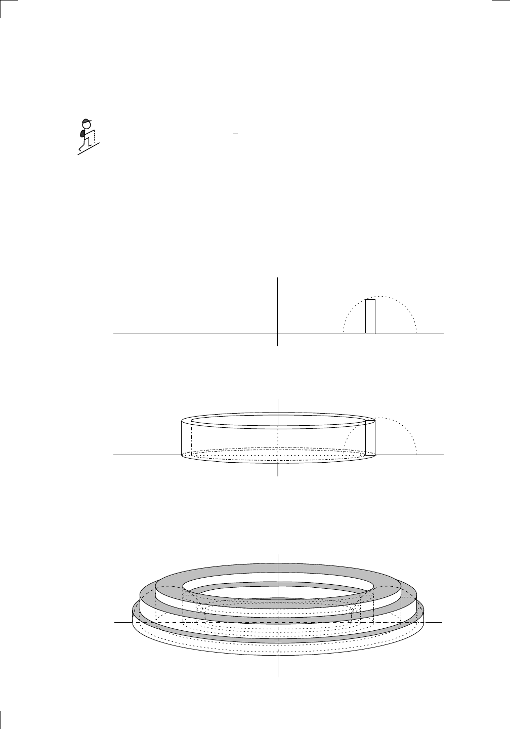
620 • Volumes, Arc Lengths, and Surface Areas
and x goes from 2 to 4, so we have
V =
Z
4
2
πy
2
dx = π
Z
4
2
(1 − (x − 3)
2
) dx.
The volume works out to be
4
3
π cubic units (try it!) which is what we’d expect,
PSfrag
replacements
(
a, b)
[
a, b]
(
a, b]
[
a, b)
(
a, ∞)
[
a, ∞)
(
−∞, b)
(
−∞, b]
(
−∞, ∞)
{
x : a < x < b}
{
x : a ≤ x ≤ b}
{
x : a < x ≤ b}
{
x : a ≤ x < b}
{
x : x ≥ a}
{
x : x > a}
{
x : x ≤ b}
{
x : x < b}
R
a
b
shado
w
0
1
4
−
2
3
−
3
g(
x) = x
2
f(
x) = x
3
g(
x) = x
2
f(
x) = x
3
mirror
(y = x)
f
−
1
(x) =
3
√
x
y = h
(x)
y = h
−
1
(x)
y =
(x − 1)
2
−
1
x
Same
height
−
x
Same
length,
opp
osite signs
y = −
2x
−
2
1
y =
1
2
x − 1
2
−
1
y =
2
x
y =
10
x
y =
2
−x
y =
log
2
(x)
4
3
units
mirror
(x-axis)
y = |
x|
y = |
log
2
(x)|
θ radians
θ units
30
◦
=
π
6
45
◦
=
π
4
60
◦
=
π
3
120
◦
=
2
π
3
135
◦
=
3
π
4
150
◦
=
5
π
6
90
◦
=
π
2
180
◦
= π
210
◦
=
7
π
6
225
◦
=
5
π
4
240
◦
=
4
π
3
270
◦
=
3
π
2
300
◦
=
5
π
3
315
◦
=
7
π
4
330
◦
=
11
π
6
0
◦
=
0 radians
θ
hyp
otenuse
opp
osite
adjacen
t
0
(≡ 2π)
π
2
π
3
π
2
I
I
I
I
II
IV
θ
(
x, y)
x
y
r
7
π
6
reference
angle
reference
angle =
π
6
sin
+
sin −
cos
+
cos −
tan
+
tan −
A
S
T
C
7
π
4
9
π
13
5
π
6
(this
angle is
5π
6
clo
ckwise)
1
2
1
2
3
4
5
6
0
−
1
−
2
−
3
−
4
−
5
−
6
−
3π
−
5
π
2
−
2π
−
3
π
2
−
π
−
π
2
3
π
3
π
5
π
2
2
π
3
π
2
π
π
2
y =
sin(x)
1
0
−
1
−
3π
−
5
π
2
−
2π
−
3
π
2
−
π
−
π
2
3
π
5
π
2
2
π
2
π
3
π
2
π
π
2
y =
sin(x)
y =
cos(x)
−
π
2
π
2
y =
tan(x), −
π
2
<
x <
π
2
0
−
π
2
π
2
y =
tan(x)
−
2π
−
3π
−
5
π
2
−
3
π
2
−
π
−
π
2
π
2
3
π
3
π
5
π
2
2
π
3
π
2
π
y =
sec(x)
y =
csc(x)
y =
cot(x)
y = f(
x)
−
1
1
2
y = g(
x)
3
y = h
(x)
4
5
−
2
f(
x) =
1
x
g(
x) =
1
x
2
etc.
0
1
π
1
2
π
1
3
π
1
4
π
1
5
π
1
6
π
1
7
π
g(
x) = sin
1
x
1
0
−
1
L
10
100
200
y =
π
2
y = −
π
2
y =
tan
−1
(x)
π
2
π
y =
sin(
x)
x
,
x > 3
0
1
−
1
a
L
f(
x) = x sin (1/x)
(0 <
x < 0.3)
h
(x) = x
g(
x) = −x
a
L
lim
x
→a
+
f(x) = L
lim
x
→a
+
f(x) = ∞
lim
x
→a
+
f(x) = −∞
lim
x
→a
+
f(x) DNE
lim
x
→a
−
f(x) = L
lim
x
→a
−
f(x) = ∞
lim
x
→a
−
f(x) = −∞
lim
x
→a
−
f(x) DNE
M
}
lim
x
→a
−
f(x) = M
lim
x
→a
f(x) = L
lim
x
→a
f(x) DNE
lim
x
→∞
f(x) = L
lim
x
→∞
f(x) = ∞
lim
x
→∞
f(x) = −∞
lim
x
→∞
f(x) DNE
lim
x
→−∞
f(x) = L
lim
x
→−∞
f(x) = ∞
lim
x
→−∞
f(x) = −∞
lim
x
→−∞
f(x) DNE
lim
x →a
+
f(
x) = ∞
lim
x →a
+
f(
x) = −∞
lim
x →a
−
f(
x) = ∞
lim
x →a
−
f(
x) = −∞
lim
x →a
f(
x) = ∞
lim
x →a
f(
x) = −∞
lim
x →a
f(
x) DNE
y = f (
x)
a
y =
|
x|
x
1
−
1
y =
|
x + 2|
x +
2
1
−
1
−
2
1
2
3
4
a
a
b
y = x sin
1
x
y = x
y = −
x
a
b
c
d
C
a
b
c
d
−
1
0
1
2
3
time
y
t
u
(
t, f(t))
(
u, f(u))
time
y
t
u
y
x
(
x, f(x))
y = |
x|
(
z, f(z))
z
y = f(
x)
a
tangen
t at x = a
b
tangen
t at x = b
c
tangen
t at x = c
y = x
2
tangen
t
at x = −
1
u
v
uv
u +
∆u
v +
∆v
(
u + ∆u)(v + ∆v)
∆
u
∆
v
u
∆v
v∆
u
∆
u∆v
y = f(
x)
1
2
−
2
y = |
x
2
− 4|
y = x
2
− 4
y = −
2x + 5
y = g(
x)
1
2
3
4
5
6
7
8
9
0
−
1
−
2
−
3
−
4
−
5
−
6
y = f (
x)
3
−
3
3
−
3
0
−
1
2
easy
hard
flat
y = f
0
(
x)
3
−
3
0
−
1
2
1
−
1
y =
sin(x)
y = x
x
A
B
O
1
C
D
sin(
x)
tan(
x)
y =
sin(
x)
x
π
2
π
1
−
1
x =
0
a =
0
x
> 0
a
> 0
x
< 0
a
< 0
rest
position
+
−
y = x
2
sin
1
x
N
A
B
H
a
b
c
O
H
A
B
C
D
h
r
R
θ
1000
2000
α
β
p
h
y = g(
x) = log
b
(x)
y = f(
x) = b
x
y = e
x
5
10
1
2
3
4
0
−
1
−
2
−
3
−
4
y =
ln(x)
y =
cosh(x)
y =
sinh(x)
y =
tanh(x)
y =
sech(x)
y =
csch(x)
y =
coth(x)
1
−
1
y = f(
x)
original
function
in
verse function
slop
e = 0 at (x, y)
slop
e is infinite at (y, x)
−
108
2
5
1
2
1
2
3
4
5
6
0
−
1
−
2
−
3
−
4
−
5
−
6
−
3π
−
5
π
2
−
2π
−
3
π
2
−
π
−
π
2
3
π
3
π
5
π
2
2
π
3
π
2
π
π
2
y =
sin(x)
1
0
−
1
−
3π
−
5
π
2
−
2π
−
3
π
2
−
π
−
π
2
3
π
5
π
2
2
π
2
π
3
π
2
π
π
2
y =
sin(x)
y =
sin(x), −
π
2
≤ x ≤
π
2
−
2
−
1
0
2
π
2
−
π
2
y =
sin
−1
(x)
y =
cos(x)
π
π
2
y =
cos
−1
(x)
−
π
2
1
x
α
β
y =
tan(x)
y =
tan(x)
1
y =
tan
−1
(x)
y =
sec(x)
y =
sec
−1
(x)
y =
csc
−1
(x)
y =
cot
−1
(x)
1
y =
cosh
−1
(x)
y =
sinh
−1
(x)
y =
tanh
−1
(x)
y =
sech
−1
(x)
y =
csch
−1
(x)
y =
coth
−1
(x)
(0
, 3)
(2
, −1)
(5
, 2)
(7
, 0)
(
−1, 44)
(0
, 1)
(1
, −12)
(2
, 305)
y =
1
2
(2
, 3)
y = f(
x)
y = g(
x)
a
b
c
a
b
c
s
c
0
c
1
(
a, f(a))
(
b, f(b))
1
2
1
2
3
4
5
6
0
−
1
−
2
−
3
−
4
−
5
−
6
−
3π
−
5
π
2
−
2π
−
3
π
2
−
π
−
π
2
3
π
3
π
5
π
2
2
π
3
π
2
π
π
2
y =
sin(x)
1
0
−
1
−
3π
−
5
π
2
−
2π
−
3
π
2
−
π
−
π
2
3
π
5
π
2
2
π
2
π
3
π
2
π
π
2
c
OR
Lo
cal maximum
Lo
cal minimum
Horizon
tal point of inflection
1
e
y = f
0
(
x)
y = f (
x) = x ln(x)
−
1
e
?
y = f(
x) = x
3
y = g(
x) = x
4
x
f(
x)
−
3
−
2
−
1
0
1
2
1
2
3
4
+
−
?
1
5
6
3
f
0
(
x)
2 −
1
2
√
6
2
+
1
2
√
6
f
00
(
x)
7
8
g
00
(
x)
f
00
(
x)
0
y =
(
x − 3)(x − 1)
2
x
3
(
x + 2)
y = x ln
(x)
1
e
−
1
e
5
−
108
2
α
β
2 −
1
2
√
6
2
+
1
2
√
6
y = x
2
(
x − 5)
3
−
e
−
1/2
√
3
e
−
1/2
√
3
−
e
−3/2
e
−
3/2
−
1
√
3
1
√
3
−
1
1
y = xe
−
3x
2
/2
y =
x
3
− 6
x
2
+ 13x − 8
x
28
2
600
500
400
300
200
100
0
−
100
−
200
−
300
−
400
−
500
−
600
0
10
−
10
5
−
5
20
−
20
15
−
15
0
4
5
6
x
P
0
(
x)
+
−
−
existing
fence
new
fence
enclosure
A
h
b
H
99
100
101
h
dA/dh
r
h
1
2
7
shallo
w
deep
LAND
SEA
N
y
z
s
t
3
11
9
L
(11)
√
11
y = L
(x)
y = f (
x)
11
y = L
(x)
y = f(
x)
F
P
a
a +
∆x
f(
a + ∆x)
L
(a + ∆x)
f(
a)
error
d
f
∆
x
a
b
y = f(
x)
true
zero
starting
approximation
b
etter approximation
v
t
3
5
50
40
60
4
20
30
25
t
1
t
2
t
3
t
4
t
n
−2
t
n
−1
t
0
= a
t
n
= b
v
1
v
2
v
3
v
4
v
n
−1
v
n
−
30
6
30
|
v|
a
b
p
q
c
v(
c)
v(
c
1
)
v(
c
2
)
v(
c
3
)
v(
c
4
)
v(
c
5
)
v(
c
6
)
t
1
t
2
t
3
t
4
t
5
c
1
c
2
c
3
c
4
c
5
c
6
t
0
=
a
t
6
=
b
t
16
=
b
t
10
=
b
a
b
x
y
y = f(
x)
1
2
y = x
5
0
−
2
y =
1
a
b
y =
sin(x)
π
−
π
0
−
1
−
2
0
2
4
y = x
2
0
1
2
3
4
2
n
4
n
6
n
2(
n−2)
n
2(
n−1)
n
2
n
n
=
2
width
of each interval =
2
n
−
2
1
3
0
I
I
I
I
II
IV
4
y
dx
y = −
x
2
− 2x + 3
3
−
5
y = |−
x
2
− 2x + 3|
I
I
I
I
Ia
5
3
0
1
2
a
b
y = f (
x)
y = g(
x)
y = x
2
a
b
5
3
0
1
2
y =
√
x
2
√
2
2
2
dy
x
2
a
b
y = f(
x)
y = g(
x)
M
m
1
2
−
1
−
2
0
y = e
−
x
2
1
2
e
−
1/4
f
a
v
y = f
a
v
c
A
M
0
1
2
a
b
x
t
y = f (
t)
F (
x )
y = f (
t)
F (
x + h)
x + h
F (
x + h) − F (x)
f(
x)
1
2
y =
sin(x)
π
−
π
−
1
−
2
y =
1
x
y = x
2
1
2
1
−
1
y =
ln|x|
θ
a
x
a
x
p
a
2
− x
2
3
x
p
9 − x
2
p
x
2
+ a
2
x
a
p
x
2
+ 15
x
√
15
x
p
x
2
− a
2
a
x
p
x
2
− 4
2
x
−
p
x
2
− a
2
a
x
−
p
x
2
− 4
2
y = f(
x)
a
b
a + ε
ε
Z
b
a
+ε
f(x) dx
small
ev
en smaller
y = g(
x)
infinite
area
finite
area
1
y =
1
x
y =
1
x
p
, p
< 1 (typical)
y =
1
x
p
, p
> 1 (typical)
a
1
a
2
a
3
a
4
a
5
a
6
a
7
a
8
1
2
3
4
5
6
7
8
n
a
n
x
y
y = f(
x)
(
a, f(a))
a
−
1
0
1
a
6
1
2
7
1
2
7
?
−
2
−
1
−
2
t =
0
t = π
/6
t = π
/4
t = π
/3
t = π
/2
3
0
t = −
2
t = −
3/2
t = ±
1
t = −
1/2
t =
0
t =
1/2
t =
3/2
t =
2
12
−
12
θ
r
P
θ
r
P
11
π
6
2
(
−1, −1)
wrong
point
π
4
5
π
4
√
2
(0
, 1)
(0
, −3)
(
−2, 0)
π
2
3
π
2
π
r =
3 sin(θ)
3
π
2
θ
2
π
1
0
−
1
−
2
−
3
0
3
2
−
3
2
0
r =
1 + 2 cos(θ)
2
π
3
4
π
3
0
π
0
pi
−
3
2
3
π
2
1
2
3
0
−
1
−
2
−
3
0 ≤ θ ≤
2
π
3
0 ≤ θ ≤ π
0 ≤ θ ≤ 2
π
r =
1 + cos(θ)
r =
1 +
3
4
cos(
θ)
−
1
4
r =
sin(2θ)
r =
sin(3θ)
r =
1
π
θ
0 ≤ θ ≤ 4
π
r =
2
1
+ sin(θ)
−
π
4
≤ θ ≤
5
π
4
0 ≤ θ ≤ 2
π
0 ≤ θ ≤ π
−
4
−
5
4
5
f(
θ)
f(
θ + dθ)
θ
dθ
θ + dθ
approximating region
exact region
0 ≤ θ ≤ 2π
r = |1 + 2 cos(θ)|
2i
2 − 3i
−1
θ = 0
θ =
π
4
θ =
π
2
θ =
2π
3
θ = π
θ =
13π
12
θ =
3π
2
θ =
7π
4
1 = e
0
e
i
π
4
i = e
i
π
2
e
i
2π
3
−1 = e
iπ
e
i
13π
12
−i = e
i
3π
2
e
i
7π
4
i
−i
1
θ
1 − i
2i
−2i
2
−2
6i
−6i
6
−6
−
√
3
R
ϕ
2
1/5
θ =
π
6
θ =
17π
30
θ =
29π
30
θ =
41π
30
θ =
53π
30
z
0
z
1
z
2
z
3
z
4
−
√
3
2
√
3
2
1
2
i
−i
19π
6
−i
7π
6
i
5π
6
i
17π
6
i
29π
6
ln(2)
−
7π
4
−
3π
4
π
4
5π
4
9π
4
3
2
i
0
1
2
3
4
dx
y
x
y =
p
1 − (x − 3)
2
since we’re dealing with a sphere of radius 1 unit here. The method we just
used is called the disc method; it is also known as the method of slicing.
29.1.2 The shell method
Now, let’s suppose that we take our favorite semicircular region from before
(see page 618 above) but this time we revolve it about the y-axis. Try to
imagine what you’d get—it’s actually the top half of a bagel (without the
poppy seeds). Let’s approximate the semicircle by thin strips again, but this
time we’ll revolve each strip about the y-axis, instead of the x-axis. As we
saw before, a typical strip looks like this:
PSfrag
replacements
(
a, b)
[
a, b]
(
a, b]
[
a, b)
(
a, ∞)
[
a, ∞)
(
−∞, b)
(
−∞, b]
(
−∞, ∞)
{
x : a < x < b}
{
x : a ≤ x ≤ b}
{
x : a < x ≤ b}
{
x : a ≤ x < b}
{
x : x ≥ a}
{
x : x > a}
{
x : x ≤ b}
{
x : x < b}
R
a
b
shado
w
0
1
4
−
2
3
−
3
g(
x) = x
2
f(
x) = x
3
g(
x) = x
2
f(
x) = x
3
mirror
(y = x)
f
−
1
(x) =
3
√
x
y = h
(x)
y = h
−
1
(x)
y =
(x − 1)
2
−
1
x
Same
height
−
x
Same
length,
opp
osite signs
y = −
2x
−
2
1
y =
1
2
x − 1
2
−
1
y =
2
x
y =
10
x
y =
2
−x
y =
log
2
(x)
4
3
units
mirror
(x-axis)
y = |
x|
y = |
log
2
(x)|
θ radians
θ units
30
◦
=
π
6
45
◦
=
π
4
60
◦
=
π
3
120
◦
=
2
π
3
135
◦
=
3
π
4
150
◦
=
5
π
6
90
◦
=
π
2
180
◦
= π
210
◦
=
7
π
6
225
◦
=
5
π
4
240
◦
=
4
π
3
270
◦
=
3
π
2
300
◦
=
5
π
3
315
◦
=
7
π
4
330
◦
=
11
π
6
0
◦
=
0 radians
θ
hyp
otenuse
opp
osite
adjacen
t
0
(≡ 2π)
π
2
π
3
π
2
I
I
I
I
II
IV
θ
(
x, y)
x
y
r
7
π
6
reference
angle
reference
angle =
π
6
sin
+
sin −
cos
+
cos −
tan
+
tan −
A
S
T
C
7
π
4
9
π
13
5
π
6
(this
angle is
5π
6
clo
ckwise)
1
2
1
2
3
4
5
6
0
−
1
−
2
−
3
−
4
−
5
−
6
−
3π
−
5
π
2
−
2π
−
3
π
2
−
π
−
π
2
3
π
3
π
5
π
2
2
π
3
π
2
π
π
2
y =
sin(x)
1
0
−
1
−
3π
−
5
π
2
−
2π
−
3
π
2
−
π
−
π
2
3
π
5
π
2
2
π
2
π
3
π
2
π
π
2
y =
sin(x)
y =
cos(x)
−
π
2
π
2
y =
tan(x), −
π
2
<
x <
π
2
0
−
π
2
π
2
y =
tan(x)
−
2π
−
3π
−
5
π
2
−
3
π
2
−
π
−
π
2
π
2
3
π
3
π
5
π
2
2
π
3
π
2
π
y =
sec(x)
y =
csc(x)
y =
cot(x)
y = f(
x)
−
1
1
2
y = g(
x)
3
y = h
(x)
4
5
−
2
f(
x) =
1
x
g(
x) =
1
x
2
etc.
0
1
π
1
2
π
1
3
π
1
4
π
1
5
π
1
6
π
1
7
π
g(
x) = sin
1
x
1
0
−
1
L
10
100
200
y =
π
2
y = −
π
2
y =
tan
−1
(x)
π
2
π
y =
sin(
x)
x
,
x > 3
0
1
−
1
a
L
f(
x) = x sin (1/x)
(0 <
x < 0.3)
h
(x) = x
g(
x) = −x
a
L
lim
x
→a
+
f(x) = L
lim
x
→a
+
f(x) = ∞
lim
x
→a
+
f(x) = −∞
lim
x
→a
+
f(x) DNE
lim
x
→a
−
f(x) = L
lim
x
→a
−
f(x) = ∞
lim
x
→a
−
f(x) = −∞
lim
x
→a
−
f(x) DNE
M
}
lim
x
→a
−
f(x) = M
lim
x
→a
f(x) = L
lim
x
→a
f(x) DNE
lim
x
→∞
f(x) = L
lim
x
→∞
f(x) = ∞
lim
x
→∞
f(x) = −∞
lim
x
→∞
f(x) DNE
lim
x
→−∞
f(x) = L
lim
x
→−∞
f(x) = ∞
lim
x
→−∞
f(x) = −∞
lim
x
→−∞
f(x) DNE
lim
x →a
+
f(
x) = ∞
lim
x →a
+
f(
x) = −∞
lim
x →a
−
f(
x) = ∞
lim
x →a
−
f(
x) = −∞
lim
x →a
f(
x) = ∞
lim
x →a
f(
x) = −∞
lim
x →a
f(
x) DNE
y = f(
x)
a
y =
|
x|
x
1
−
1
y =
|
x + 2|
x +
2
1
−
1
−
2
1
2
3
4
a
a
b
y = x sin
1
x
y = x
y = −
x
a
b
c
d
C
a
b
c
d
−
1
0
1
2
3
time
y
t
u
(
t, f(t))
(
u, f(u))
time
y
t
u
y
x
(
x, f(x))
y = |
x|
(
z, f(z))
z
y = f(
x)
a
tangen
t at x = a
b
tangen
t at x = b
c
tangen
t at x = c
y = x
2
tangen
t
at x = −
1
u
v
uv
u +
∆u
v +
∆v
(
u + ∆u)(v + ∆v)
∆
u
∆
v
u
∆v
v∆
u
∆
u∆v
y = f(
x)
1
2
−
2
y = |
x
2
− 4|
y = x
2
− 4
y = −
2x + 5
y = g(
x)
1
2
3
4
5
6
7
8
9
0
−
1
−
2
−
3
−
4
−
5
−
6
y = f(
x)
3
−
3
3
−
3
0
−
1
2
easy
hard
flat
y = f
0
(
x)
3
−
3
0
−
1
2
1
−
1
y =
sin(x)
y = x
x
A
B
O
1
C
D
sin(
x)
tan(
x)
y =
sin
(x)
x
π
2
π
1
−
1
x =
0
a =
0
x
> 0
a
> 0
x
< 0
a
< 0
rest
position
+
−
y = x
2
sin
1
x
N
A
B
H
a
b
c
O
H
A
B
C
D
h
r
R
θ
1000
2000
α
β
p
h
y = g(
x) = log
b
(x)
y = f(
x) = b
x
y = e
x
5
10
1
2
3
4
0
−
1
−
2
−
3
−
4
y =
ln(x)
y =
cosh(x)
y =
sinh(x)
y =
tanh(x)
y =
sech(x)
y =
csch(x)
y =
coth(x)
1
−
1
y = f(
x)
original
function
in
verse function
slop
e = 0 at (x, y)
slop
e is infinite at (y, x)
−
108
2
5
1
2
1
2
3
4
5
6
0
−
1
−
2
−
3
−
4
−
5
−
6
−
3π
−
5
π
2
−
2π
−
3
π
2
−
π
−
π
2
3
π
3
π
5
π
2
2
π
3
π
2
π
π
2
y =
sin(x)
1
0
−
1
−
3π
−
5
π
2
−
2π
−
3
π
2
−
π
−
π
2
3
π
5
π
2
2
π
2
π
3
π
2
π
π
2
y =
sin(x)
y =
sin(x), −
π
2
≤ x ≤
π
2
−
2
−
1
0
2
π
2
−
π
2
y =
sin
−1
(x)
y =
cos(x)
π
π
2
y =
cos
−1
(x)
−
π
2
1
x
α
β
y =
tan(x)
y =
tan(x)
1
y =
tan
−1
(x)
y =
sec(x)
y =
sec
−1
(x)
y =
csc
−1
(x)
y =
cot
−1
(x)
1
y =
cosh
−1
(x)
y =
sinh
−1
(x)
y =
tanh
−1
(x)
y =
sech
−1
(x)
y =
csch
−1
(x)
y =
coth
−1
(x)
(0
, 3)
(2
, −1)
(5
, 2)
(7
, 0)
(
−1, 44)
(0
, 1)
(1
, −12)
(2
, 305)
y =
1
2
(2
, 3)
y = f(
x)
y = g(
x)
a
b
c
a
b
c
s
c
0
c
1
(
a, f(a))
(
b, f(b))
1
2
1
2
3
4
5
6
0
−
1
−
2
−
3
−
4
−
5
−
6
−
3π
−
5
π
2
−
2π
−
3
π
2
−
π
−
π
2
3
π
3
π
5
π
2
2
π
3
π
2
π
π
2
y =
sin(x)
1
0
−
1
−
3π
−
5
π
2
−
2π
−
3
π
2
−
π
−
π
2
3
π
5
π
2
2
π
2
π
3
π
2
π
π
2
c
OR
Lo
cal maximum
Lo
cal minimum
Horizon
tal point of inflection
1
e
y = f
0
(
x)
y = f(
x) = x ln(x)
−
1
e
?
y = f (
x) = x
3
y = g(
x) = x
4
x
f(
x)
−
3
−
2
−
1
0
1
2
1
2
3
4
+
−
?
1
5
6
3
f
0
(
x)
2 −
1
2
√
6
2
+
1
2
√
6
f
00
(
x)
7
8
g
00
(
x)
f
00
(
x)
0
y =
(
x − 3)(x − 1)
2
x
3
(
x + 2)
y = x ln(
x)
1
e
−
1
e
5
−
108
2
α
β
2 −
1
2
√
6
2
+
1
2
√
6
y = x
2
(
x − 5)
3
−
e
−
1/2
√
3
e
−
1/2
√
3
−
e
−3/2
e
−
3/2
−
1
√
3
1
√
3
−
1
1
y = xe
−
3x
2
/2
y =
x
3
− 6
x
2
+ 13x − 8
x
28
2
600
500
400
300
200
100
0
−
100
−
200
−
300
−
400
−
500
−
600
0
10
−
10
5
−
5
20
−
20
15
−
15
0
4
5
6
x
P
0
(
x)
+
−
−
existing
fence
new
fence
enclosure
A
h
b
H
99
100
101
h
dA/dh
r
h
1
2
7
shallo
w
deep
LAND
SEA
N
y
z
s
t
3
11
9
L
(11)
√
11
y = L
(x)
y = f(
x)
11
y = L
(x)
y = f(
x)
F
P
a
a +
∆x
f(
a + ∆x)
L
(a + ∆x)
f(
a)
error
d
f
∆
x
a
b
y = f(
x)
true
zero
starting
approximation
b
etter approximation
v
t
3
5
50
40
60
4
20
30
25
t
1
t
2
t
3
t
4
t
n
−2
t
n
−1
t
0
= a
t
n
= b
v
1
v
2
v
3
v
4
v
n
−1
v
n
−
30
6
30
|
v|
a
b
p
q
c
v(
c)
v(
c
1
)
v(
c
2
)
v(
c
3
)
v(
c
4
)
v(
c
5
)
v(
c
6
)
t
1
t
2
t
3
t
4
t
5
c
1
c
2
c
3
c
4
c
5
c
6
t
0
=
a
t
6
=
b
t
16
=
b
t
10
=
b
a
b
x
y
y = f(
x)
1
2
y = x
5
0
−
2
y =
1
a
b
y =
sin(x)
π
−
π
0
−
1
−
2
0
2
4
y = x
2
0
1
2
3
4
2
n
4
n
6
n
2(
n−2)
n
2(
n−1)
n
2
n
n
=
2
width
of each interval =
2
n
−
2
1
3
0
I
I
I
I
II
IV
4
y
dx
y = −
x
2
− 2x + 3
3
−
5
y = |−
x
2
− 2x + 3|
I
I
I
I
Ia
5
3
0
1
2
a
b
y = f (
x)
y = g(
x)
y = x
2
a
b
5
3
0
1
2
y =
√
x
2
√
2
2
2
dy
x
2
a
b
y = f(
x)
y = g(
x)
M
m
1
2
−
1
−
2
0
y = e
−
x
2
1
2
e
−
1/4
f
a
v
y = f
a
v
c
A
M
0
1
2
a
b
x
t
y = f (
t)
F (
x )
y = f (
t)
F (
x + h )
x + h
F (
x + h) − F (x)
f(
x)
1
2
y =
sin(x)
π
−
π
−
1
−
2
y =
1
x
y = x
2
1
2
1
−
1
y =
ln|x|
θ
a
x
a
x
p
a
2
− x
2
3
x
p
9 − x
2
p
x
2
+ a
2
x
a
p
x
2
+ 15
x
√
15
x
p
x
2
− a
2
a
x
p
x
2
− 4
2
x
−
p
x
2
− a
2
a
x
−
p
x
2
− 4
2
y = f(
x)
a
b
a + ε
ε
Z
b
a
+ε
f(x) dx
small
ev
en smaller
y = g(
x)
infinite
area
finite
area
1
y =
1
x
y =
1
x
p
, p
< 1 (typical)
y =
1
x
p
, p
> 1 (typical)
a
1
a
2
a
3
a
4
a
5
a
6
a
7
a
8
1
2
3
4
5
6
7
8
n
a
n
x
y
y = f(
x)
(
a, f(a))
a
−
1
0
1
a
6
1
2
7
1
2
7
?
−
2
−
1
−
2
t =
0
t = π
/6
t = π
/4
t = π
/3
t = π
/2
3
0
t = −
2
t = −
3/2
t = ±
1
t = −
1/2
t =
0
t =
1/2
t =
3/2
t =
2
12
−
12
θ
r
P
θ
r
P
11
π
6
2
(
−1, −1)
wrong
point
π
4
5
π
4
√
2
(0
, 1)
(0
, −3)
(
−2, 0)
π
2
3
π
2
π
r =
3 sin(θ)
3
π
2
θ
2
π
1
0
−
1
−
2
−
3
0
3
2
−
3
2
0
r =
1 + 2 cos(θ)
2
π
3
4
π
3
0
π
0
pi
−
3
2
3
π
2
1
2
3
0
−
1
−
2
−
3
0 ≤ θ ≤
2
π
3
0 ≤ θ ≤ π
0 ≤ θ ≤ 2
π
r =
1 + cos(θ)
r =
1 +
3
4
cos
(θ)
−
1
4
r =
sin(2θ)
r =
sin(3θ)
r =
1
π
θ
0 ≤ θ ≤ 4π
r =
2
1 + sin(θ)
−
π
4
≤ θ ≤
5π
4
0 ≤ θ ≤ 2π
0 ≤ θ ≤ π
−4
−5
4
5
f(θ)
f(θ + dθ)
θ
dθ
θ + dθ
approximating region
exact region
0 ≤ θ ≤ 2π
r = |1 + 2 cos(θ)|
2i
2 − 3i
−1
θ = 0
θ =
π
4
θ =
π
2
θ =
2π
3
θ = π
θ =
13π
12
θ =
3π
2
θ =
7π
4
1 = e
0
e
i
π
4
i = e
i
π
2
e
i
2π
3
−1 = e
iπ
e
i
13π
12
−i = e
i
3π
2
e
i
7π
4
i
−i
1
θ
1 − i
2i
−2i
2
−2
6i
−6i
6
−6
−
√
3
R
ϕ
2
1/5
θ =
π
6
θ =
17π
30
θ =
29π
30
θ =
41π
30
θ =
53π
30
z
0
z
1
z
2
z
3
z
4
−
√
3
2
√
3
2
1
2
i
−i
19π
6
−i
7π
6
i
5π
6
i
17π
6
i
29π
6
ln(2)
−
7π
4
−
3π
4
π
4
5π
4
9π
4
3
2
i
0
1
2
3
4
dx
y
x
y =
p
1 − (x − 3)
2
When you revolve it about the y-axis, you don’t get a disc—you get a cylin-
drical shell:
.
PSfrag
replacements
(
a, b)
[
a, b]
(
a, b]
[
a, b)
(
a, ∞)
[
a, ∞)
(
−∞, b)
(
−∞, b]
(
−∞, ∞)
{
x : a < x < b}
{
x : a ≤ x ≤ b}
{
x : a < x ≤ b}
{
x : a ≤ x < b}
{
x : x ≥ a}
{
x : x > a}
{
x : x ≤ b}
{
x : x < b}
R
a
b
shado
w
0
1
4
−
2
3
−
3
g(
x) = x
2
f(
x) = x
3
g(
x) = x
2
f(
x) = x
3
mirror
(y = x)
f
−
1
(x) =
3
√
x
y = h
(x)
y = h
−
1
(x)
y =
(x − 1)
2
−
1
x
Same
height
−
x
Same
length,
opp
osite signs
y = −
2x
−
2
1
y =
1
2
x − 1
2
−
1
y =
2
x
y =
10
x
y =
2
−x
y =
log
2
(x)
4
3
units
mirror
(x-axis)
y = |
x|
y = |
log
2
(x)|
θ radians
θ units
30
◦
=
π
6
45
◦
=
π
4
60
◦
=
π
3
120
◦
=
2
π
3
135
◦
=
3
π
4
150
◦
=
5
π
6
90
◦
=
π
2
180
◦
= π
210
◦
=
7
π
6
225
◦
=
5
π
4
240
◦
=
4
π
3
270
◦
=
3
π
2
300
◦
=
5
π
3
315
◦
=
7
π
4
330
◦
=
11
π
6
0
◦
=
0 radians
θ
hyp
otenuse
opp
osite
adjacen
t
0
(≡ 2π)
π
2
π
3
π
2
I
I
I
I
II
IV
θ
(
x, y)
x
y
r
7
π
6
reference
angle
reference
angle =
π
6
sin
+
sin −
cos
+
cos −
tan
+
tan −
A
S
T
C
7
π
4
9
π
13
5
π
6
(this
angle is
5π
6
clo
ckwise)
1
2
1
2
3
4
5
6
0
−
1
−
2
−
3
−
4
−
5
−
6
−
3π
−
5
π
2
−
2π
−
3
π
2
−
π
−
π
2
3
π
3
π
5
π
2
2
π
3
π
2
π
π
2
y =
sin(x)
1
0
−
1
−
3π
−
5
π
2
−
2π
−
3
π
2
−
π
−
π
2
3
π
5
π
2
2
π
2
π
3
π
2
π
π
2
y =
sin(x)
y =
cos(x)
−
π
2
π
2
y =
tan(x), −
π
2
<
x <
π
2
0
−
π
2
π
2
y =
tan(x)
−
2π
−
3π
−
5
π
2
−
3
π
2
−
π
−
π
2
π
2
3
π
3
π
5
π
2
2
π
3
π
2
π
y =
sec(x)
y =
csc(x)
y =
cot(x)
y = f(
x)
−
1
1
2
y = g(
x)
3
y = h
(x)
4
5
−
2
f(
x) =
1
x
g(
x) =
1
x
2
etc.
0
1
π
1
2
π
1
3
π
1
4
π
1
5
π
1
6
π
1
7
π
g(
x) = sin
1
x
1
0
−
1
L
10
100
200
y =
π
2
y = −
π
2
y =
tan
−1
(x)
π
2
π
y =
sin(
x)
x
,
x > 3
0
1
−
1
a
L
f(
x) = x sin (1/x)
(0 <
x < 0.3)
h
(x) = x
g(
x) = −x
a
L
lim
x
→a
+
f(x) = L
lim
x
→a
+
f(x) = ∞
lim
x
→a
+
f(x) = −∞
lim
x
→a
+
f(x) DNE
lim
x
→a
−
f(x) = L
lim
x
→a
−
f(x) = ∞
lim
x
→a
−
f(x) = −∞
lim
x
→a
−
f(x) DNE
M
}
lim
x
→a
−
f(x) = M
lim
x
→a
f(x) = L
lim
x
→a
f(x) DNE
lim
x
→∞
f(x) = L
lim
x
→∞
f(x) = ∞
lim
x
→∞
f(x) = −∞
lim
x
→∞
f(x) DNE
lim
x
→−∞
f(x) = L
lim
x
→−∞
f(x) = ∞
lim
x
→−∞
f(x) = −∞
lim
x
→−∞
f(x) DNE
lim
x →a
+
f(
x) = ∞
lim
x →a
+
f(
x) = −∞
lim
x →a
−
f(
x) = ∞
lim
x →a
−
f(
x) = −∞
lim
x →a
f(
x) = ∞
lim
x →a
f(
x) = −∞
lim
x →a
f(
x) DNE
y = f(
x)
a
y =
|
x|
x
1
−
1
y =
|
x + 2|
x +
2
1
−
1
−
2
1
2
3
4
a
a
b
y = x sin
1
x
y = x
y = −
x
a
b
c
d
C
a
b
c
d
−
1
0
1
2
3
time
y
t
u
(
t, f(t))
(
u, f(u))
time
y
t
u
y
x
(
x, f(x))
y = |
x|
(
z, f(z))
z
y = f(
x)
a
tangen
t at x = a
b
tangen
t at x = b
c
tangen
t at x = c
y = x
2
tangen
t
at x = −
1
u
v
uv
u +
∆u
v +
∆v
(
u + ∆u)(v + ∆v)
∆
u
∆
v
u
∆v
v∆
u
∆
u∆v
y = f(
x)
1
2
−
2
y = |
x
2
− 4|
y = x
2
− 4
y = −
2x + 5
y = g(
x)
1
2
3
4
5
6
7
8
9
0
−
1
−
2
−
3
−
4
−
5
−
6
y = f(
x)
3
−
3
3
−
3
0
−
1
2
easy
hard
flat
y = f
0
(
x)
3
−
3
0
−
1
2
1
−
1
y =
sin(x)
y = x
x
A
B
O
1
C
D
sin(
x)
tan(
x)
y =
sin
(x)
x
π
2
π
1
−
1
x =
0
a =
0
x
> 0
a
> 0
x
< 0
a
< 0
rest
position
+
−
y = x
2
sin
1
x
N
A
B
H
a
b
c
O
H
A
B
C
D
h
r
R
θ
1000
2000
α
β
p
h
y = g(
x) = log
b
(x)
y = f(
x) = b
x
y = e
x
5
10
1
2
3
4
0
−
1
−
2
−
3
−
4
y =
ln(x)
y =
cosh(x)
y =
sinh(x)
y =
tanh(x)
y =
sech(x)
y =
csch(x)
y =
coth(x)
1
−
1
y = f(
x)
original
function
in
verse function
slop
e = 0 at (x, y)
slop
e is infinite at (y, x)
−
108
2
5
1
2
1
2
3
4
5
6
0
−
1
−
2
−
3
−
4
−
5
−
6
−
3π
−
5
π
2
−
2π
−
3
π
2
−
π
−
π
2
3
π
3
π
5
π
2
2
π
3
π
2
π
π
2
y =
sin(x)
1
0
−
1
−
3π
−
5
π
2
−
2π
−
3
π
2
−
π
−
π
2
3
π
5
π
2
2
π
2
π
3
π
2
π
π
2
y =
sin(x)
y =
sin(x), −
π
2
≤ x ≤
π
2
−
2
−
1
0
2
π
2
−
π
2
y =
sin
−1
(x)
y =
cos(x)
π
π
2
y =
cos
−1
(x)
−
π
2
1
x
α
β
y =
tan(x)
y =
tan(x)
1
y =
tan
−1
(x)
y =
sec(x)
y =
sec
−1
(x)
y =
csc
−1
(x)
y =
cot
−1
(x)
1
y =
cosh
−1
(x)
y =
sinh
−1
(x)
y =
tanh
−1
(x)
y =
sech
−1
(x)
y =
csch
−1
(x)
y =
coth
−1
(x)
(0
, 3)
(2
, −1)
(5
, 2)
(7
, 0)
(
−1, 44)
(0
, 1)
(1
, −12)
(2
, 305)
y =
1
2
(2
, 3)
y = f(
x)
y = g(
x)
a
b
c
a
b
c
s
c
0
c
1
(
a, f(a))
(
b, f(b))
1
2
1
2
3
4
5
6
0
−
1
−
2
−
3
−
4
−
5
−
6
−
3π
−
5
π
2
−
2π
−
3
π
2
−
π
−
π
2
3
π
3
π
5
π
2
2
π
3
π
2
π
π
2
y =
sin(x)
1
0
−
1
−
3π
−
5
π
2
−
2π
−
3
π
2
−
π
−
π
2
3
π
5
π
2
2
π
2
π
3
π
2
π
π
2
c
OR
Lo
cal maximum
Lo
cal minimum
Horizon
tal point of inflection
1
e
y = f
0
(
x)
y = f(
x) = x ln(x)
−
1
e
?
y = f (
x) = x
3
y = g(
x) = x
4
x
f(
x)
−
3
−
2
−
1
0
1
2
1
2
3
4
+
−
?
1
5
6
3
f
0
(
x)
2 −
1
2
√
6
2
+
1
2
√
6
f
00
(
x)
7
8
g
00
(
x)
f
00
(
x)
0
y =
(
x − 3)(x − 1)
2
x
3
(
x + 2)
y = x ln(
x)
1
e
−
1
e
5
−
108
2
α
β
2 −
1
2
√
6
2
+
1
2
√
6
y = x
2
(
x − 5)
3
−
e
−
1/2
√
3
e
−
1/2
√
3
−
e
−3/2
e
−
3/2
−
1
√
3
1
√
3
−
1
1
y = xe
−
3x
2
/2
y =
x
3
− 6
x
2
+ 13x − 8
x
28
2
600
500
400
300
200
100
0
−
100
−
200
−
300
−
400
−
500
−
600
0
10
−
10
5
−
5
20
−
20
15
−
15
0
4
5
6
x
P
0
(
x)
+
−
−
existing
fence
new
fence
enclosure
A
h
b
H
99
100
101
h
dA/dh
r
h
1
2
7
shallo
w
deep
LAND
SEA
N
y
z
s
t
3
11
9
L
(11)
√
11
y = L
(x)
y = f(
x)
11
y = L
(x)
y = f(
x)
F
P
a
a +
∆x
f(
a + ∆x)
L
(a + ∆x)
f(
a)
error
d
f
∆
x
a
b
y = f(
x)
true
zero
starting
approximation
b
etter approximation
v
t
3
5
50
40
60
4
20
30
25
t
1
t
2
t
3
t
4
t
n
−2
t
n
−1
t
0
= a
t
n
= b
v
1
v
2
v
3
v
4
v
n
−1
v
n
−
30
6
30
|
v|
a
b
p
q
c
v(
c)
v(
c
1
)
v(
c
2
)
v(
c
3
)
v(
c
4
)
v(
c
5
)
v(
c
6
)
t
1
t
2
t
3
t
4
t
5
c
1
c
2
c
3
c
4
c
5
c
6
t
0
=
a
t
6
=
b
t
16
=
b
t
10
=
b
a
b
x
y
y = f(
x)
1
2
y = x
5
0
−
2
y =
1
a
b
y =
sin(x)
π
−
π
0
−
1
−
2
0
2
4
y = x
2
0
1
2
3
4
2
n
4
n
6
n
2(
n−2)
n
2(
n−1)
n
2
n
n
=
2
width
of each interval =
2
n
−
2
1
3
0
I
I
I
I
II
IV
4
y
dx
y = −
x
2
− 2x + 3
3
−
5
y = |−
x
2
− 2x + 3|
I
I
I
I
Ia
5
3
0
1
2
a
b
y = f (
x)
y = g(
x)
y = x
2
a
b
5
3
0
1
2
y =
√
x
2
√
2
2
2
dy
x
2
a
b
y = f(
x)
y = g(
x)
M
m
1
2
−
1
−
2
0
y = e
−
x
2
1
2
e
−
1/4
f
a
v
y = f
a
v
c
A
M
0
1
2
a
b
x
t
y = f (
t)
F (
x )
y = f (
t)
F (
x + h )
x + h
F (
x + h) − F (x)
f(
x)
1
2
y =
sin(x)
π
−
π
−
1
−
2
y =
1
x
y = x
2
1
2
1
−
1
y =
ln|x|
θ
a
x
a
x
p
a
2
− x
2
3
x
p
9 − x
2
p
x
2
+ a
2
x
a
p
x
2
+ 15
x
√
15
x
p
x
2
− a
2
a
x
p
x
2
− 4
2
x
−
p
x
2
− a
2
a
x
−
p
x
2
− 4
2
y = f(
x)
a
b
a + ε
ε
Z
b
a
+ε
f(x) dx
small
ev
en smaller
y = g(
x)
infinite
area
finite
area
1
y =
1
x
y =
1
x
p
, p
< 1 (typical)
y =
1
x
p
, p
> 1 (typical)
a
1
a
2
a
3
a
4
a
5
a
6
a
7
a
8
1
2
3
4
5
6
7
8
n
a
n
x
y
y = f(
x)
(
a, f(a))
a
−
1
0
1
a
6
1
2
7
1
2
7
?
−
2
−
1
−
2
t =
0
t = π
/6
t = π
/4
t = π
/3
t = π
/2
3
0
t = −
2
t = −
3/2
t = ±
1
t = −
1/2
t =
0
t =
1/2
t =
3/2
t =
2
12
−
12
θ
r
P
θ
r
P
11
π
6
2
(
−1, −1)
wrong
point
π
4
5
π
4
√
2
(0
, 1)
(0
, −3)
(
−2, 0)
π
2
3
π
2
π
r =
3 sin(θ)
3
π
2
θ
2
π
1
0
−
1
−
2
−
3
0
3
2
−
3
2
0
r =
1 + 2 cos(θ)
2
π
3
4
π
3
0
π
0
pi
−
3
2
3
π
2
1
2
3
0
−
1
−
2
−
3
0 ≤ θ ≤
2
π
3
0 ≤ θ ≤ π
0 ≤ θ ≤ 2π
r = 1 + cos(θ)
r = 1 +
3
4
cos(θ)
−
1
4
r = sin(2θ)
r = sin(3θ)
r =
1
π
θ
0 ≤ θ ≤ 4π
r =
2
1 + sin(θ)
−
π
4
≤ θ ≤
5π
4
0 ≤ θ ≤ 2π
0 ≤ θ ≤ π
−4
−5
4
5
f(θ)
f(θ + dθ)
θ
dθ
θ + dθ
approximating region
exact region
0 ≤ θ ≤ 2π
r = |1 + 2 cos(θ)|
2i
2 − 3i
−1
θ = 0
θ =
π
4
θ =
π
2
θ =
2π
3
θ = π
θ =
13π
12
θ =
3π
2
θ =
7π
4
1 = e
0
e
i
π
4
i = e
i
π
2
e
i
2π
3
−1 = e
iπ
e
i
13π
12
−i = e
i
3π
2
e
i
7π
4
i
−i
1
θ
1 − i
2i
−2i
2
−2
6i
−6i
6
−6
−
√
3
R
ϕ
2
1/5
θ =
π
6
θ =
17π
30
θ =
29π
30
θ =
41π
30
θ =
53π
30
z
0
z
1
z
2
z
3
z
4
−
√
3
2
√
3
2
1
2
i
−i
19π
6
−i
7π
6
i
5π
6
i
17π
6
i
29π
6
ln(2)
−
7π
4
−
3π
4
π
4
5π
4
9π
4
3
2
i
0
1
2
3
4
dx
y
x
y =
p
1 − (x − 3)
2
We’re going to approximate our bagel half by using a number of shells, then
letting the maximum shell thickness decrease to zero. For example, if you use
five strips to approximate the region (as we did in the previous section), you
might get something like this:
PSfrag
replacements
(
a, b)
[
a, b]
(
a, b]
[
a, b)
(
a, ∞)
[
a, ∞)
(
−∞, b)
(
−∞, b]
(
−∞, ∞)
{
x : a < x < b}
{
x : a ≤ x ≤ b}
{
x : a < x ≤ b}
{
x : a ≤ x < b}
{
x : x ≥ a}
{
x : x > a}
{
x : x ≤ b}
{
x : x < b}
R
a
b
shado
w
0
1
4
−
2
3
−
3
g(
x) = x
2
f(
x) = x
3
g(
x) = x
2
f(
x) = x
3
mirror
(y = x)
f
−
1
(x) =
3
√
x
y = h
(x)
y = h
−
1
(x)
y =
(x − 1)
2
−
1
x
Same
height
−
x
Same
length,
opp
osite signs
y = −
2x
−
2
1
y =
1
2
x − 1
2
−
1
y =
2
x
y =
10
x
y =
2
−x
y =
log
2
(x)
4
3
units
mirror
(x-axis)
y = |
x|
y = |
log
2
(x)|
θ radians
θ units
30
◦
=
π
6
45
◦
=
π
4
60
◦
=
π
3
120
◦
=
2
π
3
135
◦
=
3
π
4
150
◦
=
5
π
6
90
◦
=
π
2
180
◦
= π
210
◦
=
7
π
6
225
◦
=
5
π
4
240
◦
=
4
π
3
270
◦
=
3
π
2
300
◦
=
5
π
3
315
◦
=
7
π
4
330
◦
=
11
π
6
0
◦
=
0 radians
θ
hyp
otenuse
opp
osite
adjacen
t
0
(≡ 2π)
π
2
π
3
π
2
I
I
I
I
II
IV
θ
(
x, y)
x
y
r
7
π
6
reference
angle
reference
angle =
π
6
sin
+
sin −
cos
+
cos −
tan
+
tan −
A
S
T
C
7
π
4
9
π
13
5
π
6
(this
angle is
5π
6
clo
ckwise)
1
2
1
2
3
4
5
6
0
−
1
−
2
−
3
−
4
−
5
−
6
−
3π
−
5
π
2
−
2π
−
3
π
2
−
π
−
π
2
3
π
3
π
5
π
2
2
π
3
π
2
π
π
2
y =
sin(x)
1
0
−
1
−
3π
−
5
π
2
−
2π
−
3
π
2
−
π
−
π
2
3
π
5
π
2
2
π
2
π
3
π
2
π
π
2
y =
sin(x)
y =
cos(x)
−
π
2
π
2
y =
tan(x), −
π
2
<
x <
π
2
0
−
π
2
π
2
y =
tan(x)
−
2π
−
3π
−
5
π
2
−
3
π
2
−
π
−
π
2
π
2
3
π
3
π
5
π
2
2
π
3
π
2
π
y =
sec(x)
y =
csc(x)
y =
cot(x)
y = f (
x)
−
1
1
2
y = g(
x)
3
y = h
(x)
4
5
−
2
f(
x) =
1
x
g(
x) =
1
x
2
etc.
0
1
π
1
2
π
1
3
π
1
4
π
1
5
π
1
6
π
1
7
π
g(
x) = sin
1
x
1
0
−
1
L
10
100
200
y =
π
2
y = −
π
2
y =
tan
−1
(x)
π
2
π
y =
sin
(x)
x
,
x > 3
0
1
−
1
a
L
f(
x) = x sin (1/x)
(0 <
x < 0.3)
h
(x) = x
g(
x) = −x
a
L
lim
x
→a
+
f(x) = L
lim
x
→a
+
f(x) = ∞
lim
x
→a
+
f(x) = −∞
lim
x
→a
+
f(x) DNE
lim
x
→a
−
f(x) = L
lim
x
→a
−
f(x) = ∞
lim
x
→a
−
f(x) = −∞
lim
x
→a
−
f(x) DNE
M
}
lim
x
→a
−
f(x) = M
lim
x
→a
f(x) = L
lim
x
→a
f(x) DNE
lim
x
→∞
f(x) = L
lim
x
→∞
f(x) = ∞
lim
x
→∞
f(x) = −∞
lim
x
→∞
f(x) DNE
lim
x
→−∞
f(x) = L
lim
x
→−∞
f(x) = ∞
lim
x
→−∞
f(x) = −∞
lim
x
→−∞
f(x) DNE
lim
x →a
+
f(
x) = ∞
lim
x →a
+
f(
x) = −∞
lim
x →a
−
f(
x) = ∞
lim
x →a
−
f(
x) = −∞
lim
x →a
f(
x) = ∞
lim
x →a
f(
x) = −∞
lim
x →a
f(
x) DNE
y = f (
x)
a
y =
|
x|
x
1
−
1
y =
|
x + 2|
x +
2
1
−
1
−
2
1
2
3
4
a
a
b
y = x sin
1
x
y = x
y = −
x
a
b
c
d
C
a
b
c
d
−
1
0
1
2
3
time
y
t
u
(
t, f(t))
(
u, f(u))
time
y
t
u
y
x
(
x, f(x))
y = |
x|
(
z, f(z))
z
y = f (
x)
a
tangen
t at x = a
b
tangen
t at x = b
c
tangen
t at x = c
y = x
2
tangen
t
at x = −
1
u
v
uv
u +
∆u
v +
∆v
(
u + ∆u)(v + ∆v)
∆
u
∆
v
u
∆v
v∆
u
∆
u∆v
y = f (
x)
1
2
−
2
y = |
x
2
− 4|
y = x
2
− 4
y = −
2x + 5
y = g(
x)
1
2
3
4
5
6
7
8
9
0
−
1
−
2
−
3
−
4
−
5
−
6
y = f(
x)
3
−
3
3
−
3
0
−
1
2
easy
hard
flat
y = f
0
(
x)
3
−
3
0
−
1
2
1
−
1
y =
sin(x)
y = x
x
A
B
O
1
C
D
sin(
x)
tan(
x)
y =
sin
(x)
x
π
2
π
1
−
1
x =
0
a =
0
x
> 0
a
> 0
x
< 0
a
< 0
rest
position
+
−
y = x
2
sin
1
x
N
A
B
H
a
b
c
O
H
A
B
C
D
h
r
R
θ
1000
2000
α
β
p
h
y = g(
x) = log
b
(x)
y = f (
x) = b
x
y = e
x
5
10
1
2
3
4
0
−
1
−
2
−
3
−
4
y =
ln(x)
y =
cosh(x)
y =
sinh(x)
y =
tanh(x)
y =
sech(x)
y =
csch(x)
y =
coth(x)
1
−
1
y = f (
x)
original
function
in
verse function
slop
e = 0 at (x, y)
slop
e is infinite at (y, x)
−
108
2
5
1
2
1
2
3
4
5
6
0
−
1
−
2
−
3
−
4
−
5
−
6
−
3π
−
5
π
2
−
2π
−
3
π
2
−
π
−
π
2
3
π
3
π
5
π
2
2
π
3
π
2
π
π
2
y =
sin(x)
1
0
−
1
−
3π
−
5
π
2
−
2π
−
3
π
2
−
π
−
π
2
3
π
5
π
2
2
π
2
π
3
π
2
π
π
2
y =
sin(x)
y =
sin(x), −
π
2
≤ x ≤
π
2
−
2
−
1
0
2
π
2
−
π
2
y =
sin
−1
(x)
y =
cos(x)
π
π
2
y =
cos
−1
(x)
−
π
2
1
x
α
β
y =
tan(x)
y =
tan(x)
1
y =
tan
−1
(x)
y =
sec(x)
y =
sec
−1
(x)
y =
csc
−1
(x)
y =
cot
−1
(x)
1
y =
cosh
−1
(x)
y =
sinh
−1
(x)
y =
tanh
−1
(x)
y =
sech
−1
(x)
y =
csch
−1
(x)
y =
coth
−1
(x)
(0
, 3)
(2
, −1)
(5
, 2)
(7
, 0)
(
−1, 44)
(0
, 1)
(1
, −12)
(2
, 305)
y =
1
2
(2
, 3)
y = f (
x)
y = g(
x)
a
b
c
a
b
c
s
c
0
c
1
(
a, f(a))
(
b, f(b))
1
2
1
2
3
4
5
6
0
−
1
−
2
−
3
−
4
−
5
−
6
−
3π
−
5
π
2
−
2π
−
3
π
2
−
π
−
π
2
3
π
3
π
5
π
2
2
π
3
π
2
π
π
2
y =
sin(x)
1
0
−
1
−
3π
−
5
π
2
−
2π
−
3
π
2
−
π
−
π
2
3
π
5
π
2
2
π
2
π
3
π
2
π
π
2
c
OR
Lo
cal maximum
Lo
cal minimum
Horizon
tal point of inflection
1
e
y = f
0
(
x)
y = f(
x) = x ln(x)
−
1
e
?
y = f(
x) = x
3
y = g(
x) = x
4
x
f(
x)
−
3
−
2
−
1
0
1
2
1
2
3
4
+
−
?
1
5
6
3
f
0
(
x)
2 −
1
2
√
6
2
+
1
2
√
6
f
00
(
x)
7
8
g
00
(
x)
f
00
(
x)
0
y =
(
x − 3)(x − 1)
2
x
3
(
x + 2)
y = x ln
(x)
1
e
−
1
e
5
−
108
2
α
β
2 −
1
2
√
6
2
+
1
2
√
6
y = x
2
(
x − 5)
3
−
e
−
1/2
√
3
e
−
1/2
√
3
−
e
−3/2
e
−
3/2
−
1
√
3
1
√
3
−
1
1
y = xe
−
3x
2
/2
y =
x
3
− 6
x
2
+ 13x − 8
x
28
2
600
500
400
300
200
100
0
−
100
−
200
−
300
−
400
−
500
−
600
0
10
−
10
5
−
5
20
−
20
15
−
15
0
4
5
6
x
P
0
(
x)
+
−
−
existing
fence
new
fence
enclosure
A
h
b
H
99
100
101
h
dA/dh
r
h
1
2
7
shallo
w
deep
LAND
SEA
N
y
z
s
t
3
11
9
L
(11)
√
11
y = L
(x)
y = f(
x)
11
y = L
(x)
y = f (
x)
F
P
a
a +
∆x
f(
a + ∆x)
L
(a + ∆x)
f(
a)
error
d
f
∆
x
a
b
y = f (
x)
true
zero
starting
approximation
b
etter approximation
v
t
3
5
50
40
60
4
20
30
25
t
1
t
2
t
3
t
4
t
n
−2
t
n
−1
t
0
= a
t
n
= b
v
1
v
2
v
3
v
4
v
n
−1
v
n
−
30
6
30
|
v|
a
b
p
q
c
v(
c)
v(
c
1
)
v(
c
2
)
v(
c
3
)
v(
c
4
)
v(
c
5
)
v(
c
6
)
t
1
t
2
t
3
t
4
t
5
c
1
c
2
c
3
c
4
c
5
c
6
t
0
=
a
t
6
=
b
t
16
=
b
t
10
=
b
a
b
x
y
y = f (
x)
1
2
y = x
5
0
−
2
y =
1
a
b
y =
sin(x)
π
−
π
0
−
1
−
2
0
2
4
y = x
2
0
1
2
3
4
2
n
4
n
6
n
2(
n−2)
n
2(
n−1)
n
2
n
n
=
2
width
of each interval =
2
n
−
2
1
3
0
I
I
I
I
II
IV
4
y
dx
y = −
x
2
− 2x + 3
3
−
5
y = |−
x
2
− 2x + 3|
I
I
I
I
Ia
5
3
0
1
2
a
b
y = f (
x)
y = g(
x)
y = x
2
a
b
5
3
0
1
2
y =
√
x
2
√
2
2
2
dy
x
2
a
b
y = f (
x)
y = g(
x)
M
m
1
2
−
1
−
2
0
y = e
−
x
2
1
2
e
−
1/4
f
a
v
y = f
a
v
c
A
M
0
1
2
a
b
x
t
y = f(
t)
F (
x )
y = f(
t)
F (
x + h )
x + h
F (
x + h) − F (x)
f(
x)
1
2
y =
sin(x)
π
−
π
−
1
−
2
y =
1
x
y = x
2
1
2
1
−
1
y =
ln|x|
θ
a
x
a
x
p
a
2
− x
2
3
x
p
9 − x
2
p
x
2
+ a
2
x
a
p
x
2
+ 15
x
√
15
x
p
x
2
− a
2
a
x
p
x
2
− 4
2
x
−
p
x
2
− a
2
a
x
−
p
x
2
− 4
2
y = f (
x)
a
b
a + ε
ε
Z
b
a
+ε
f(x) dx
small
ev
en smaller
y = g(
x)
infinite
area
finite
area
1
y =
1
x
y =
1
x
p
, p
< 1 (typical)
y =
1
x
p
, p
> 1 (typical)
a
1
a
2
a
3
a
4
a
5
a
6
a
7
a
8
1
2
3
4
5
6
7
8
n
a
n
x
y
y = f (
x)
(
a, f(a))
a
−
1
0
1
a
6
1
2
7
1
2
7
?
−
2
−
1
−
2
t =
0
t = π
/6
t = π
/4
t = π
/3
t = π
/2
3
0
t = −
2
t = −
3/2
t = ±
1
t = −
1/2
t =
0
t =
1/2
t =
3/2
t =
2
12
−
12
θ
r
P
θ
r
P
11
π
6
2
(
−1, −1)
wrong
point
π
4
5
π
4
√
2
(0
, 1)
(0
, −3)
(
−2, 0)
π
2
3
π
2
π
r =
3 sin(θ)
3
π
2
θ
2
π
1
0
−
1
−
2
−
3
0
3
2
−
3
2
0
r =
1 + 2 cos(θ)
2π
3
4π
3
0
π
0
pi
−
3
2
3π
2
1
2
3
0
−1
−2
−3
0 ≤ θ ≤
2π
3
0 ≤ θ ≤ π
0 ≤ θ ≤ 2π
r = 1 + cos(θ)
r = 1 +
3
4
cos(θ)
−
1
4
r = sin(2θ)
r = sin(3θ)
r =
1
π
θ
0 ≤ θ ≤ 4π
r =
2
1 + sin(θ)
−
π
4
≤ θ ≤
5π
4
0 ≤ θ ≤ 2π
0 ≤ θ ≤ π
−4
−5
4
5
f(θ)
f(θ + dθ)
θ
dθ
θ + dθ
approximating region
exact region
0 ≤ θ ≤ 2π
r = |1 + 2 cos(θ)|
2i
2 − 3i
−1
θ = 0
θ =
π
4
θ =
π
2
θ =
2π
3
θ = π
θ =
13π
12
θ =
3π
2
θ =
7π
4
1 = e
0
e
i
π
4
i = e
i
π
2
e
i
2π
3
−1 = e
iπ
e
i
13π
12
−i = e
i
3π
2
e
i
7π
4
i
−i
1
θ
1 − i
2i
−2i
2
−2
6i
−6i
6
−6
−
√
3
R
ϕ
2
1/5
θ =
π
6
θ =
17π
30
θ =
29π
30
θ =
41π
30
θ =
53π
30
z
0
z
1
z
2
z
3
z
4
−
√
3
2
√
3
2
1
2
i
−i
19π
6
−i
7π
6
i
5π
6
i
17π
6
i
29π
6
ln(2)
−
7π
4
−
3π
4
π
4
5π
4
9π
4
3
2
i
0
1
2
3
4
dx
y
x
y =
p
1 − (x − 3)
2
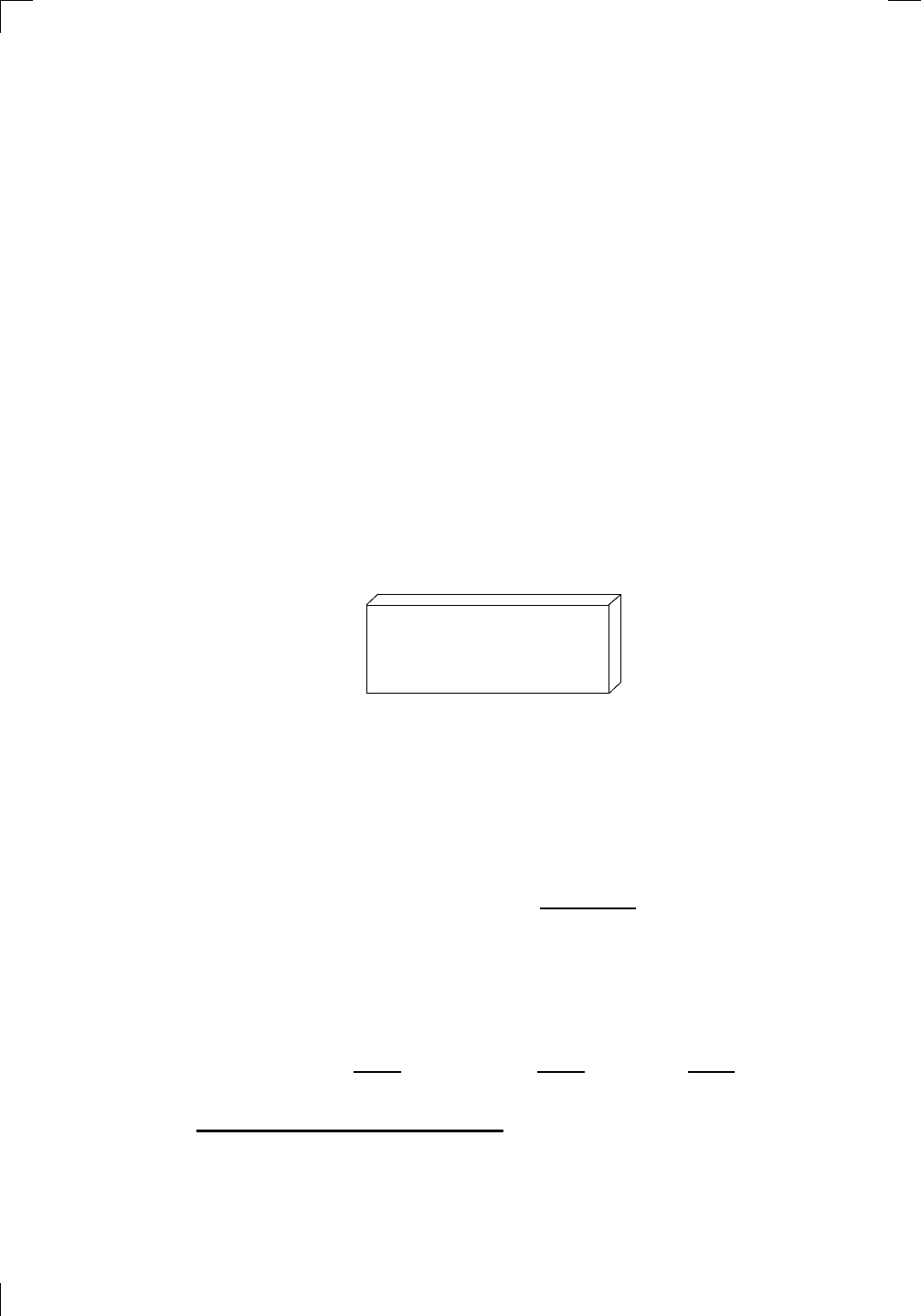
Section 29.1.2: The shell method • 621
This weird solid is a pretty lumpy bagel half, but its volume is fairly close to
what we’re looking for. The thinner the maximum shell thickness, the better
the approximation. As before, integrating takes care of both the addition of
all the shell volumes and also taking the limit as the maximum shell thickness
goes to zero.
First we need to find the volume of one generic shell. The easiest way to
do this is to think of the shell as a really thin metal can without a top or
bottom. As you can see from the picture of the shell on the previous page,
the height of the can is y units, the radius is x units, and the thickness is dx
units. Imagine cutting the can down the side with some sharp scissors, then
unfolding it and flattening it out into a thin rectangle-like piece of metal. It’s
not actually a rectangle, of course. You see, a rectangle is a 2-dimensional
object, whereas the unrolled can is 3-dimensional—although the can is pretty
thin, it still has some thickness. (Even a piece of paper has some thickness,
or else a ream of paper would be really really thin.) Now it’s actually not
even a rectangular prism, since the inner radius of the can isn’t exactly the
same as the outer radius. But the point is, it’s almost a rectangular prism.
The thinner the can gets, the closer it is to a rectangular prism, and when we
take limits in the end (using the integral), everything will work out.
∗
So, the
idealized version of the unfolded can looks like this:
PSfrag
replacements
(
a, b)
[
a, b]
(
a, b]
[
a, b)
(
a, ∞)
[
a, ∞)
(
−∞, b)
(
−∞, b]
(
−∞, ∞)
{
x : a < x < b}
{
x : a ≤ x ≤ b}
{
x : a < x ≤ b}
{
x : a ≤ x < b}
{
x : x ≥ a}
{
x : x > a}
{
x : x ≤ b}
{
x : x < b}
R
a
b
shado
w
0
1
4
−
2
3
−
3
g(
x) = x
2
f(
x) = x
3
g(
x) = x
2
f(
x) = x
3
mirror
(y = x)
f
−
1
(x) =
3
√
x
y = h
(x)
y = h
−
1
(x)
y =
(x − 1)
2
−
1
x
Same
height
−
x
Same
length,
opp
osite signs
y = −
2x
−
2
1
y =
1
2
x − 1
2
−
1
y =
2
x
y =
10
x
y =
2
−x
y =
log
2
(x)
4
3
units
mirror
(x-axis)
y = |
x|
y = |
log
2
(x)|
θ radians
θ units
30
◦
=
π
6
45
◦
=
π
4
60
◦
=
π
3
120
◦
=
2
π
3
135
◦
=
3
π
4
150
◦
=
5
π
6
90
◦
=
π
2
180
◦
= π
210
◦
=
7
π
6
225
◦
=
5
π
4
240
◦
=
4
π
3
270
◦
=
3
π
2
300
◦
=
5
π
3
315
◦
=
7
π
4
330
◦
=
11
π
6
0
◦
=
0 radians
θ
hyp
otenuse
opp
osite
adjacen
t
0
(≡ 2π)
π
2
π
3
π
2
I
I
I
I
II
IV
θ
(
x, y)
x
y
r
7
π
6
reference
angle
reference
angle =
π
6
sin
+
sin −
cos
+
cos −
tan
+
tan −
A
S
T
C
7
π
4
9
π
13
5
π
6
(this
angle is
5π
6
clo
ckwise)
1
2
1
2
3
4
5
6
0
−
1
−
2
−
3
−
4
−
5
−
6
−
3π
−
5
π
2
−
2π
−
3
π
2
−
π
−
π
2
3
π
3
π
5
π
2
2
π
3
π
2
π
π
2
y =
sin(x)
1
0
−
1
−
3π
−
5
π
2
−
2π
−
3
π
2
−
π
−
π
2
3
π
5
π
2
2
π
2
π
3
π
2
π
π
2
y =
sin(x)
y =
cos(x)
−
π
2
π
2
y =
tan(x), −
π
2
<
x <
π
2
0
−
π
2
π
2
y =
tan(x)
−
2π
−
3π
−
5
π
2
−
3
π
2
−
π
−
π
2
π
2
3
π
3
π
5
π
2
2
π
3
π
2
π
y =
sec(x)
y =
csc(x)
y =
cot(x)
y = f (
x)
−
1
1
2
y = g(
x)
3
y = h
(x)
4
5
−
2
f(
x) =
1
x
g(
x) =
1
x
2
etc.
0
1
π
1
2
π
1
3
π
1
4
π
1
5
π
1
6
π
1
7
π
g(
x) = sin
1
x
1
0
−
1
L
10
100
200
y =
π
2
y = −
π
2
y =
tan
−1
(x)
π
2
π
y =
sin(
x)
x
,
x > 3
0
1
−
1
a
L
f(
x) = x sin (1/x)
(0 <
x < 0.3)
h
(x) = x
g(
x) = −x
a
L
lim
x
→a
+
f(x) = L
lim
x
→a
+
f(x) = ∞
lim
x
→a
+
f(x) = −∞
lim
x
→a
+
f(x) DNE
lim
x
→a
−
f(x) = L
lim
x
→a
−
f(x) = ∞
lim
x
→a
−
f(x) = −∞
lim
x
→a
−
f(x) DNE
M
}
lim
x
→a
−
f(x) = M
lim
x
→a
f(x) = L
lim
x
→a
f(x) DNE
lim
x
→∞
f(x) = L
lim
x
→∞
f(x) = ∞
lim
x
→∞
f(x) = −∞
lim
x
→∞
f(x) DNE
lim
x
→−∞
f(x) = L
lim
x
→−∞
f(x) = ∞
lim
x
→−∞
f(x) = −∞
lim
x
→−∞
f(x) DNE
lim
x →a
+
f(
x) = ∞
lim
x →a
+
f(
x) = −∞
lim
x →a
−
f(
x) = ∞
lim
x →a
−
f(
x) = −∞
lim
x →a
f(
x) = ∞
lim
x →a
f(
x) = −∞
lim
x →a
f(
x) DNE
y = f (
x)
a
y =
|
x|
x
1
−
1
y =
|
x + 2|
x +
2
1
−
1
−
2
1
2
3
4
a
a
b
y = x sin
1
x
y = x
y = −
x
a
b
c
d
C
a
b
c
d
−
1
0
1
2
3
time
y
t
u
(
t, f(t))
(
u, f(u))
time
y
t
u
y
x
(
x, f(x))
y = |
x|
(
z, f(z))
z
y = f (
x)
a
tangen
t at x = a
b
tangen
t at x = b
c
tangen
t at x = c
y = x
2
tangen
t
at x = −
1
u
v
uv
u +
∆u
v +
∆v
(
u + ∆u)(v + ∆v)
∆
u
∆
v
u
∆v
v∆
u
∆
u∆v
y = f (
x)
1
2
−
2
y = |
x
2
− 4|
y = x
2
− 4
y = −
2x + 5
y = g(
x)
1
2
3
4
5
6
7
8
9
0
−
1
−
2
−
3
−
4
−
5
−
6
y = f (
x)
3
−
3
3
−
3
0
−
1
2
easy
hard
flat
y = f
0
(
x)
3
−
3
0
−
1
2
1
−
1
y =
sin(x)
y = x
x
A
B
O
1
C
D
sin(
x)
tan(
x)
y =
sin
(x)
x
π
2
π
1
−
1
x =
0
a =
0
x
> 0
a
> 0
x
< 0
a
< 0
rest
position
+
−
y = x
2
sin
1
x
N
A
B
H
a
b
c
O
H
A
B
C
D
h
r
R
θ
1000
2000
α
β
p
h
y = g(
x) = log
b
(x)
y = f(
x) = b
x
y = e
x
5
10
1
2
3
4
0
−
1
−
2
−
3
−
4
y =
ln(x)
y =
cosh(x)
y =
sinh(x)
y =
tanh(x)
y =
sech(x)
y =
csch(x)
y =
coth(x)
1
−
1
y = f (
x)
original
function
in
verse function
slop
e = 0 at (x, y)
slop
e is infinite at (y, x)
−
108
2
5
1
2
1
2
3
4
5
6
0
−
1
−
2
−
3
−
4
−
5
−
6
−
3π
−
5
π
2
−
2π
−
3
π
2
−
π
−
π
2
3
π
3
π
5
π
2
2
π
3
π
2
π
π
2
y =
sin(x)
1
0
−
1
−
3π
−
5
π
2
−
2π
−
3
π
2
−
π
−
π
2
3
π
5
π
2
2
π
2
π
3
π
2
π
π
2
y =
sin(x)
y =
sin(x), −
π
2
≤ x ≤
π
2
−
2
−
1
0
2
π
2
−
π
2
y =
sin
−1
(x)
y =
cos(x)
π
π
2
y =
cos
−1
(x)
−
π
2
1
x
α
β
y =
tan(x)
y =
tan(x)
1
y =
tan
−1
(x)
y =
sec(x)
y =
sec
−1
(x)
y =
csc
−1
(x)
y =
cot
−1
(x)
1
y =
cosh
−1
(x)
y =
sinh
−1
(x)
y =
tanh
−1
(x)
y =
sech
−1
(x)
y =
csch
−1
(x)
y =
coth
−1
(x)
(0
, 3)
(2
, −1)
(5
, 2)
(7
, 0)
(
−1, 44)
(0
, 1)
(1
, −12)
(2
, 305)
y =
1
2
(2
, 3)
y = f (
x)
y = g(
x)
a
b
c
a
b
c
s
c
0
c
1
(
a, f(a))
(
b, f(b))
1
2
1
2
3
4
5
6
0
−
1
−
2
−
3
−
4
−
5
−
6
−
3π
−
5
π
2
−
2π
−
3
π
2
−
π
−
π
2
3
π
3
π
5
π
2
2
π
3
π
2
π
π
2
y =
sin(x)
1
0
−
1
−
3π
−
5
π
2
−
2π
−
3
π
2
−
π
−
π
2
3
π
5
π
2
2
π
2
π
3
π
2
π
π
2
c
OR
Lo
cal maximum
Lo
cal minimum
Horizon
tal point of inflection
1
e
y = f
0
(
x)
y = f(
x) = x ln(x)
−
1
e
?
y = f(
x) = x
3
y = g(
x) = x
4
x
f(
x)
−
3
−
2
−
1
0
1
2
1
2
3
4
+
−
?
1
5
6
3
f
0
(
x)
2 −
1
2
√
6
2
+
1
2
√
6
f
00
(
x)
7
8
g
00
(
x)
f
00
(
x)
0
y =
(
x − 3)(x − 1)
2
x
3
(
x + 2)
y = x ln
(x)
1
e
−
1
e
5
−
108
2
α
β
2 −
1
2
√
6
2
+
1
2
√
6
y = x
2
(
x − 5)
3
−
e
−
1/2
√
3
e
−
1/2
√
3
−
e
−3/2
e
−
3/2
−
1
√
3
1
√
3
−
1
1
y = xe
−
3x
2
/2
y =
x
3
− 6
x
2
+ 13x − 8
x
28
2
600
500
400
300
200
100
0
−
100
−
200
−
300
−
400
−
500
−
600
0
10
−
10
5
−
5
20
−
20
15
−
15
0
4
5
6
x
P
0
(
x)
+
−
−
existing
fence
new
fence
enclosure
A
h
b
H
99
100
101
h
dA/dh
r
h
1
2
7
shallo
w
deep
LAND
SEA
N
y
z
s
t
3
11
9
L
(11)
√
11
y = L
(x)
y = f (
x)
11
y = L
(x)
y = f (
x)
F
P
a
a +
∆x
f(
a + ∆x)
L
(a + ∆x)
f(
a)
error
d
f
∆
x
a
b
y = f (
x)
true
zero
starting
approximation
b
etter approximation
v
t
3
5
50
40
60
4
20
30
25
t
1
t
2
t
3
t
4
t
n
−2
t
n
−1
t
0
= a
t
n
= b
v
1
v
2
v
3
v
4
v
n
−1
v
n
−
30
6
30
|
v|
a
b
p
q
c
v(
c)
v(
c
1
)
v(
c
2
)
v(
c
3
)
v(
c
4
)
v(
c
5
)
v(
c
6
)
t
1
t
2
t
3
t
4
t
5
c
1
c
2
c
3
c
4
c
5
c
6
t
0
=
a
t
6
=
b
t
16
=
b
t
10
=
b
a
b
x
y
y = f (
x)
1
2
y = x
5
0
−
2
y =
1
a
b
y =
sin(x)
π
−
π
0
−
1
−
2
0
2
4
y = x
2
0
1
2
3
4
2
n
4
n
6
n
2(
n−2)
n
2(
n−1)
n
2
n
n
=
2
width
of each interval =
2
n
−
2
1
3
0
I
I
I
I
II
IV
4
y
dx
y = −
x
2
− 2x + 3
3
−
5
y = |−
x
2
− 2x + 3|
I
I
I
I
Ia
5
3
0
1
2
a
b
y = f (
x)
y = g(
x)
y = x
2
a
b
5
3
0
1
2
y =
√
x
2
√
2
2
2
dy
x
2
a
b
y = f (
x)
y = g(
x)
M
m
1
2
−
1
−
2
0
y = e
−
x
2
1
2
e
−
1/4
f
a
v
y = f
a
v
c
A
M
0
1
2
a
b
x
t
y = f(
t)
F (
x )
y = f(
t)
F (
x + h )
x + h
F (
x + h) − F (x)
f(
x)
1
2
y =
sin(x)
π
−
π
−
1
−
2
y =
1
x
y = x
2
1
2
1
−
1
y =
ln|x|
θ
a
x
a
x
p
a
2
− x
2
3
x
p
9 − x
2
p
x
2
+ a
2
x
a
p
x
2
+ 15
x
√
15
x
p
x
2
− a
2
a
x
p
x
2
− 4
2
x
−
p
x
2
− a
2
a
x
−
p
x
2
− 4
2
y = f (
x)
a
b
a + ε
ε
Z
b
a
+ε
f(x) dx
small
ev
en smaller
y = g(
x)
infinite
area
finite
area
1
y =
1
x
y =
1
x
p
, p
< 1 (typical)
y =
1
x
p
, p
> 1 (typical)
a
1
a
2
a
3
a
4
a
5
a
6
a
7
a
8
1
2
3
4
5
6
7
8
n
a
n
x
y
y = f (
x)
(
a, f(a))
a
−
1
0
1
a
6
1
2
7
1
2
7
?
−
2
−
1
−
2
t =
0
t = π
/6
t = π
/4
t = π
/3
t = π
/2
3
0
t = −
2
t = −
3/2
t = ±
1
t = −
1/2
t =
0
t =
1/2
t =
3/2
t =
2
12
−
12
θ
r
P
θ
r
P
11
π
6
2
(
−1, −1)
wrong
point
π
4
5
π
4
√
2
(0
, 1)
(0
, −3)
(
−2, 0)
π
2
3
π
2
π
r =
3 sin(θ)
3
π
2
θ
2
π
1
0
−
1
−
2
−
3
0
3
2
−
3
2
0
r =
1 + 2 cos(θ)
2
π
3
4
π
3
0
π
0
pi
−
3
2
3
π
2
1
2
3
0
−
1
−
2
−
3
0 ≤ θ ≤
2
π
3
0 ≤ θ ≤ π
0 ≤ θ ≤ 2
π
r =
1 + cos(θ)
r =
1 +
3
4
cos(
θ)
−
1
4
r =
sin(2θ)
r = sin(3θ)
r =
1
π
θ
0 ≤ θ ≤ 4π
r =
2
1 + sin(θ)
−
π
4
≤ θ ≤
5π
4
0 ≤ θ ≤ 2π
0 ≤ θ ≤ π
−4
−5
4
5
f(θ)
f(θ + dθ)
θ
dθ
θ + dθ
approximating region
exact region
0 ≤ θ ≤ 2π
r = |1 + 2 cos(θ)|
2i
2 − 3i
−1
θ = 0
θ =
π
4
θ =
π
2
θ =
2π
3
θ = π
θ =
13π
12
θ =
3π
2
θ =
7π
4
1 = e
0
e
i
π
4
i = e
i
π
2
e
i
2π
3
−1 = e
iπ
e
i
13π
12
−i = e
i
3π
2
e
i
7π
4
i
−i
1
θ
1 − i
2i
−2i
2
−2
6i
−6i
6
−6
−
√
3
R
ϕ
2
1/5
θ =
π
6
θ =
17π
30
θ =
29π
30
θ =
41π
30
θ =
53π
30
z
0
z
1
z
2
z
3
z
4
−
√
3
2
√
3
2
1
2
i
−i
19π
6
−i
7π
6
i
5π
6
i
17π
6
i
29π
6
ln(2)
−
7π
4
−
3π
4
π
4
5π
4
9π
4
3
2
i
0
1
2
3
4
dx
y
x
y =
p
1 − (x − 3)
2
2πx
The thickness is dx units, and the side we cut along is still the height of the
cylindrical shell, that is, y units. How about the long side? Well, that is equal
to the circumference of the shell (think about it!) which is 2πx units, since
the radius of the shell is basically x units. So, the volume of the shell is very
close to 2πxy dx cubic units. Now all we have to do is integrate from x = 2
to x = 4 to see that the volume of the bagel half (in cubic units) is
Z
4
2
2πxy dx = 2π
Z
4
2
x
p
1 − (x − 3)
2
dx.
Great—we’ve now reduced the problem to evaluating a definite integral, but
it’s a bit of a messy one. Start off by substituting t = x −3, so dt = dx; also,
when x = 2, we have t = −1, and when x = 4, we see that t = 1. So in t-land,
the integral becomes
2π
Z
1
−1
(t + 3)
p
1 − t
2
dt = 2π
Z
1
−1
t
p
1 − t
2
dt + 3
Z
1
−1
p
1 − t
2
dt
.
∗
More formally, we can view the volume of the shell as the difference in volumes of
the outer shell (of radius x + dx units) and the inner shell (of radius x units). Both shells
have height y units, so the volume of the shell is πy((x + dx)
2
− x
2
), which simplifies to
2πxy dx + πy(dx)
2
cubic units. When this is integrated, the second term vanishes due to
the negligible quantity (dx)
2
.
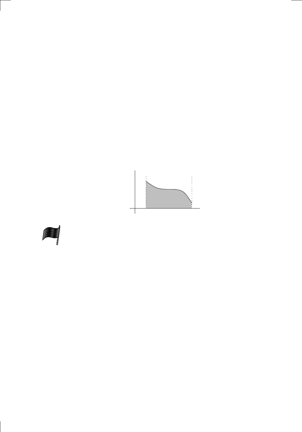
622 • Volumes, Arc Lengths, and Surface Areas
The first integral could be done by substituting u = 1 − t
2
, and the second
could be done by a trig substitution. A better way to do them is to note that
the first integral is actually equal to 0, since the integrand is an odd function
of t and the region of integration [−1, 1] is symmetric about t = 0. (We proved
this shortcut at the end of Section 18.1.1 of Chapter 18.) Furthermore, the
easiest way to do the second integral (ignoring the factor of 3 out front for the
moment) is to realize that it’s equal to the area in square units of a semicircle
of radius 1 unit, which is π/2. So without too much work, we see that the total
answer is 3π
2
, therefore the volume of the bagel half is 3π
2
cubic units. The
method we just used is, unsurprisingly, called the shell method (also known
as the method of cylindrical shells).
29.1.3 Summary . . . and variations
So far we have seen how to use the disc and shell methods in the special
case of our semicircle. The same method works for general regions which are
contained between a curve, the x-axis, and two vertical lines:
PSfrag
replacements
(
a, b)
[
a, b]
(
a, b]
[
a, b)
(
a, ∞)
[
a, ∞)
(
−∞, b)
(
−∞, b]
(
−∞, ∞)
{
x : a < x < b}
{
x : a ≤ x ≤ b}
{
x : a < x ≤ b}
{
x : a ≤ x < b}
{
x : x ≥ a}
{
x : x > a}
{
x : x ≤ b}
{
x : x < b}
R
a
b
shado
w
0
1
4
−
2
3
−
3
g(
x) = x
2
f(
x) = x
3
g(
x) = x
2
f(
x) = x
3
mirror
(y = x)
f
−
1
(x) =
3
√
x
y = h
(x)
y = h
−
1
(x)
y =
(x − 1)
2
−
1
x
Same
height
−
x
Same
length,
opp
osite signs
y = −
2x
−
2
1
y =
1
2
x − 1
2
−
1
y =
2
x
y =
10
x
y =
2
−x
y =
log
2
(x)
4
3
units
mirror
(x-axis)
y = |
x|
y = |
log
2
(x)|
θ radians
θ units
30
◦
=
π
6
45
◦
=
π
4
60
◦
=
π
3
120
◦
=
2
π
3
135
◦
=
3
π
4
150
◦
=
5
π
6
90
◦
=
π
2
180
◦
= π
210
◦
=
7
π
6
225
◦
=
5
π
4
240
◦
=
4
π
3
270
◦
=
3
π
2
300
◦
=
5
π
3
315
◦
=
7
π
4
330
◦
=
11
π
6
0
◦
=
0 radians
θ
hyp
otenuse
opp
osite
adjacen
t
0
(≡ 2π)
π
2
π
3
π
2
I
I
I
I
II
IV
θ
(
x, y)
x
y
r
7
π
6
reference
angle
reference
angle =
π
6
sin
+
sin −
cos
+
cos −
tan
+
tan −
A
S
T
C
7
π
4
9
π
13
5
π
6
(this
angle is
5π
6
clo
ckwise)
1
2
1
2
3
4
5
6
0
−
1
−
2
−
3
−
4
−
5
−
6
−
3π
−
5
π
2
−
2π
−
3
π
2
−
π
−
π
2
3
π
3
π
5
π
2
2
π
3
π
2
π
π
2
y =
sin(x)
1
0
−
1
−
3π
−
5
π
2
−
2π
−
3
π
2
−
π
−
π
2
3
π
5
π
2
2
π
2
π
3
π
2
π
π
2
y =
sin(x)
y =
cos(x)
−
π
2
π
2
y =
tan(x), −
π
2
<
x <
π
2
0
−
π
2
π
2
y =
tan(x)
−
2π
−
3π
−
5
π
2
−
3
π
2
−
π
−
π
2
π
2
3
π
3
π
5
π
2
2
π
3
π
2
π
y =
sec(x)
y =
csc(x)
y =
cot(x)
y = f(
x)
−
1
1
2
y = g(
x)
3
y = h
(x)
4
5
−
2
f(
x) =
1
x
g(
x) =
1
x
2
etc.
0
1
π
1
2
π
1
3
π
1
4
π
1
5
π
1
6
π
1
7
π
g(
x) = sin
1
x
1
0
−
1
L
10
100
200
y =
π
2
y = −
π
2
y =
tan
−1
(x)
π
2
π
y =
sin(
x)
x
,
x > 3
0
1
−
1
a
L
f(
x) = x sin (1/x)
(0 <
x < 0.3)
h
(x) = x
g(
x) = −x
a
L
lim
x
→a
+
f(x) = L
lim
x
→a
+
f(x) = ∞
lim
x
→a
+
f(x) = −∞
lim
x
→a
+
f(x) DNE
lim
x
→a
−
f(x) = L
lim
x
→a
−
f(x) = ∞
lim
x
→a
−
f(x) = −∞
lim
x
→a
−
f(x) DNE
M
}
lim
x
→a
−
f(x) = M
lim
x
→a
f(x) = L
lim
x
→a
f(x) DNE
lim
x
→∞
f(x) = L
lim
x
→∞
f(x) = ∞
lim
x
→∞
f(x) = −∞
lim
x
→∞
f(x) DNE
lim
x
→−∞
f(x) = L
lim
x
→−∞
f(x) = ∞
lim
x
→−∞
f(x) = −∞
lim
x
→−∞
f(x) DNE
lim
x →a
+
f(
x) = ∞
lim
x →a
+
f(
x) = −∞
lim
x →a
−
f(
x) = ∞
lim
x →a
−
f(
x) = −∞
lim
x →a
f(
x) = ∞
lim
x →a
f(
x) = −∞
lim
x →a
f(
x) DNE
y = f(
x)
a
y =
|
x|
x
1
−
1
y =
|
x + 2|
x +
2
1
−
1
−
2
1
2
3
4
a
a
b
y = x sin
1
x
y = x
y = −
x
a
b
c
d
C
a
b
c
d
−
1
0
1
2
3
time
y
t
u
(
t, f(t))
(
u, f(u))
time
y
t
u
y
x
(
x, f(x))
y = |
x|
(
z, f(z))
z
y = f(
x)
a
tangen
t at x = a
b
tangen
t at x = b
c
tangen
t at x = c
y = x
2
tangen
t
at x = −
1
u
v
uv
u +
∆u
v +
∆v
(
u + ∆u)(v + ∆v)
∆
u
∆
v
u
∆v
v∆
u
∆
u∆v
y = f(
x)
1
2
−
2
y = |
x
2
− 4|
y = x
2
− 4
y = −
2x + 5
y = g(
x)
1
2
3
4
5
6
7
8
9
0
−
1
−
2
−
3
−
4
−
5
−
6
y = f(
x)
3
−
3
3
−
3
0
−
1
2
easy
hard
flat
y = f
0
(
x)
3
−
3
0
−
1
2
1
−
1
y =
sin(x)
y = x
x
A
B
O
1
C
D
sin
(x)
tan
(x)
y =
sin
(x)
x
π
2
π
1
−
1
x =
0
a =
0
x
> 0
a
> 0
x
< 0
a
< 0
rest
position
+
−
y = x
2
sin
1
x
N
A
B
H
a
b
c
O
H
A
B
C
D
h
r
R
θ
1000
2000
α
β
p
h
y = g(
x) = log
b
(x)
y = f(
x) = b
x
y = e
x
5
10
1
2
3
4
0
−
1
−
2
−
3
−
4
y =
ln(x)
y =
cosh(x)
y =
sinh(x)
y =
tanh(x)
y =
sech(x)
y =
csch(x)
y =
coth(x)
1
−
1
y = f(
x)
original
function
in
verse function
slop
e = 0 at (x, y)
slop
e is infinite at (y, x)
−
108
2
5
1
2
1
2
3
4
5
6
0
−
1
−
2
−
3
−
4
−
5
−
6
−
3π
−
5
π
2
−
2π
−
3
π
2
−
π
−
π
2
3
π
3
π
5
π
2
2
π
3
π
2
π
π
2
y =
sin(x)
1
0
−
1
−
3π
−
5
π
2
−
2π
−
3
π
2
−
π
−
π
2
3
π
5
π
2
2
π
2
π
3
π
2
π
π
2
y =
sin(x)
y =
sin(x), −
π
2
≤ x ≤
π
2
−
2
−
1
0
2
π
2
−
π
2
y =
sin
−1
(x)
y =
cos(x)
π
π
2
y =
cos
−1
(x)
−
π
2
1
x
α
β
y =
tan(x)
y =
tan(x)
1
y =
tan
−1
(x)
y =
sec(x)
y =
sec
−1
(x)
y =
csc
−1
(x)
y =
cot
−1
(x)
1
y =
cosh
−1
(x)
y =
sinh
−1
(x)
y =
tanh
−1
(x)
y =
sech
−1
(x)
y =
csch
−1
(x)
y =
coth
−1
(x)
(0
, 3)
(2
, −1)
(5
, 2)
(7
, 0)
(
−1, 44)
(0
, 1)
(1
, −12)
(2
, 305)
y =
1
2
(2
, 3)
y = f(
x)
y = g(
x)
a
b
c
a
b
c
s
c
0
c
1
(
a, f(a))
(
b, f(b))
1
2
1
2
3
4
5
6
0
−
1
−
2
−
3
−
4
−
5
−
6
−
3π
−
5
π
2
−
2π
−
3
π
2
−
π
−
π
2
3
π
3
π
5
π
2
2
π
3
π
2
π
π
2
y =
sin(x)
1
0
−
1
−
3π
−
5
π
2
−
2π
−
3
π
2
−
π
−
π
2
3
π
5
π
2
2
π
2
π
3
π
2
π
π
2
c
OR
Lo
cal maximum
Lo
cal minimum
Horizon
tal point of inflection
1
e
y = f
0
(
x)
y = f (
x) = x ln(x)
−
1
e
?
y = f (
x) = x
3
y = g(
x) = x
4
x
f(
x)
−
3
−
2
−
1
0
1
2
1
2
3
4
+
−
?
1
5
6
3
f
0
(
x)
2 −
1
2
√
6
2
+
1
2
√
6
f
00
(
x)
7
8
g
00
(
x)
f
00
(
x)
0
y =
(
x − 3)(x − 1)
2
x
3
(
x + 2)
y = x ln(
x)
1
e
−
1
e
5
−
108
2
α
β
2 −
1
2
√
6
2
+
1
2
√
6
y = x
2
(
x − 5)
3
−
e
−
1/2
√
3
e
−
1/2
√
3
−
e
−3/2
e
−
3/2
−
1
√
3
1
√
3
−
1
1
y = xe
−
3x
2
/2
y =
x
3
− 6
x
2
+ 13x − 8
x
28
2
600
500
400
300
200
100
0
−
100
−
200
−
300
−
400
−
500
−
600
0
10
−
10
5
−
5
20
−
20
15
−
15
0
4
5
6
x
P
0
(
x)
+
−
−
existing
fence
new
fence
enclosure
A
h
b
H
99
100
101
h
dA/dh
r
h
1
2
7
shallo
w
deep
LAND
SEA
N
y
z
s
t
3
11
9
L
(11)
√
11
y = L
(x)
y = f(
x)
11
y = L
(x)
y = f(
x)
F
P
a
a +
∆x
f(
a + ∆x)
L
(a + ∆x)
f(
a)
error
d
f
∆
x
a
b
y = f(
x)
true
zero
starting
approximation
b
etter approximation
v
t
3
5
50
40
60
4
20
30
25
t
1
t
2
t
3
t
4
t
n
−2
t
n
−1
t
0
= a
t
n
= b
v
1
v
2
v
3
v
4
v
n
−1
v
n
−
30
6
30
|
v|
a
b
p
q
c
v(
c)
v(
c
1
)
v(
c
2
)
v(
c
3
)
v(
c
4
)
v(
c
5
)
v(
c
6
)
t
1
t
2
t
3
t
4
t
5
c
1
c
2
c
3
c
4
c
5
c
6
t
0
=
a
t
6
=
b
t
16
=
b
t
10
=
b
a
b
x
y
y = f(
x)
1
2
y = x
5
0
−
2
y =
1
a
b
y =
sin(x)
π
−
π
0
−
1
−
2
0
2
4
y = x
2
0
1
2
3
4
2
n
4
n
6
n
2(
n−2)
n
2(
n−1)
n
2
n
n
=
2
width
of each interval =
2
n
−
2
1
3
0
I
I
I
I
II
IV
4
y
dx
y = −
x
2
− 2x + 3
3
−
5
y = |−
x
2
− 2x + 3|
I
I
I
I
Ia
5
3
0
1
2
a
b
y = f (
x)
y = g(
x)
y = x
2
a
b
5
3
0
1
2
y =
√
x
2
√
2
2
2
dy
x
2
a
b
y = f(
x)
y = g(
x)
M
m
1
2
−
1
−
2
0
y = e
−
x
2
1
2
e
−
1/4
f
a
v
y = f
a
v
c
A
M
0
1
2
a
b
x
t
y = f (
t)
F (
x )
y = f (
t)
F (
x + h )
x + h
F (
x + h) − F (x)
f(
x)
1
2
y =
sin(x)
π
−
π
−
1
−
2
y =
1
x
y = x
2
1
2
1
−
1
y =
ln|x|
θ
a
x
a
x
p
a
2
− x
2
3
x
p
9 − x
2
p
x
2
+ a
2
x
a
p
x
2
+ 15
x
√
15
x
p
x
2
− a
2
a
x
p
x
2
− 4
2
x
−
p
x
2
− a
2
a
x
−
p
x
2
− 4
2
y = f(
x)
a
b
a + ε
ε
Z
b
a
+ε
f(x) dx
small
ev
en smaller
y = g(
x)
infinite
area
finite
area
1
y =
1
x
y =
1
x
p
, p
< 1 (typical)
y =
1
x
p
, p
> 1 (typical)
a
1
a
2
a
3
a
4
a
5
a
6
a
7
a
8
1
2
3
4
5
6
7
8
n
a
n
x
y
y = f(
x)
(
a, f(a))
a
−
1
0
1
a
6
1
2
7
1
2
7
?
−
2
−
1
−
2
t =
0
t = π
/6
t = π
/4
t = π
/3
t = π
/2
3
0
t = −
2
t = −
3/2
t = ±
1
t = −
1/2
t =
0
t =
1/2
t =
3/2
t =
2
12
−
12
θ
r
P
θ
r
P
11
π
6
2
(
−1, −1)
wrong
point
π
4
5
π
4
√
2
(0
, 1)
(0
, −3)
(
−2, 0)
π
2
3
π
2
π
r =
3 sin(θ)
3
π
2
θ
2
π
1
0
−
1
−
2
−
3
0
3
2
−
3
2
0
r =
1 + 2 cos(θ)
2
π
3
4
π
3
0
π
0
pi
−
3
2
3
π
2
1
2
3
0
−
1
−
2
−
3
0 ≤ θ ≤
2
π
3
0 ≤ θ ≤ π
0 ≤ θ ≤ 2
π
r =
1 + cos(θ)
r =
1 +
3
4
cos(
θ)
−
1
4
r =
sin(2θ)
r =
sin(3θ)
r =
1
π
θ
0 ≤ θ ≤ 4
π
r =
2
1 + sin(θ)
−
π
4
≤ θ ≤
5π
4
0 ≤ θ ≤ 2π
0 ≤ θ ≤ π
−4
−5
4
5
f(θ)
f(θ + dθ)
θ
dθ
θ + dθ
approximating region
exact region
0 ≤ θ ≤ 2π
r = |1 + 2 cos(θ)|
2i
2 − 3i
−1
θ = 0
θ =
π
4
θ =
π
2
θ =
2π
3
θ = π
θ =
13π
12
θ =
3π
2
θ =
7π
4
1 = e
0
e
i
π
4
i = e
i
π
2
e
i
2π
3
−1 = e
iπ
e
i
13π
12
−i = e
i
3π
2
e
i
7π
4
i
−i
1
θ
1 − i
2i
−2i
2
−2
6i
−6i
6
−6
−
√
3
R
ϕ
2
1/5
θ =
π
6
θ =
17π
30
θ =
29π
30
θ =
41π
30
θ =
53π
30
z
0
z
1
z
2
z
3
z
4
−
√
3
2
√
3
2
1
2
i
−i
19π
6
−i
7π
6
i
5π
6
i
17π
6
i
29π
6
ln(2)
−
7π
4
−
3π
4
π
4
5π
4
9π
4
3
2
i
0
1
2
3
4
dx
y
x
y =
p
1 − (x − 3)
2
2πx
a
b
y = f(x)
By the same reasoning that we used above in the special case of the semicircle,
we can arrive at the following principles:
PSfrag
replacements
(
a, b)
[
a, b]
(
a, b]
[
a, b)
(
a, ∞)
[
a, ∞)
(
−∞, b)
(
−∞, b]
(
−∞, ∞)
{
x : a < x < b}
{
x : a ≤ x ≤ b}
{
x : a < x ≤ b}
{
x : a ≤ x < b}
{
x : x ≥ a}
{
x : x > a}
{
x : x ≤ b}
{
x : x < b}
R
a
b
shado
w
0
1
4
−
2
3
−
3
g(
x) = x
2
f(
x) = x
3
g(
x) = x
2
f(
x) = x
3
mirror
(y = x)
f
−
1
(x) =
3
√
x
y = h
(x)
y = h
−
1
(x)
y =
(x − 1)
2
−
1
x
Same
height
−
x
Same
length,
opp
osite signs
y = −
2x
−
2
1
y =
1
2
x − 1
2
−
1
y =
2
x
y =
10
x
y =
2
−x
y =
log
2
(x)
4
3
units
mirror
(x-axis)
y = |
x|
y = |
log
2
(x)|
θ radians
θ units
30
◦
=
π
6
45
◦
=
π
4
60
◦
=
π
3
120
◦
=
2
π
3
135
◦
=
3
π
4
150
◦
=
5
π
6
90
◦
=
π
2
180
◦
= π
210
◦
=
7
π
6
225
◦
=
5
π
4
240
◦
=
4
π
3
270
◦
=
3
π
2
300
◦
=
5
π
3
315
◦
=
7
π
4
330
◦
=
11
π
6
0
◦
=
0 radians
θ
hyp
otenuse
opp
osite
adjacen
t
0
(≡ 2π)
π
2
π
3
π
2
I
I
I
I
II
IV
θ
(
x, y)
x
y
r
7
π
6
reference
angle
reference
angle =
π
6
sin
+
sin −
cos
+
cos −
tan
+
tan −
A
S
T
C
7
π
4
9
π
13
5
π
6
(this
angle is
5π
6
clo
ckwise)
1
2
1
2
3
4
5
6
0
−
1
−
2
−
3
−
4
−
5
−
6
−
3π
−
5
π
2
−
2π
−
3
π
2
−
π
−
π
2
3
π
3
π
5
π
2
2
π
3
π
2
π
π
2
y =
sin(x)
1
0
−
1
−
3π
−
5
π
2
−
2π
−
3
π
2
−
π
−
π
2
3
π
5
π
2
2
π
2
π
3
π
2
π
π
2
y =
sin(x)
y =
cos(x)
−
π
2
π
2
y =
tan(x), −
π
2
<
x <
π
2
0
−
π
2
π
2
y =
tan(x)
−
2π
−
3π
−
5
π
2
−
3
π
2
−
π
−
π
2
π
2
3
π
3
π
5
π
2
2
π
3
π
2
π
y =
sec(x)
y =
csc(x)
y =
cot(x)
y = f (
x)
−
1
1
2
y = g(
x)
3
y = h
(x)
4
5
−
2
f(
x) =
1
x
g(
x) =
1
x
2
etc.
0
1
π
1
2
π
1
3
π
1
4
π
1
5
π
1
6
π
1
7
π
g(
x) = sin
1
x
1
0
−
1
L
10
100
200
y =
π
2
y = −
π
2
y =
tan
−1
(x)
π
2
π
y =
sin(
x)
x
,
x > 3
0
1
−
1
a
L
f(
x) = x sin (1/x)
(0 <
x < 0.3)
h
(x) = x
g(
x) = −x
a
L
lim
x
→a
+
f(x) = L
lim
x
→a
+
f(x) = ∞
lim
x
→a
+
f(x) = −∞
lim
x
→a
+
f(x) DNE
lim
x
→a
−
f(x) = L
lim
x
→a
−
f(x) = ∞
lim
x
→a
−
f(x) = −∞
lim
x
→a
−
f(x) DNE
M
}
lim
x
→a
−
f(x) = M
lim
x
→a
f(x) = L
lim
x
→a
f(x) DNE
lim
x
→∞
f(x) = L
lim
x
→∞
f(x) = ∞
lim
x
→∞
f(x) = −∞
lim
x
→∞
f(x) DNE
lim
x
→−∞
f(x) = L
lim
x
→−∞
f(x) = ∞
lim
x
→−∞
f(x) = −∞
lim
x
→−∞
f(x) DNE
lim
x →a
+
f(
x) = ∞
lim
x →a
+
f(
x) = −∞
lim
x →a
−
f(
x) = ∞
lim
x →a
−
f(
x) = −∞
lim
x →a
f(
x) = ∞
lim
x →a
f(
x) = −∞
lim
x →a
f(
x) DNE
y = f (
x)
a
y =
|
x|
x
1
−
1
y =
|
x + 2|
x +
2
1
−
1
−
2
1
2
3
4
a
a
b
y = x sin
1
x
y = x
y = −
x
a
b
c
d
C
a
b
c
d
−
1
0
1
2
3
time
y
t
u
(
t, f(t))
(
u, f(u))
time
y
t
u
y
x
(
x, f(x))
y = |
x|
(
z, f(z))
z
y = f (
x)
a
tangen
t at x = a
b
tangen
t at x = b
c
tangen
t at x = c
y = x
2
tangen
t
at x = −
1
u
v
uv
u +
∆u
v +
∆v
(
u + ∆u)(v + ∆v)
∆
u
∆
v
u
∆v
v∆
u
∆
u∆v
y = f (
x)
1
2
−
2
y = |
x
2
− 4|
y = x
2
− 4
y = −
2x + 5
y = g(
x)
1
2
3
4
5
6
7
8
9
0
−
1
−
2
−
3
−
4
−
5
−
6
y = f (
x)
3
−
3
3
−
3
0
−
1
2
easy
hard
flat
y = f
0
(
x)
3
−
3
0
−
1
2
1
−
1
y =
sin(x)
y = x
x
A
B
O
1
C
D
sin(
x)
tan(
x)
y =
sin
(x)
x
π
2
π
1
−
1
x =
0
a =
0
x
> 0
a
> 0
x
< 0
a
< 0
rest
position
+
−
y = x
2
sin
1
x
N
A
B
H
a
b
c
O
H
A
B
C
D
h
r
R
θ
1000
2000
α
β
p
h
y = g(
x) = log
b
(x)
y = f (
x) = b
x
y = e
x
5
10
1
2
3
4
0
−
1
−
2
−
3
−
4
y =
ln(x)
y =
cosh(x)
y =
sinh(x)
y =
tanh(x)
y =
sech(x)
y =
csch(x)
y =
coth(x)
1
−
1
y = f (
x)
original
function
in
verse function
slop
e = 0 at (x, y)
slop
e is infinite at (y, x)
−
108
2
5
1
2
1
2
3
4
5
6
0
−
1
−
2
−
3
−
4
−
5
−
6
−
3π
−
5
π
2
−
2π
−
3
π
2
−
π
−
π
2
3
π
3
π
5
π
2
2
π
3
π
2
π
π
2
y =
sin(x)
1
0
−
1
−
3π
−
5
π
2
−
2π
−
3
π
2
−
π
−
π
2
3
π
5
π
2
2
π
2
π
3
π
2
π
π
2
y =
sin(x)
y =
sin(x), −
π
2
≤ x ≤
π
2
−
2
−
1
0
2
π
2
−
π
2
y =
sin
−1
(x)
y =
cos(x)
π
π
2
y =
cos
−1
(x)
−
π
2
1
x
α
β
y =
tan(x)
y =
tan(x)
1
y =
tan
−1
(x)
y =
sec(x)
y =
sec
−1
(x)
y =
csc
−1
(x)
y =
cot
−1
(x)
1
y =
cosh
−1
(x)
y =
sinh
−1
(x)
y =
tanh
−1
(x)
y =
sech
−1
(x)
y =
csch
−1
(x)
y =
coth
−1
(x)
(0
, 3)
(2
, −1)
(5
, 2)
(7
, 0)
(
−1, 44)
(0
, 1)
(1
, −12)
(2
, 305)
y =
1
2
(2
, 3)
y = f (
x)
y = g(
x)
a
b
c
a
b
c
s
c
0
c
1
(
a, f(a))
(
b, f(b))
1
2
1
2
3
4
5
6
0
−
1
−
2
−
3
−
4
−
5
−
6
−
3π
−
5
π
2
−
2π
−
3
π
2
−
π
−
π
2
3
π
3
π
5
π
2
2
π
3
π
2
π
π
2
y =
sin(x)
1
0
−
1
−
3π
−
5
π
2
−
2π
−
3
π
2
−
π
−
π
2
3
π
5
π
2
2
π
2
π
3
π
2
π
π
2
c
OR
Lo
cal maximum
Lo
cal minimum
Horizon
tal point of inflection
1
e
y = f
0
(
x)
y = f(
x) = x ln(x)
−
1
e
?
y = f(
x) = x
3
y = g(
x) = x
4
x
f(
x)
−
3
−
2
−
1
0
1
2
1
2
3
4
+
−
?
1
5
6
3
f
0
(
x)
2 −
1
2
√
6
2
+
1
2
√
6
f
00
(
x)
7
8
g
00
(
x)
f
00
(
x)
0
y =
(
x − 3)(x − 1)
2
x
3
(
x + 2)
y = x ln
(x)
1
e
−
1
e
5
−
108
2
α
β
2 −
1
2
√
6
2
+
1
2
√
6
y = x
2
(
x − 5)
3
−
e
−
1/2
√
3
e
−
1/2
√
3
−
e
−3/2
e
−
3/2
−
1
√
3
1
√
3
−
1
1
y = xe
−
3x
2
/2
y =
x
3
− 6
x
2
+ 13x − 8
x
28
2
600
500
400
300
200
100
0
−
100
−
200
−
300
−
400
−
500
−
600
0
10
−
10
5
−
5
20
−
20
15
−
15
0
4
5
6
x
P
0
(
x)
+
−
−
existing
fence
new
fence
enclosure
A
h
b
H
99
100
101
h
dA/dh
r
h
1
2
7
shallo
w
deep
LAND
SEA
N
y
z
s
t
3
11
9
L
(11)
√
11
y = L
(x)
y = f (
x)
11
y = L
(x)
y = f (
x)
F
P
a
a +
∆x
f(
a + ∆x)
L
(a + ∆x)
f(
a)
error
d
f
∆
x
a
b
y = f (
x)
true
zero
starting
approximation
b
etter approximation
v
t
3
5
50
40
60
4
20
30
25
t
1
t
2
t
3
t
4
t
n
−2
t
n
−1
t
0
= a
t
n
= b
v
1
v
2
v
3
v
4
v
n
−1
v
n
−
30
6
30
|
v|
a
b
p
q
c
v(
c)
v(
c
1
)
v(
c
2
)
v(
c
3
)
v(
c
4
)
v(
c
5
)
v(
c
6
)
t
1
t
2
t
3
t
4
t
5
c
1
c
2
c
3
c
4
c
5
c
6
t
0
=
a
t
6
=
b
t
16
=
b
t
10
=
b
a
b
x
y
y = f (
x)
1
2
y = x
5
0
−
2
y =
1
a
b
y =
sin(x)
π
−
π
0
−
1
−
2
0
2
4
y = x
2
0
1
2
3
4
2
n
4
n
6
n
2(
n−2)
n
2(
n−1)
n
2
n
n
=
2
width
of each interval =
2
n
−
2
1
3
0
I
I
I
I
II
IV
4
y
dx
y = −
x
2
− 2x + 3
3
−
5
y = |−
x
2
− 2x + 3|
I
I
I
I
Ia
5
3
0
1
2
a
b
y = f (
x)
y = g(
x)
y = x
2
a
b
5
3
0
1
2
y =
√
x
2
√
2
2
2
dy
x
2
a
b
y = f (
x)
y = g(
x)
M
m
1
2
−
1
−
2
0
y = e
−
x
2
1
2
e
−
1/4
f
a
v
y = f
a
v
c
A
M
0
1
2
a
b
x
t
y = f(
t)
F (
x )
y = f(
t)
F (
x + h )
x + h
F (
x + h) − F (x)
f(
x)
1
2
y =
sin(x)
π
−
π
−
1
−
2
y =
1
x
y = x
2
1
2
1
−
1
y =
ln|x|
θ
a
x
a
x
p
a
2
− x
2
3
x
p
9 − x
2
p
x
2
+ a
2
x
a
p
x
2
+ 15
x
√
15
x
p
x
2
− a
2
a
x
p
x
2
− 4
2
x
−
p
x
2
− a
2
a
x
−
p
x
2
− 4
2
y = f (
x)
a
b
a + ε
ε
Z
b
a
+ε
f(x) dx
small
ev
en smaller
y = g(
x)
infinite
area
finite
area
1
y =
1
x
y =
1
x
p
, p
< 1 (typical)
y =
1
x
p
, p
> 1 (typical)
a
1
a
2
a
3
a
4
a
5
a
6
a
7
a
8
1
2
3
4
5
6
7
8
n
a
n
x
y
y = f (
x)
(
a, f(a))
a
−
1
0
1
a
6
1
2
7
1
2
7
?
−
2
−
1
−
2
t =
0
t = π
/6
t = π
/4
t = π
/3
t = π
/2
3
0
t = −
2
t = −
3/2
t = ±
1
t = −
1/2
t =
0
t =
1/2
t =
3/2
t =
2
12
−
12
θ
r
P
θ
r
P
11
π
6
2
(
−1, −1)
wrong
point
π
4
5
π
4
√
2
(0
, 1)
(0
, −3)
(
−2, 0)
π
2
3
π
2
π
r =
3 sin(θ)
3
π
2
θ
2
π
1
0
−
1
−
2
−
3
0
3
2
−
3
2
0
r =
1 + 2 cos(θ)
2
π
3
4
π
3
0
π
0
pi
−
3
2
3
π
2
1
2
3
0
−
1
−
2
−
3
0 ≤ θ ≤
2
π
3
0 ≤ θ ≤ π
0 ≤ θ ≤ 2
π
r =
1 + cos(θ)
r =
1 +
3
4
cos(
θ)
−
1
4
r =
sin(2θ)
r =
sin(3θ)
r =
1
π
θ
0 ≤ θ ≤ 4π
r =
2
1 + sin(θ)
−
π
4
≤ θ ≤
5π
4
0 ≤ θ ≤ 2π
0 ≤ θ ≤ π
−4
−5
4
5
f(θ)
f(θ + dθ)
θ
dθ
θ + dθ
approximating region
exact region
0 ≤ θ ≤ 2π
r = |1 + 2 cos(θ)|
2i
2 − 3i
−1
θ = 0
θ =
π
4
θ =
π
2
θ =
2π
3
θ = π
θ =
13π
12
θ =
3π
2
θ =
7π
4
1 = e
0
e
i
π
4
i = e
i
π
2
e
i
2π
3
−1 = e
iπ
e
i
13π
12
−i = e
i
3π
2
e
i
7π
4
i
−i
1
θ
1 − i
2i
−2i
2
−2
6i
−6i
6
−6
−
√
3
R
ϕ
2
1/5
θ =
π
6
θ =
17π
30
θ =
29π
30
θ =
41π
30
θ =
53π
30
z
0
z
1
z
2
z
3
z
4
−
√
3
2
√
3
2
1
2
i
−i
19π
6
−i
7π
6
i
5π
6
i
17π
6
i
29π
6
ln(2)
−
7π
4
−
3π
4
π
4
5π
4
9π
4
3
2
i
0
1
2
3
4
dx
y
x
y =
p
1 − (x − 3)
2
2πx
a
b
y = f (x)
• If you revolve the area under the curve y = f(x) between x = a and
x = b (as shown above) about the x-axis, then the disc method applies
and the volume is equal to
Z
b
a
πy
2
dx cubic units.
• If you revolve the area under the curve y = f(x) between x = a and
x = b (as shown above) about the y-axis, then the shell method applies
and the volume is equal to
Z
b
a
2πxy dx cubic units.
It’s not a bad idea to know these formulas by heart, but it’s an even better
idea to be able to derive them by knowing how to find the volume of a typical
disc or shell. This will be especially useful if you encounter one (or more) of
the following variations:
1. The region to be revolved might lie between a curve and the y-axis
(instead of the x-axis).
2. The region to be revolved might lie between two curves, instead of just
being a region under a curve down to an axis.
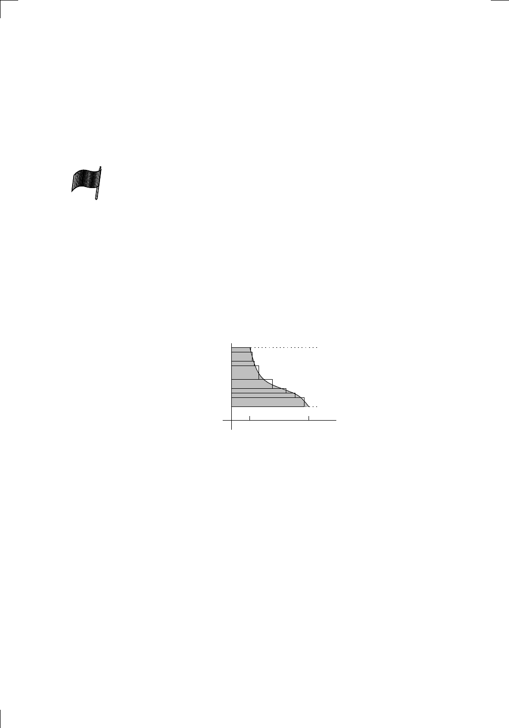
Section 29.1.4: Variation 1: regions between a curve and the y-axis • 623
3. The axis of revolution may be parallel to the x-axis or y-axis, not the
axis itself.
Any combination of these cases can be handled by taking a typical strip and
revolving it appropriately, then integrating; before we see how, it’s important
to know how to decide whether to use the disc method or the shell method.
Notice that when you use the disc method, the strips are revolved about an
axis parallel to their short sides; whereas when you use the shell method, the
strips are revolved about an axis perpendicular to their short sides. That is,
after you carve up the region into little strips, then:
PSfrag replacements
(
a, b)
[
a, b]
(
a, b]
[
a, b)
(
a, ∞)
[
a, ∞)
(
−∞, b)
(
−∞, b]
(
−∞, ∞)
{
x : a < x < b}
{
x : a ≤ x ≤ b}
{
x : a < x ≤ b}
{
x : a ≤ x < b}
{
x : x ≥ a}
{
x : x > a}
{
x : x ≤ b}
{
x : x < b}
R
a
b
shadow
0
1
4
−
2
3
−
3
g(
x) = x
2
f(
x) = x
3
g(
x) = x
2
f(
x) = x
3
mirror (
y = x)
f
−
1
(x) =
3
√
x
y = h
(x)
y = h
−
1
(x)
y = (
x − 1)
2
−
1
x
Same height
−
x
Same length,
opposite signs
y = −
2x
−
2
1
y =
1
2
x − 1
2
−
1
y = 2
x
y = 10
x
y = 2
−
x
y = log
2
(
x)
4
3 units
mirror (
x-axis)
y = |
x|
y = |
log
2
(x)|
θ radians
θ units
30
◦
=
π
6
45
◦
=
π
4
60
◦
=
π
3
120
◦
=
2
π
3
135
◦
=
3
π
4
150
◦
=
5
π
6
90
◦
=
π
2
180
◦
= π
210
◦
=
7
π
6
225
◦
=
5
π
4
240
◦
=
4
π
3
270
◦
=
3
π
2
300
◦
=
5
π
3
315
◦
=
7
π
4
330
◦
=
11
π
6
0
◦
= 0 radians
θ
hyp
otenuse
opposite
adjacent
0 (
≡ 2π)
π
2
π
3
π
2
I
II
III
IV
θ
(
x, y)
x
y
r
7
π
6
reference angle
reference angle =
π
6
sin +
sin −
cos +
cos −
tan +
tan −
A
S
T
C
7
π
4
9
π
13
5
π
6
(this angle is
5
π
6
clockwise)
1
2
1
2
3
4
5
6
0
−
1
−
2
−
3
−
4
−
5
−
6
−
3π
−
5
π
2
−
2π
−
3
π
2
−
π
−
π
2
3
π
3
π
5
π
2
2
π
3
π
2
π
π
2
y = sin(
x)
1
0
−
1
−
3π
−
5
π
2
−
2π
−
3
π
2
−
π
−
π
2
3
π
5
π
2
2
π
2
π
3
π
2
π
π
2
y = sin(
x)
y = cos(
x)
−
π
2
π
2
y = tan(
x), −
π
2
< x <
π
2
0
−
π
2
π
2
y = tan(
x)
−
2π
−
3π
−
5
π
2
−
3
π
2
−
π
−
π
2
π
2
3
π
3
π
5
π
2
2
π
3
π
2
π
y = sec(
x)
y = csc(
x)
y = cot(
x)
y = f (
x)
−
1
1
2
y = g(
x)
3
y = h
(x)
4
5
−
2
f(
x) =
1
x
g(
x) =
1
x
2
etc.
0
1
π
1
2
π
1
3
π
1
4
π
1
5
π
1
6
π
1
7
π
g(
x) = sin
1
x
1
0
−
1
L
10
100
200
y =
π
2
y = −
π
2
y = tan
−
1
(x)
π
2
π
y =
sin(
x)
x
, x > 3
0
1
−
1
a
L
f(
x) = x sin (1/x)
(0 < x < 0
.3)
h
(x) = x
g(
x) = −x
a
L
lim
x
→a
+
f(x) = L
lim
x
→a
+
f(x) = ∞
lim
x
→a
+
f(x) = −∞
lim
x
→a
+
f(x) DNE
lim
x
→a
−
f(x) = L
lim
x
→a
−
f(x) = ∞
lim
x
→a
−
f(x) = −∞
lim
x
→a
−
f(x) DNE
M
}
lim
x
→a
−
f(x) = M
lim
x
→a
f(x) = L
lim
x
→a
f(x) DNE
lim
x
→∞
f(x) = L
lim
x
→∞
f(x) = ∞
lim
x
→∞
f(x) = −∞
lim
x
→∞
f(x) DNE
lim
x
→−∞
f(x) = L
lim
x
→−∞
f(x) = ∞
lim
x
→−∞
f(x) = −∞
lim
x
→−∞
f(x) DNE
lim
x →a
+
f(
x) = ∞
lim
x →a
+
f(
x) = −∞
lim
x →a
−
f(
x) = ∞
lim
x →a
−
f(
x) = −∞
lim
x →a
f(
x) = ∞
lim
x →a
f(
x) = −∞
lim
x →a
f(
x) DNE
y = f (
x)
a
y =
|
x|
x
1
−
1
y =
|
x + 2|
x + 2
1
−
1
−
2
1
2
3
4
a
a
b
y = x sin
1
x
y = x
y = −
x
a
b
c
d
C
a
b
c
d
−
1
0
1
2
3
time
y
t
u
(
t, f(t))
(
u, f(u))
time
y
t
u
y
x
(
x, f(x))
y = |
x|
(
z, f(z))
z
y = f (
x)
a
tangent at x = a
b
tangent at x = b
c
tangent at x = c
y = x
2
tangent
at x = −
1
u
v
uv
u + ∆
u
v + ∆
v
(
u + ∆u)(v + ∆v)
∆
u
∆
v
u
∆v
v∆
u
∆
u∆v
y = f (
x)
1
2
−
2
y = |
x
2
− 4|
y = x
2
− 4
y = −
2x + 5
y = g(
x)
1
2
3
4
5
6
7
8
9
0
−
1
−
2
−
3
−
4
−
5
−
6
y = f (
x)
3
−
3
3
−
3
0
−
1
2
easy
hard
flat
y = f
0
(
x)
3
−
3
0
−
1
2
1
−
1
y = sin(
x)
y = x
x
A
B
O
1
C
D
sin(
x)
tan(
x)
y =
sin(
x)
x
π
2
π
1
−
1
x = 0
a = 0
x > 0
a > 0
x < 0
a < 0
rest position
+
−
y = x
2
sin
1
x
N
A
B
H
a
b
c
O
H
A
B
C
D
h
r
R
θ
1000
2000
α
β
p
h
y = g(
x) = log
b
(x)
y = f (
x) = b
x
y = e
x
5
10
1
2
3
4
0
−
1
−
2
−
3
−
4
y = ln(
x)
y = cosh(
x)
y = sinh(
x)
y = tanh(
x)
y = sech(
x)
y = csch(
x)
y = coth(
x)
1
−
1
y = f (
x)
original function
inverse function
slope = 0 at (
x, y)
slope is infinite at (
y, x)
−
108
2
5
1
2
1
2
3
4
5
6
0
−
1
−
2
−
3
−
4
−
5
−
6
−
3π
−
5
π
2
−
2π
−
3
π
2
−
π
−
π
2
3
π
3
π
5
π
2
2
π
3
π
2
π
π
2
y = sin(
x)
1
0
−
1
−
3π
−
5
π
2
−
2π
−
3
π
2
−
π
−
π
2
3
π
5
π
2
2
π
2
π
3
π
2
π
π
2
y = sin(
x)
y = sin(
x), −
π
2
≤ x ≤
π
2
−
2
−
1
0
2
π
2
−
π
2
y = sin
−
1
(x)
y = cos(
x)
π
π
2
y = cos
−
1
(x)
−
π
2
1
x
α
β
y = tan(
x)
y = tan(
x)
1
y = tan
−
1
(x)
y = sec(
x)
y = sec
−
1
(x)
y = csc
−
1
(x)
y = cot
−
1
(x)
1
y = cosh
−
1
(x)
y = sinh
−
1
(x)
y = tanh
−
1
(x)
y = sech
−
1
(x)
y = csch
−
1
(x)
y = coth
−
1
(x)
(0
, 3)
(2
, −1)
(5
, 2)
(7
, 0)
(
−1, 44)
(0
, 1)
(1
, −12)
(2
, 305)
y = 1
2
(2
, 3)
y = f (
x)
y = g(
x)
a
b
c
a
b
c
s
c
0
c
1
(
a, f(a))
(
b, f(b))
1
2
1
2
3
4
5
6
0
−
1
−
2
−
3
−
4
−
5
−
6
−
3π
−
5
π
2
−
2π
−
3
π
2
−
π
−
π
2
3
π
3
π
5
π
2
2
π
3
π
2
π
π
2
y = sin(
x)
1
0
−
1
−
3π
−
5
π
2
−
2π
−
3
π
2
−
π
−
π
2
3
π
5
π
2
2
π
2
π
3
π
2
π
π
2
c
OR
Local maximum
Local minimum
Horizontal point of inflection
1
e
y = f
0
(
x)
y = f(
x) = x ln(x)
−
1
e
?
y = f(
x) = x
3
y = g(
x) = x
4
x
f(
x)
−
3
−
2
−
1
0
1
2
1
2
3
4
+
−
?
1
5
6
3
f
0
(
x)
2 −
1
2
√
6
2 +
1
2
√
6
f
00
(
x)
7
8
g
00
(
x)
f
00
(
x)
0
y =
(
x − 3)(x − 1)
2
x
3
(
x + 2)
y = x ln(
x)
1
e
−
1
e
5
−
108
2
α
β
2 −
1
2
√
6
2 +
1
2
√
6
y = x
2
(
x − 5)
3
−
e
−
1/2
√
3
e
−
1/2
√
3
−
e
−3/2
e
−
3/2
−
1
√
3
1
√
3
−
1
1
y = xe
−
3x
2
/2
y =
x
3
− 6
x
2
+ 13x − 8
x
28
2
600
500
400
300
200
100
0
−
100
−
200
−
300
−
400
−
500
−
600
0
10
−
10
5
−
5
20
−
20
15
−
15
0
4
5
6
x
P
0
(
x)
+
−
−
existing fence
new fence
enclosure
A
h
b
H
99
100
101
h
dA/dh
r
h
1
2
7
shallow
deep
LAND
SEA
N
y
z
s
t
3
11
9
L
(11)
√
11
y = L
(x)
y = f (
x)
11
y = L
(x)
y = f (
x)
F
P
a
a + ∆
x
f(
a + ∆x)
L
(a + ∆x)
f(
a)
error
df
∆
x
a
b
y = f (
x)
true zero
starting approximation
better approximation
v
t
3
5
50
40
60
4
20
30
25
t
1
t
2
t
3
t
4
t
n
−2
t
n
−1
t
0
= a
t
n
= b
v
1
v
2
v
3
v
4
v
n
−1
v
n
−
30
6
30
|
v|
a
b
p
q
c
v(
c)
v(
c
1
)
v(
c
2
)
v(
c
3
)
v(
c
4
)
v(
c
5
)
v(
c
6
)
t
1
t
2
t
3
t
4
t
5
c
1
c
2
c
3
c
4
c
5
c
6
t
0
=
a
t
6
=
b
t
16
=
b
t
10
=
b
a
b
x
y
y = f (
x)
1
2
y = x
5
0
−
2
y = 1
a
b
y = sin(
x)
π
−
π
0
−
1
−
2
0
2
4
y = x
2
0
1
2
3
4
2
n
4
n
6
n
2(
n−2)
n
2(
n−1)
n
2
n
n
= 2
width of each interval =
2
n
−
2
1
3
0
I
II
III
IV
4
y
dx
y = −
x
2
− 2x + 3
3
−
5
y = |−
x
2
− 2x + 3|
I
II
IIa
5
3
0
1
2
a
b
y = f (
x)
y = g(
x)
y = x
2
a
b
5
3
0
1
2
y =
√
x
2
√
2
2
2
dy
x
2
a
b
y = f (
x)
y = g(
x)
M
m
1
2
−
1
−
2
0
y = e
−
x
2
1
2
e
−
1/4
f
av
y = f
av
c
A
M
0
1
2
a
b
x
t
y = f(
t)
F (
x )
y = f(
t)
F (
x + h )
x + h
F (
x + h) − F (x)
f(
x)
1
2
y = sin(
x)
π
−
π
−
1
−
2
y =
1
x
y = x
2
1
2
1
−
1
y = ln
|x|
θ
a
x
a
x
p
a
2
− x
2
3
x
p
9 − x
2
p
x
2
+ a
2
x
a
p
x
2
+ 15
x
√
15
x
p
x
2
− a
2
a
x
p
x
2
− 4
2
x
−
p
x
2
− a
2
a
x
−
p
x
2
− 4
2
y = f (
x)
a
b
a + ε
ε
Z
b
a
+ε
f(x) dx
small
even smaller
y = g(
x)
infinite area
finite area
1
y =
1
x
y =
1
x
p
, p < 1 (typical)
y =
1
x
p
, p > 1 (typical)
a
1
a
2
a
3
a
4
a
5
a
6
a
7
a
8
1
2
3
4
5
6
7
8
n
a
n
x
y
y = f (
x)
(
a, f(a))
a
−
1
0
1
a
6
1
2
7
1
2
7
?
−
2
−
1
−
2
t = 0
t = π/
6
t = π/
4
t = π/
3
t = π/
2
3
0
t = −
2
t = −
3/2
t = ±
1
t = −
1/2
t = 0
t = 1
/2
t = 3
/2
t = 2
12
−
12
θ
r
P
θ
r
P
11
π
6
2
(
−1, −1)
wrong point
π
4
5
π
4
√
2
(0
, 1)
(0
, −3)
(
−2, 0)
π
2
3
π
2
π
r = 3 sin(
θ)
3
π
2
θ
2
π
1
0
−
1
−
2
−
3
0
3
2
−
3
2
0
r = 1 + 2 cos(
θ)
2
π
3
4
π
3
0
π
0
pi
−
3
2
3
π
2
1
2
3
0
−
1
−
2
−
3
0 ≤ θ ≤
2
π
3
0 ≤ θ ≤ π
0 ≤ θ ≤ 2
π
r = 1 + cos(
θ)
r = 1 +
3
4
cos(
θ)
−
1
4
r = sin(2
θ)
r = sin(3
θ)
r =
1
π
θ
0 ≤ θ ≤ 4
π
r =
2
1 + sin(
θ)
−
π
4
≤ θ ≤
5
π
4
0 ≤ θ ≤ 2
π
0 ≤ θ ≤ π
−
4
−
5
4
5
f(
θ)
f(
θ + dθ)
θ
dθ
θ + dθ
approximating region
exact region
0 ≤ θ ≤ 2π
r = |1 + 2 cos(θ)|
2i
2 − 3i
−1
θ = 0
θ =
π
4
θ =
π
2
θ =
2π
3
θ = π
θ =
13π
12
θ =
3π
2
θ =
7π
4
1 = e
0
e
i
π
4
i = e
i
π
2
e
i
2π
3
−1 = e
iπ
e
i
13π
12
−i = e
i
3π
2
e
i
7π
4
i
−i
1
θ
1 − i
2i
−2i
2
−2
6i
−6i
6
−6
−
√
3
R
ϕ
2
1/5
θ =
π
6
θ =
17π
30
θ =
29π
30
θ =
41π
30
θ =
53π
30
z
0
z
1
z
2
z
3
z
4
−
√
3
2
√
3
2
1
2
i
−i
19π
6
−i
7π
6
i
5π
6
i
17π
6
i
29π
6
ln(2)
−
7π
4
−
3π
4
π
4
5π
4
9π
4
3
2
i
0
1
2
3
4
dx
y
x
y =
p
1 − (x − 3)
2
2πx
a
b
y = f (x)
• if the really thin bit of each strip is parallel to the axis of revolution,
the disc method applies;
• whereas if the really thin bit of each strip is perpendicular to the axis
of revolution, the shell method applies.
Armed with this knowledge, we can now look at our three variations one by
one.
29.1.4 Variation 1: regions between a curve and the y-axis
If the region is between the curve and the y-axis, you probably want to take
strips lying on their sides, with the thin part of the strip along the y-axis:
PSfrag replacements
(
a, b)
[
a, b]
(
a, b]
[
a, b)
(
a, ∞)
[
a, ∞)
(
−∞, b)
(
−∞, b]
(
−∞, ∞)
{
x : a < x < b}
{
x : a ≤ x ≤ b}
{
x : a < x ≤ b}
{
x : a ≤ x < b}
{
x : x ≥ a}
{
x : x > a}
{
x : x ≤ b}
{
x : x < b}
R
a
b
shadow
0
1
4
−
2
3
−
3
g(
x) = x
2
f(
x) = x
3
g(
x) = x
2
f(
x) = x
3
mirror (
y = x)
f
−
1
(x) =
3
√
x
y = h
(x)
y = h
−
1
(x)
y = (
x − 1)
2
−
1
x
Same height
−
x
Same length,
opposite signs
y = −
2x
−
2
1
y =
1
2
x − 1
2
−
1
y = 2
x
y = 10
x
y = 2
−
x
y = log
2
(
x)
4
3 units
mirror (
x-axis)
y = |
x|
y = |
log
2
(x)|
θ radians
θ units
30
◦
=
π
6
45
◦
=
π
4
60
◦
=
π
3
120
◦
=
2
π
3
135
◦
=
3
π
4
150
◦
=
5
π
6
90
◦
=
π
2
180
◦
= π
210
◦
=
7
π
6
225
◦
=
5
π
4
240
◦
=
4
π
3
270
◦
=
3
π
2
300
◦
=
5
π
3
315
◦
=
7
π
4
330
◦
=
11
π
6
0
◦
= 0 radians
θ
hyp
otenuse
opposite
adjacent
0 (
≡ 2π)
π
2
π
3
π
2
I
II
III
IV
θ
(
x, y)
x
y
r
7
π
6
reference angle
reference angle =
π
6
sin +
sin −
cos +
cos −
tan +
tan −
A
S
T
C
7
π
4
9
π
13
5
π
6
(this angle is
5
π
6
clockwise)
1
2
1
2
3
4
5
6
0
−
1
−
2
−
3
−
4
−
5
−
6
−
3π
−
5
π
2
−
2π
−
3
π
2
−
π
−
π
2
3
π
3
π
5
π
2
2
π
3
π
2
π
π
2
y = sin(
x)
1
0
−
1
−
3π
−
5
π
2
−
2π
−
3
π
2
−
π
−
π
2
3
π
5
π
2
2
π
2
π
3
π
2
π
π
2
y = sin(
x)
y = cos(
x)
−
π
2
π
2
y = tan(
x), −
π
2
< x <
π
2
0
−
π
2
π
2
y = tan(
x)
−
2π
−
3π
−
5
π
2
−
3
π
2
−
π
−
π
2
π
2
3
π
3
π
5
π
2
2
π
3
π
2
π
y = sec(
x)
y = csc(
x)
y = cot(
x)
y = f(
x)
−
1
1
2
y = g(
x)
3
y = h
(x)
4
5
−
2
f(
x) =
1
x
g(
x) =
1
x
2
etc.
0
1
π
1
2
π
1
3
π
1
4
π
1
5
π
1
6
π
1
7
π
g(
x) = sin
1
x
1
0
−
1
L
10
100
200
y =
π
2
y = −
π
2
y = tan
−
1
(x)
π
2
π
y =
sin(
x)
x
, x > 3
0
1
−
1
a
L
f(
x) = x sin (1/x)
(0 < x < 0
.3)
h
(x) = x
g(
x) = −x
a
L
lim
x
→a
+
f(x) = L
lim
x
→a
+
f(x) = ∞
lim
x
→a
+
f(x) = −∞
lim
x
→a
+
f(x) DNE
lim
x
→a
−
f(x) = L
lim
x
→a
−
f(x) = ∞
lim
x
→a
−
f(x) = −∞
lim
x
→a
−
f(x) DNE
M
}
lim
x
→a
−
f(x) = M
lim
x
→a
f(x) = L
lim
x
→a
f(x) DNE
lim
x
→∞
f(x) = L
lim
x
→∞
f(x) = ∞
lim
x
→∞
f(x) = −∞
lim
x
→∞
f(x) DNE
lim
x
→−∞
f(x) = L
lim
x
→−∞
f(x) = ∞
lim
x
→−∞
f(x) = −∞
lim
x
→−∞
f(x) DNE
lim
x →a
+
f(
x) = ∞
lim
x →a
+
f(
x) = −∞
lim
x →a
−
f(
x) = ∞
lim
x →a
−
f(
x) = −∞
lim
x →a
f(
x) = ∞
lim
x →a
f(
x) = −∞
lim
x →a
f(
x) DNE
y = f (
x)
a
y =
|
x|
x
1
−
1
y =
|
x + 2|
x + 2
1
−
1
−
2
1
2
3
4
a
a
b
y = x sin
1
x
y = x
y = −
x
a
b
c
d
C
a
b
c
d
−
1
0
1
2
3
time
y
t
u
(
t, f(t))
(
u, f(u))
time
y
t
u
y
x
(
x, f(x))
y = |
x|
(
z, f(z))
z
y = f(
x)
a
tangent at x = a
b
tangent at x = b
c
tangent at x = c
y = x
2
tangent
at x = −
1
u
v
uv
u + ∆
u
v + ∆
v
(
u + ∆u)(v + ∆v)
∆
u
∆
v
u
∆v
v∆
u
∆
u∆v
y = f(
x)
1
2
−
2
y = |
x
2
− 4|
y = x
2
− 4
y = −
2x + 5
y = g(
x)
1
2
3
4
5
6
7
8
9
0
−
1
−
2
−
3
−
4
−
5
−
6
y = f(
x)
3
−
3
3
−
3
0
−
1
2
easy
hard
flat
y = f
0
(
x)
3
−
3
0
−
1
2
1
−
1
y = sin(
x)
y = x
x
A
B
O
1
C
D
sin(
x)
tan(
x)
y =
sin(
x)
x
π
2
π
1
−
1
x = 0
a = 0
x > 0
a > 0
x < 0
a < 0
rest position
+
−
y = x
2
sin
1
x
N
A
B
H
a
b
c
O
H
A
B
C
D
h
r
R
θ
1000
2000
α
β
p
h
y = g(
x) = log
b
(x)
y = f (
x) = b
x
y = e
x
5
10
1
2
3
4
0
−
1
−
2
−
3
−
4
y = ln(
x)
y = cosh(
x)
y = sinh(
x)
y = tanh(
x)
y = sech(
x)
y = csch(
x)
y = coth(
x)
1
−
1
y = f(
x)
original function
inverse function
slope = 0 at (
x, y)
slope is infinite at (
y, x)
−
108
2
5
1
2
1
2
3
4
5
6
0
−
1
−
2
−
3
−
4
−
5
−
6
−
3π
−
5
π
2
−
2π
−
3
π
2
−
π
−
π
2
3
π
3
π
5
π
2
2
π
3
π
2
π
π
2
y = sin(
x)
1
0
−
1
−
3π
−
5
π
2
−
2π
−
3
π
2
−
π
−
π
2
3
π
5
π
2
2
π
2
π
3
π
2
π
π
2
y = sin(
x)
y = sin(
x), −
π
2
≤ x ≤
π
2
−
2
−
1
0
2
π
2
−
π
2
y = sin
−
1
(x)
y = cos(
x)
π
π
2
y = cos
−
1
(x)
−
π
2
1
x
α
β
y = tan(
x)
y = tan(
x)
1
y = tan
−
1
(x)
y = sec(
x)
y = sec
−
1
(x)
y = csc
−
1
(x)
y = cot
−
1
(x)
1
y = cosh
−
1
(x)
y = sinh
−
1
(x)
y = tanh
−
1
(x)
y = sech
−
1
(x)
y = csch
−
1
(x)
y = coth
−
1
(x)
(0
, 3)
(2
, −1)
(5
, 2)
(7
, 0)
(
−1, 44)
(0
, 1)
(1
, −12)
(2
, 305)
y = 1
2
(2
, 3)
y = f(
x)
y = g(
x)
a
b
c
a
b
c
s
c
0
c
1
(
a, f(a))
(
b, f(b))
1
2
1
2
3
4
5
6
0
−
1
−
2
−
3
−
4
−
5
−
6
−
3π
−
5
π
2
−
2π
−
3
π
2
−
π
−
π
2
3
π
3
π
5
π
2
2
π
3
π
2
π
π
2
y = sin(
x)
1
0
−
1
−
3π
−
5
π
2
−
2π
−
3
π
2
−
π
−
π
2
3
π
5
π
2
2
π
2
π
3
π
2
π
π
2
c
OR
Local maximum
Local minimum
Horizontal point of inflection
1
e
y = f
0
(
x)
y = f(
x) = x ln(x)
−
1
e
?
y = f (
x) = x
3
y = g(
x) = x
4
x
f(
x)
−
3
−
2
−
1
0
1
2
1
2
3
4
+
−
?
1
5
6
3
f
0
(
x)
2 −
1
2
√
6
2 +
1
2
√
6
f
00
(
x)
7
8
g
00
(
x)
f
00
(
x)
0
y =
(
x − 3)(x − 1)
2
x
3
(
x + 2)
y = x ln(
x)
1
e
−
1
e
5
−
108
2
α
β
2 −
1
2
√
6
2 +
1
2
√
6
y = x
2
(
x − 5)
3
−
e
−
1/2
√
3
e
−
1/2
√
3
−
e
−3/2
e
−
3/2
−
1
√
3
1
√
3
−
1
1
y = xe
−
3x
2
/2
y =
x
3
− 6
x
2
+ 13x − 8
x
28
2
600
500
400
300
200
100
0
−
100
−
200
−
300
−
400
−
500
−
600
0
10
−
10
5
−
5
20
−
20
15
−
15
0
4
5
6
x
P
0
(
x)
+
−
−
existing fence
new fence
enclosure
A
h
b
H
99
100
101
h
dA/dh
r
h
1
2
7
shallow
deep
LAND
SEA
N
y
z
s
t
3
11
9
L
(11)
√
11
y = L
(x)
y = f(
x)
11
y = L
(x)
y = f(
x)
F
P
a
a + ∆
x
f(
a + ∆x)
L
(a + ∆x)
f(
a)
error
df
∆
x
a
b
y = f(
x)
true zero
starting approximation
better approximation
v
t
3
5
50
40
60
4
20
30
25
t
1
t
2
t
3
t
4
t
n
−2
t
n
−1
t
0
= a
t
n
= b
v
1
v
2
v
3
v
4
v
n
−1
v
n
−
30
6
30
|
v|
a
b
p
q
c
v(
c)
v(
c
1
)
v(
c
2
)
v(
c
3
)
v(
c
4
)
v(
c
5
)
v(
c
6
)
t
1
t
2
t
3
t
4
t
5
c
1
c
2
c
3
c
4
c
5
c
6
t
0
=
a
t
6
=
b
t
16
=
b
t
10
=
b
a
b
x
y
y = f(
x)
1
2
y = x
5
0
−
2
y = 1
a
b
y = sin(
x)
π
−
π
0
−
1
−
2
0
2
4
y = x
2
0
1
2
3
4
2
n
4
n
6
n
2(
n−2)
n
2(
n−1)
n
2
n
n
= 2
width of each interval =
2
n
−
2
1
3
0
I
II
III
IV
4
y
dx
y = −
x
2
− 2x + 3
3
−
5
y = |−
x
2
− 2x + 3|
I
II
IIa
5
3
0
1
2
a
b
y = f(
x)
y = g(
x)
y = x
2
a
b
5
3
0
1
2
y =
√
x
2
√
2
2
2
dy
x
2
a
b
y = f(
x)
y = g(
x)
M
m
1
2
−
1
−
2
0
y = e
−
x
2
1
2
e
−
1/4
f
av
y = f
av
c
A
M
0
1
2
a
b
x
t
y = f(
t)
F (
x )
y = f(
t)
F (
x + h )
x + h
F (
x + h) − F (x)
f(
x)
1
2
y = sin(
x)
π
−
π
−
1
−
2
y =
1
x
y = x
2
1
2
1
−
1
y = ln|
x|
θ
a
x
a
x
p
a
2
− x
2
3
x
p
9 − x
2
p
x
2
+ a
2
x
a
p
x
2
+ 15
x
√
15
x
p
x
2
− a
2
a
x
p
x
2
− 4
2
x
−
p
x
2
− a
2
a
x
−
p
x
2
− 4
2
y = f(
x)
a
b
a + ε
ε
Z
b
a
+ε
f(x) dx
small
even smaller
y = g(
x)
infinite area
finite area
1
y =
1
x
y =
1
x
p
, p < 1 (typical)
y =
1
x
p
, p > 1 (typical)
a
1
a
2
a
3
a
4
a
5
a
6
a
7
a
8
1
2
3
4
5
6
7
8
n
a
n
x
y
y = f(
x)
(
a, f(a))
a
−
1
0
1
a
6
1
2
7
1
2
7
?
−
2
−
1
−
2
t = 0
t = π/
6
t = π/
4
t = π/
3
t = π/
2
3
0
t = −
2
t = −
3/2
t = ±
1
t = −
1/2
t = 0
t = 1
/2
t = 3
/2
t = 2
12
−
12
θ
r
P
θ
r
P
11
π
6
2
(
−1, −1)
wrong point
π
4
5
π
4
√
2
(0
, 1)
(0
, −3)
(
−2, 0)
π
2
3
π
2
π
r = 3 sin(
θ)
3
π
2
θ
2
π
1
0
−
1
−
2
−
3
0
3
2
−
3
2
0
r = 1 + 2 cos(
θ)
2
π
3
4
π
3
0
π
0
pi
−
3
2
3
π
2
1
2
3
0
−
1
−
2
−
3
0 ≤ θ ≤
2
π
3
0 ≤ θ ≤ π
0 ≤ θ ≤ 2
π
r = 1 + cos(
θ)
r = 1 +
3
4
cos(
θ)
−
1
4
r = sin(2
θ)
r = sin(3
θ)
r =
1
π
θ
0 ≤ θ ≤ 4π
r =
2
1 + sin(θ)
−
π
4
≤ θ ≤
5π
4
0 ≤ θ ≤ 2π
0 ≤ θ ≤ π
−4
−5
4
5
f(θ)
f(θ + dθ)
θ
dθ
θ + dθ
approximating region
exact region
0 ≤ θ ≤ 2π
r = |1 + 2 cos(θ)|
2i
2 − 3i
−1
θ = 0
θ =
π
4
θ =
π
2
θ =
2π
3
θ = π
θ =
13π
12
θ =
3π
2
θ =
7π
4
1 = e
0
e
i
π
4
i = e
i
π
2
e
i
2π
3
−1 = e
iπ
e
i
13π
12
−i = e
i
3π
2
e
i
7π
4
i
−i
1
θ
1 − i
2i
−2i
2
−2
6i
−6i
6
−6
−
√
3
R
ϕ
2
1/5
θ =
π
6
θ =
17π
30
θ =
29π
30
θ =
41π
30
θ =
53π
30
z
0
z
1
z
2
z
3
z
4
−
√
3
2
√
3
2
1
2
i
−i
19π
6
−i
7π
6
i
5π
6
i
17π
6
i
29π
6
ln(2)
−
7π
4
−
3π
4
π
4
5π
4
9π
4
3
2
i
0
1
2
3
4
dx
y
x
y =
p
1 − (x − 3)
2
2πx
a
b
y = f(x)
A
B
We actually did the same thing when we saw how to find the area of a re-
gion bounded by some curve and the y-axis, way back in Section 16.4.3 of
Chapter 16. In any case, suppose that you want to find the volume of the
solid formed by revolving this region about the y-axis. You should use the
disc method, since the thin side of the strip is parallel to that axis. A typical
strip at position y has width dy and length x units, so the resulting disc has
volume πx
2
dy cubic units. When you integrate this to find the total volume,
be very careful that the limits of integration are relevant points on the y-axis,
not the x-axis, since the integral is taken with respect to y (because of the
dy). In particular, we need the integral to go from A to B, not a to b (see the
above diagram), so the volume we want is
R
B
A
πx
2
dy.
There’s another way to look at this. Look at the above picture and rest
your head on your right shoulder. The y-axis becomes horizontal, but ev-
erything’s back to front, so try to visualize what would happen if the page
were transparent and you looked at the diagram in reverse (still with your
head tipped over). Now the y-axis and x-axis have switched places! This sug-
gests that you can just switch the variables x and y wherever you see them,
provided that you also make the bounds of integration refer to points on the
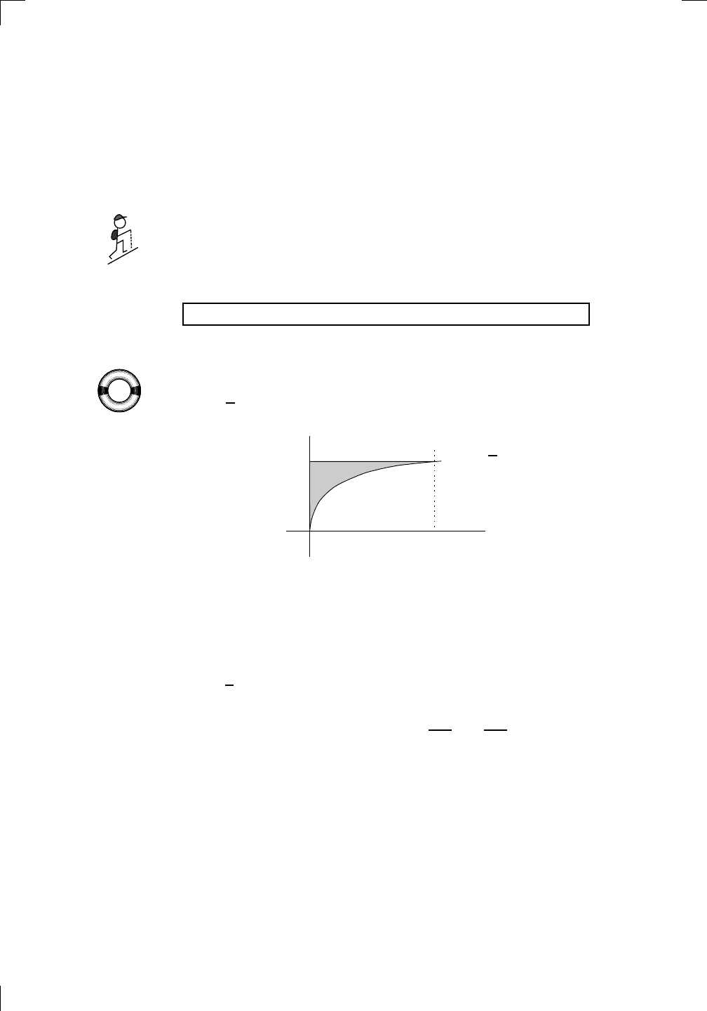
624 • Volumes, Arc Lengths, and Surface Areas
y-axis. Indeed, if we do this to our formula V =
R
b
a
πy
2
dx from Section 29.1.3
above, we see that the volume of a region down to the y-axis revolved about
the y-axis is
R
B
A
πx
2
dy, which agrees with what we’ve seen above.
How about if the above region is revolved about the x-axis, instead of the
y-axis? Simply adapt the shell formula V =
R
b
a
2πxy dx from Section 29.1.3
above to see that the volume we want is
R
B
A
2πyx dy. This makes sense, since
revolving a typical strip about the x-axis gives a shell with thickness dy, height
x, and radius y units. You should draw what happens when you unfold such a
PSfrag
replacements
(
a, b)
[
a, b]
(
a, b]
[
a, b)
(
a, ∞)
[
a, ∞)
(
−∞, b)
(
−∞, b]
(
−∞, ∞)
{
x : a < x < b}
{
x : a ≤ x ≤ b}
{
x : a < x ≤ b}
{
x : a ≤ x < b}
{
x : x ≥ a}
{
x : x > a}
{
x : x ≤ b}
{
x : x < b}
R
a
b
shado
w
0
1
4
−
2
3
−
3
g(
x) = x
2
f(
x) = x
3
g(
x) = x
2
f(
x) = x
3
mirror
(y = x)
f
−
1
(x) =
3
√
x
y = h
(x)
y = h
−
1
(x)
y =
(x − 1)
2
−
1
x
Same
height
−
x
Same
length,
opp
osite signs
y = −
2x
−
2
1
y =
1
2
x − 1
2
−
1
y =
2
x
y =
10
x
y =
2
−x
y =
log
2
(x)
4
3
units
mirror
(x-axis)
y = |
x|
y = |
log
2
(x)|
θ radians
θ units
30
◦
=
π
6
45
◦
=
π
4
60
◦
=
π
3
120
◦
=
2
π
3
135
◦
=
3
π
4
150
◦
=
5
π
6
90
◦
=
π
2
180
◦
= π
210
◦
=
7
π
6
225
◦
=
5
π
4
240
◦
=
4
π
3
270
◦
=
3
π
2
300
◦
=
5
π
3
315
◦
=
7
π
4
330
◦
=
11
π
6
0
◦
=
0 radians
θ
hyp
otenuse
opp
osite
adjacen
t
0
(≡ 2π)
π
2
π
3
π
2
I
I
I
I
II
IV
θ
(
x, y)
x
y
r
7
π
6
reference
angle
reference
angle =
π
6
sin
+
sin −
cos
+
cos −
tan
+
tan −
A
S
T
C
7
π
4
9
π
13
5
π
6
(this
angle is
5π
6
clo
ckwise)
1
2
1
2
3
4
5
6
0
−
1
−
2
−
3
−
4
−
5
−
6
−
3π
−
5
π
2
−
2π
−
3
π
2
−
π
−
π
2
3
π
3
π
5
π
2
2
π
3
π
2
π
π
2
y =
sin(x)
1
0
−
1
−
3π
−
5
π
2
−
2π
−
3
π
2
−
π
−
π
2
3
π
5
π
2
2
π
2
π
3
π
2
π
π
2
y =
sin(x)
y =
cos(x)
−
π
2
π
2
y =
tan(x), −
π
2
<
x <
π
2
0
−
π
2
π
2
y =
tan(x)
−
2π
−
3π
−
5
π
2
−
3
π
2
−
π
−
π
2
π
2
3
π
3
π
5
π
2
2
π
3
π
2
π
y =
sec(x)
y =
csc(x)
y =
cot(x)
y = f(
x)
−
1
1
2
y = g(
x)
3
y = h
(x)
4
5
−
2
f(
x) =
1
x
g(
x) =
1
x
2
etc.
0
1
π
1
2
π
1
3
π
1
4
π
1
5
π
1
6
π
1
7
π
g(
x) = sin
1
x
1
0
−
1
L
10
100
200
y =
π
2
y = −
π
2
y =
tan
−1
(x)
π
2
π
y =
sin(
x)
x
,
x > 3
0
1
−
1
a
L
f(
x) = x sin (1/x)
(0 <
x < 0.3)
h
(x) = x
g(
x) = −x
a
L
lim
x
→a
+
f(x) = L
lim
x
→a
+
f(x) = ∞
lim
x
→a
+
f(x) = −∞
lim
x
→a
+
f(x) DNE
lim
x
→a
−
f(x) = L
lim
x
→a
−
f(x) = ∞
lim
x
→a
−
f(x) = −∞
lim
x
→a
−
f(x) DNE
M
}
lim
x
→a
−
f(x) = M
lim
x
→a
f(x) = L
lim
x
→a
f(x) DNE
lim
x
→∞
f(x) = L
lim
x
→∞
f(x) = ∞
lim
x
→∞
f(x) = −∞
lim
x
→∞
f(x) DNE
lim
x
→−∞
f(x) = L
lim
x
→−∞
f(x) = ∞
lim
x
→−∞
f(x) = −∞
lim
x
→−∞
f(x) DNE
lim
x →a
+
f(
x) = ∞
lim
x →a
+
f(
x) = −∞
lim
x →a
−
f(
x) = ∞
lim
x →a
−
f(
x) = −∞
lim
x →a
f(
x) = ∞
lim
x →a
f(
x) = −∞
lim
x →a
f(
x) DNE
y = f (
x)
a
y =
|
x|
x
1
−
1
y =
|
x + 2|
x +
2
1
−
1
−
2
1
2
3
4
a
a
b
y = x sin
1
x
y = x
y = −
x
a
b
c
d
C
a
b
c
d
−
1
0
1
2
3
time
y
t
u
(
t, f(t))
(
u, f(u))
time
y
t
u
y
x
(
x, f(x))
y = |
x|
(
z, f(z))
z
y = f(
x)
a
tangen
t at x = a
b
tangen
t at x = b
c
tangen
t at x = c
y = x
2
tangen
t
at x = −
1
u
v
uv
u +
∆u
v +
∆v
(
u + ∆u)(v + ∆v)
∆
u
∆
v
u
∆v
v∆
u
∆
u∆v
y = f(
x)
1
2
−
2
y = |
x
2
− 4|
y = x
2
− 4
y = −
2x + 5
y = g(
x)
1
2
3
4
5
6
7
8
9
0
−
1
−
2
−
3
−
4
−
5
−
6
y = f (
x)
3
−
3
3
−
3
0
−
1
2
easy
hard
flat
y = f
0
(
x)
3
−
3
0
−
1
2
1
−
1
y =
sin(x)
y = x
x
A
B
O
1
C
D
sin(
x)
tan(
x)
y =
sin(
x)
x
π
2
π
1
−
1
x =
0
a =
0
x
> 0
a
> 0
x
< 0
a
< 0
rest
position
+
−
y = x
2
sin
1
x
N
A
B
H
a
b
c
O
H
A
B
C
D
h
r
R
θ
1000
2000
α
β
p
h
y = g(
x) = log
b
(x)
y = f(
x) = b
x
y = e
x
5
10
1
2
3
4
0
−
1
−
2
−
3
−
4
y =
ln(x)
y =
cosh(x)
y =
sinh(x)
y =
tanh(x)
y =
sech(x)
y =
csch(x)
y =
coth(x)
1
−
1
y = f(
x)
original
function
in
verse function
slop
e = 0 at (x, y)
slop
e is infinite at (y, x)
−
108
2
5
1
2
1
2
3
4
5
6
0
−
1
−
2
−
3
−
4
−
5
−
6
−
3π
−
5
π
2
−
2π
−
3
π
2
−
π
−
π
2
3
π
3
π
5
π
2
2
π
3
π
2
π
π
2
y =
sin(x)
1
0
−
1
−
3π
−
5
π
2
−
2π
−
3
π
2
−
π
−
π
2
3
π
5
π
2
2
π
2
π
3
π
2
π
π
2
y =
sin(x)
y =
sin(x), −
π
2
≤ x ≤
π
2
−
2
−
1
0
2
π
2
−
π
2
y =
sin
−1
(x)
y =
cos(x)
π
π
2
y =
cos
−1
(x)
−
π
2
1
x
α
β
y =
tan(x)
y =
tan(x)
1
y =
tan
−1
(x)
y =
sec(x)
y =
sec
−1
(x)
y =
csc
−1
(x)
y =
cot
−1
(x)
1
y =
cosh
−1
(x)
y =
sinh
−1
(x)
y =
tanh
−1
(x)
y =
sech
−1
(x)
y =
csch
−1
(x)
y =
coth
−1
(x)
(0
, 3)
(2
, −1)
(5
, 2)
(7
, 0)
(
−1, 44)
(0
, 1)
(1
, −12)
(2
, 305)
y =
1
2
(2
, 3)
y = f(
x)
y = g(
x)
a
b
c
a
b
c
s
c
0
c
1
(
a, f(a))
(
b, f(b))
1
2
1
2
3
4
5
6
0
−
1
−
2
−
3
−
4
−
5
−
6
−
3π
−
5
π
2
−
2π
−
3
π
2
−
π
−
π
2
3
π
3
π
5
π
2
2
π
3
π
2
π
π
2
y =
sin(x)
1
0
−
1
−
3π
−
5
π
2
−
2π
−
3
π
2
−
π
−
π
2
3
π
5
π
2
2
π
2
π
3
π
2
π
π
2
c
OR
Lo
cal maximum
Lo
cal minimum
Horizon
tal point of inflection
1
e
y = f
0
(
x)
y = f (
x) = x ln(x)
−
1
e
?
y = f(
x) = x
3
y = g(
x) = x
4
x
f(
x)
−
3
−
2
−
1
0
1
2
1
2
3
4
+
−
?
1
5
6
3
f
0
(
x)
2 −
1
2
√
6
2
+
1
2
√
6
f
00
(
x)
7
8
g
00
(
x)
f
00
(
x)
0
y =
(
x − 3)(x − 1)
2
x
3
(
x + 2)
y = x ln
(x)
1
e
−
1
e
5
−
108
2
α
β
2 −
1
2
√
6
2
+
1
2
√
6
y = x
2
(
x − 5)
3
−
e
−
1/2
√
3
e
−
1/2
√
3
−
e
−3/2
e
−
3/2
−
1
√
3
1
√
3
−
1
1
y = xe
−
3x
2
/2
y =
x
3
− 6
x
2
+ 13x − 8
x
28
2
600
500
400
300
200
100
0
−
100
−
200
−
300
−
400
−
500
−
600
0
10
−
10
5
−
5
20
−
20
15
−
15
0
4
5
6
x
P
0
(
x)
+
−
−
existing
fence
new
fence
enclosure
A
h
b
H
99
100
101
h
dA/dh
r
h
1
2
7
shallo
w
deep
LAND
SEA
N
y
z
s
t
3
11
9
L
(11)
√
11
y = L
(x)
y = f (
x)
11
y = L
(x)
y = f(
x)
F
P
a
a +
∆x
f(
a + ∆x)
L
(a + ∆x)
f(
a)
error
d
f
∆
x
a
b
y = f(
x)
true
zero
starting
approximation
b
etter approximation
v
t
3
5
50
40
60
4
20
30
25
t
1
t
2
t
3
t
4
t
n
−2
t
n
−1
t
0
= a
t
n
= b
v
1
v
2
v
3
v
4
v
n
−1
v
n
−
30
6
30
|
v|
a
b
p
q
c
v(
c)
v(
c
1
)
v(
c
2
)
v(
c
3
)
v(
c
4
)
v(
c
5
)
v(
c
6
)
t
1
t
2
t
3
t
4
t
5
c
1
c
2
c
3
c
4
c
5
c
6
t
0
=
a
t
6
=
b
t
16
=
b
t
10
=
b
a
b
x
y
y = f(
x)
1
2
y = x
5
0
−
2
y =
1
a
b
y =
sin(x)
π
−
π
0
−
1
−
2
0
2
4
y = x
2
0
1
2
3
4
2
n
4
n
6
n
2(
n−2)
n
2(
n−1)
n
2
n
n
=
2
width
of each interval =
2
n
−
2
1
3
0
I
I
I
I
II
IV
4
y
dx
y = −
x
2
− 2x + 3
3
−
5
y = |−
x
2
− 2x + 3|
I
I
I
I
Ia
5
3
0
1
2
a
b
y = f (
x)
y = g(
x)
y = x
2
a
b
5
3
0
1
2
y =
√
x
2
√
2
2
2
dy
x
2
a
b
y = f(
x)
y = g(
x)
M
m
1
2
−
1
−
2
0
y = e
−
x
2
1
2
e
−
1/4
f
a
v
y = f
a
v
c
A
M
0
1
2
a
b
x
t
y = f (
t)
F (
x )
y = f (
t)
F (
x + h)
x + h
F (
x + h) − F (x)
f(
x)
1
2
y =
sin(x)
π
−
π
−
1
−
2
y =
1
x
y = x
2
1
2
1
−
1
y =
ln|x|
θ
a
x
a
x
p
a
2
− x
2
3
x
p
9 − x
2
p
x
2
+ a
2
x
a
p
x
2
+ 15
x
√
15
x
p
x
2
− a
2
a
x
p
x
2
− 4
2
x
−
p
x
2
− a
2
a
x
−
p
x
2
− 4
2
y = f(
x)
a
b
a + ε
ε
Z
b
a
+ε
f(x) dx
small
ev
en smaller
y = g(
x)
infinite
area
finite
area
1
y =
1
x
y =
1
x
p
, p
< 1 (typical)
y =
1
x
p
, p
> 1 (typical)
a
1
a
2
a
3
a
4
a
5
a
6
a
7
a
8
1
2
3
4
5
6
7
8
n
a
n
x
y
y = f(
x)
(
a, f(a))
a
−
1
0
1
a
6
1
2
7
1
2
7
?
−
2
−
1
−
2
t =
0
t = π
/6
t = π
/4
t = π
/3
t = π
/2
3
0
t = −
2
t = −
3/2
t = ±
1
t = −
1/2
t =
0
t =
1/2
t =
3/2
t =
2
12
−
12
θ
r
P
θ
r
P
11
π
6
2
(
−1, −1)
wrong
point
π
4
5
π
4
√
2
(0
, 1)
(0
, −3)
(
−2, 0)
π
2
3
π
2
π
r =
3 sin(θ)
3
π
2
θ
2
π
1
0
−
1
−
2
−
3
0
3
2
−
3
2
0
r =
1 + 2 cos(θ)
2
π
3
4
π
3
0
π
0
pi
−
3
2
3
π
2
1
2
3
0
−
1
−
2
−
3
0 ≤ θ ≤
2
π
3
0 ≤ θ ≤ π
0 ≤ θ ≤ 2
π
r =
1 + cos(θ)
r =
1 +
3
4
cos(
θ)
−
1
4
r =
sin(2θ)
r =
sin(3θ)
r =
1
π
θ
0 ≤ θ ≤ 4
π
r =
2
1
+ sin(θ)
−
π
4
≤ θ ≤
5
π
4
0 ≤ θ ≤ 2
π
0 ≤ θ ≤ π
−
4
−
5
4
5
f(
θ)
f(
θ + dθ)
θ
dθ
θ + dθ
appro
ximating region
exact
region
0 ≤ θ ≤ 2π
r = |1 + 2 cos(θ)|
2i
2 − 3i
−1
θ = 0
θ =
π
4
θ =
π
2
θ =
2π
3
θ = π
θ =
13π
12
θ =
3π
2
θ =
7π
4
1 = e
0
e
i
π
4
i = e
i
π
2
e
i
2π
3
−1 = e
iπ
e
i
13π
12
−i = e
i
3π
2
e
i
7π
4
i
−i
1
θ
1 − i
2i
−2i
2
−2
6i
−6i
6
−6
−
√
3
R
ϕ
2
1/5
θ =
π
6
θ =
17π
30
θ =
29π
30
θ =
41π
30
θ =
53π
30
z
0
z
1
z
2
z
3
z
4
−
√
3
2
√
3
2
1
2
i
−i
19π
6
−i
7π
6
i
5π
6
i
17π
6
i
29π
6
ln(2)
−
7π
4
−
3π
4
π
4
5π
4
9π
4
3
2
i
0
1
2
3
4
dx
y
x
y =
p
1 − (x − 3)
2
2πx
a
b
y = f(x)
A
B
strip into a thin shape which is approximately a rectangular prism, calculate
its volume, and see that you do indeed get 2πyx dy. In summary, then, the
rule of thumb is this:
If the region lies between a curve and the y-axis, switch x and y.
As always, drawing a typical strip, revolving it, calculating the resulting vol-
ume, and integrating is the most reliable way; the above rule of thumb is just
a guide.
Here’s an example of Variation 1. Let R denote the region between the
PSfrag
replacements
(
a, b)
[
a, b]
(
a, b]
[
a, b)
(
a, ∞)
[
a, ∞)
(
−∞, b)
(
−∞, b]
(
−∞, ∞)
{
x : a < x < b}
{
x : a ≤ x ≤ b}
{
x : a < x ≤ b}
{
x : a ≤ x < b}
{
x : x ≥ a}
{
x : x > a}
{
x : x ≤ b}
{
x : x < b}
R
a
b
shado
w
0
1
4
−
2
3
−
3
g(
x) = x
2
f(
x) = x
3
g(
x) = x
2
f(
x) = x
3
mirror
(y = x)
f
−
1
(x) =
3
√
x
y = h
(x)
y = h
−
1
(x)
y =
(x − 1)
2
−
1
x
Same
height
−
x
Same
length,
opp
osite signs
y = −
2x
−
2
1
y =
1
2
x − 1
2
−
1
y =
2
x
y =
10
x
y =
2
−x
y =
log
2
(x)
4
3
units
mirror
(x-axis)
y = |
x|
y = |
log
2
(x)|
θ radians
θ units
30
◦
=
π
6
45
◦
=
π
4
60
◦
=
π
3
120
◦
=
2
π
3
135
◦
=
3
π
4
150
◦
=
5
π
6
90
◦
=
π
2
180
◦
= π
210
◦
=
7
π
6
225
◦
=
5
π
4
240
◦
=
4
π
3
270
◦
=
3
π
2
300
◦
=
5
π
3
315
◦
=
7
π
4
330
◦
=
11
π
6
0
◦
=
0 radians
θ
hyp
otenuse
opp
osite
adjacen
t
0
(≡ 2π)
π
2
π
3
π
2
I
I
I
I
II
IV
θ
(
x, y)
x
y
r
7
π
6
reference
angle
reference
angle =
π
6
sin
+
sin −
cos
+
cos −
tan
+
tan −
A
S
T
C
7
π
4
9
π
13
5
π
6
(this
angle is
5π
6
clo
ckwise)
1
2
1
2
3
4
5
6
0
−
1
−
2
−
3
−
4
−
5
−
6
−
3π
−
5
π
2
−
2π
−
3
π
2
−
π
−
π
2
3
π
3
π
5
π
2
2
π
3
π
2
π
π
2
y =
sin(x)
1
0
−
1
−
3π
−
5
π
2
−
2π
−
3
π
2
−
π
−
π
2
3
π
5
π
2
2
π
2
π
3
π
2
π
π
2
y =
sin(x)
y =
cos(x)
−
π
2
π
2
y =
tan(x), −
π
2
<
x <
π
2
0
−
π
2
π
2
y =
tan(x)
−
2π
−
3π
−
5
π
2
−
3
π
2
−
π
−
π
2
π
2
3
π
3
π
5
π
2
2
π
3
π
2
π
y =
sec(x)
y =
csc(x)
y =
cot(x)
y = f(
x)
−
1
1
2
y = g(
x)
3
y = h
(x)
4
5
−
2
f(
x) =
1
x
g(
x) =
1
x
2
etc.
0
1
π
1
2
π
1
3
π
1
4
π
1
5
π
1
6
π
1
7
π
g(
x) = sin
1
x
1
0
−
1
L
10
100
200
y =
π
2
y = −
π
2
y =
tan
−1
(x)
π
2
π
y =
sin(
x)
x
,
x > 3
0
1
−
1
a
L
f(
x) = x sin (1/x)
(0 <
x < 0.3)
h
(x) = x
g(
x) = −x
a
L
lim
x
→a
+
f(x) = L
lim
x
→a
+
f(x) = ∞
lim
x
→a
+
f(x) = −∞
lim
x
→a
+
f(x) DNE
lim
x
→a
−
f(x) = L
lim
x
→a
−
f(x) = ∞
lim
x
→a
−
f(x) = −∞
lim
x
→a
−
f(x) DNE
M
}
lim
x
→a
−
f(x) = M
lim
x
→a
f(x) = L
lim
x
→a
f(x) DNE
lim
x
→∞
f(x) = L
lim
x
→∞
f(x) = ∞
lim
x
→∞
f(x) = −∞
lim
x
→∞
f(x) DNE
lim
x
→−∞
f(x) = L
lim
x
→−∞
f(x) = ∞
lim
x
→−∞
f(x) = −∞
lim
x
→−∞
f(x) DNE
lim
x →a
+
f(
x) = ∞
lim
x →a
+
f(
x) = −∞
lim
x →a
−
f(
x) = ∞
lim
x →a
−
f(
x) = −∞
lim
x →a
f(
x) = ∞
lim
x →a
f(
x) = −∞
lim
x →a
f(
x) DNE
y = f (
x)
a
y =
|
x|
x
1
−
1
y =
|
x + 2|
x +
2
1
−
1
−
2
1
2
3
4
a
a
b
y = x sin
1
x
y = x
y = −
x
a
b
c
d
C
a
b
c
d
−
1
0
1
2
3
time
y
t
u
(
t, f(t))
(
u, f(u))
time
y
t
u
y
x
(
x, f(x))
y = |
x|
(
z, f(z))
z
y = f(
x)
a
tangen
t at x = a
b
tangen
t at x = b
c
tangen
t at x = c
y = x
2
tangen
t
at x = −
1
u
v
uv
u +
∆u
v +
∆v
(
u + ∆u)(v + ∆v)
∆
u
∆
v
u
∆v
v∆
u
∆
u∆v
y = f(
x)
1
2
−
2
y = |
x
2
− 4|
y = x
2
− 4
y = −
2x + 5
y = g(
x)
1
2
3
4
5
6
7
8
9
0
−
1
−
2
−
3
−
4
−
5
−
6
y = f (
x)
3
−
3
3
−
3
0
−
1
2
easy
hard
flat
y = f
0
(
x)
3
−
3
0
−
1
2
1
−
1
y =
sin(x)
y = x
x
A
B
O
1
C
D
sin(
x)
tan(
x)
y =
sin(
x)
x
π
2
π
1
−
1
x =
0
a =
0
x
> 0
a
> 0
x
< 0
a
< 0
rest
position
+
−
y = x
2
sin
1
x
N
A
B
H
a
b
c
O
H
A
B
C
D
h
r
R
θ
1000
2000
α
β
p
h
y = g(
x) = log
b
(x)
y = f(
x) = b
x
y = e
x
5
10
1
2
3
4
0
−
1
−
2
−
3
−
4
y =
ln(x)
y =
cosh(x)
y =
sinh(x)
y =
tanh(x)
y =
sech(x)
y =
csch(x)
y =
coth(x)
1
−
1
y = f(
x)
original
function
in
verse function
slop
e = 0 at (x, y)
slop
e is infinite at (y, x)
−
108
2
5
1
2
1
2
3
4
5
6
0
−
1
−
2
−
3
−
4
−
5
−
6
−
3π
−
5
π
2
−
2π
−
3
π
2
−
π
−
π
2
3
π
3
π
5
π
2
2
π
3
π
2
π
π
2
y =
sin(x)
1
0
−
1
−
3π
−
5
π
2
−
2π
−
3
π
2
−
π
−
π
2
3
π
5
π
2
2
π
2
π
3
π
2
π
π
2
y =
sin(x)
y =
sin(x), −
π
2
≤ x ≤
π
2
−
2
−
1
0
2
π
2
−
π
2
y =
sin
−1
(x)
y =
cos(x)
π
π
2
y =
cos
−1
(x)
−
π
2
1
x
α
β
y =
tan(x)
y =
tan(x)
1
y =
tan
−1
(x)
y =
sec(x)
y =
sec
−1
(x)
y =
csc
−1
(x)
y =
cot
−1
(x)
1
y =
cosh
−1
(x)
y =
sinh
−1
(x)
y =
tanh
−1
(x)
y =
sech
−1
(x)
y =
csch
−1
(x)
y =
coth
−1
(x)
(0
, 3)
(2
, −1)
(5
, 2)
(7
, 0)
(
−1, 44)
(0
, 1)
(1
, −12)
(2
, 305)
y =
1
2
(2
, 3)
y = f(
x)
y = g(
x)
a
b
c
a
b
c
s
c
0
c
1
(
a, f(a))
(
b, f(b))
1
2
1
2
3
4
5
6
0
−
1
−
2
−
3
−
4
−
5
−
6
−
3π
−
5
π
2
−
2π
−
3
π
2
−
π
−
π
2
3
π
3
π
5
π
2
2
π
3
π
2
π
π
2
y =
sin(x)
1
0
−
1
−
3π
−
5
π
2
−
2π
−
3
π
2
−
π
−
π
2
3
π
5
π
2
2
π
2
π
3
π
2
π
π
2
c
OR
Lo
cal maximum
Lo
cal minimum
Horizon
tal point of inflection
1
e
y = f
0
(
x)
y = f (
x) = x ln(x)
−
1
e
?
y = f(
x) = x
3
y = g(
x) = x
4
x
f(
x)
−
3
−
2
−
1
0
1
2
1
2
3
4
+
−
?
1
5
6
3
f
0
(
x)
2 −
1
2
√
6
2
+
1
2
√
6
f
00
(
x)
7
8
g
00
(
x)
f
00
(
x)
0
y =
(
x − 3)(x − 1)
2
x
3
(
x + 2)
y = x ln
(x)
1
e
−
1
e
5
−
108
2
α
β
2 −
1
2
√
6
2
+
1
2
√
6
y = x
2
(
x − 5)
3
−
e
−
1/2
√
3
e
−
1/2
√
3
−
e
−3/2
e
−
3/2
−
1
√
3
1
√
3
−
1
1
y = xe
−
3x
2
/2
y =
x
3
− 6
x
2
+ 13x − 8
x
28
2
600
500
400
300
200
100
0
−
100
−
200
−
300
−
400
−
500
−
600
0
10
−
10
5
−
5
20
−
20
15
−
15
0
4
5
6
x
P
0
(
x)
+
−
−
existing
fence
new
fence
enclosure
A
h
b
H
99
100
101
h
dA/dh
r
h
1
2
7
shallo
w
deep
LAND
SEA
N
y
z
s
t
3
11
9
L
(11)
√
11
y = L
(x)
y = f (
x)
11
y = L
(x)
y = f(
x)
F
P
a
a +
∆x
f(
a + ∆x)
L
(a + ∆x)
f(
a)
error
d
f
∆
x
a
b
y = f(
x)
true
zero
starting
approximation
b
etter approximation
v
t
3
5
50
40
60
4
20
30
25
t
1
t
2
t
3
t
4
t
n
−2
t
n
−1
t
0
= a
t
n
= b
v
1
v
2
v
3
v
4
v
n
−1
v
n
−
30
6
30
|
v|
a
b
p
q
c
v(
c)
v(
c
1
)
v(
c
2
)
v(
c
3
)
v(
c
4
)
v(
c
5
)
v(
c
6
)
t
1
t
2
t
3
t
4
t
5
c
1
c
2
c
3
c
4
c
5
c
6
t
0
=
a
t
6
=
b
t
16
=
b
t
10
=
b
a
b
x
y
y = f(
x)
1
2
y = x
5
0
−
2
y =
1
a
b
y =
sin(x)
π
−
π
0
−
1
−
2
0
2
4
y = x
2
0
1
2
3
4
2
n
4
n
6
n
2(
n−2)
n
2(
n−1)
n
2
n
n
=
2
width
of each interval =
2
n
−
2
1
3
0
I
I
I
I
II
IV
4
y
dx
y = −
x
2
− 2x + 3
3
−
5
y = |−
x
2
− 2x + 3|
I
I
I
I
Ia
5
3
0
1
2
a
b
y = f (
x)
y = g(
x)
y = x
2
a
b
5
3
0
1
2
y =
√
x
2
√
2
2
2
dy
x
2
a
b
y = f(
x)
y = g(
x)
M
m
1
2
−
1
−
2
0
y = e
−
x
2
1
2
e
−
1/4
f
a
v
y = f
a
v
c
A
M
0
1
2
a
b
x
t
y = f (
t)
F (
x )
y = f (
t)
F (
x + h)
x + h
F (
x + h) − F (x)
f(
x)
1
2
y =
sin(x)
π
−
π
−
1
−
2
y =
1
x
y = x
2
1
2
1
−
1
y =
ln|x|
θ
a
x
a
x
p
a
2
− x
2
3
x
p
9 − x
2
p
x
2
+ a
2
x
a
p
x
2
+ 15
x
√
15
x
p
x
2
− a
2
a
x
p
x
2
− 4
2
x
−
p
x
2
− a
2
a
x
−
p
x
2
− 4
2
y = f(
x)
a
b
a + ε
ε
Z
b
a
+ε
f(x) dx
small
ev
en smaller
y = g(
x)
infinite
area
finite
area
1
y =
1
x
y =
1
x
p
, p
< 1 (typical)
y =
1
x
p
, p
> 1 (typical)
a
1
a
2
a
3
a
4
a
5
a
6
a
7
a
8
1
2
3
4
5
6
7
8
n
a
n
x
y
y = f(
x)
(
a, f(a))
a
−
1
0
1
a
6
1
2
7
1
2
7
?
−
2
−
1
−
2
t =
0
t = π
/6
t = π
/4
t = π
/3
t = π
/2
3
0
t = −
2
t = −
3/2
t = ±
1
t = −
1/2
t =
0
t =
1/2
t =
3/2
t =
2
12
−
12
θ
r
P
θ
r
P
11
π
6
2
(
−1, −1)
wrong
point
π
4
5
π
4
√
2
(0
, 1)
(0
, −3)
(
−2, 0)
π
2
3
π
2
π
r =
3 sin(θ)
3
π
2
θ
2
π
1
0
−
1
−
2
−
3
0
3
2
−
3
2
0
r =
1 + 2 cos(θ)
2
π
3
4
π
3
0
π
0
pi
−
3
2
3
π
2
1
2
3
0
−
1
−
2
−
3
0 ≤ θ ≤
2
π
3
0 ≤ θ ≤ π
0 ≤ θ ≤ 2
π
r =
1 + cos(θ)
r =
1 +
3
4
cos(
θ)
−
1
4
r =
sin(2θ)
r =
sin(3θ)
r =
1
π
θ
0 ≤ θ ≤ 4
π
r =
2
1
+ sin(θ)
−
π
4
≤ θ ≤
5
π
4
0 ≤ θ ≤ 2
π
0 ≤ θ ≤ π
−
4
−
5
4
5
f(θ)
f(θ + dθ)
θ
dθ
θ + dθ
approximating region
exact region
0 ≤ θ ≤ 2π
r = |1 + 2 cos(θ)|
2i
2 − 3i
−1
θ = 0
θ =
π
4
θ =
π
2
θ =
2π
3
θ = π
θ =
13π
12
θ =
3π
2
θ =
7π
4
1 = e
0
e
i
π
4
i = e
i
π
2
e
i
2π
3
−1 = e
iπ
e
i
13π
12
−i = e
i
3π
2
e
i
7π
4
i
−i
1
θ
1 − i
2i
−2i
2
−2
6i
−6i
6
−6
−
√
3
R
ϕ
2
1/5
θ =
π
6
θ =
17π
30
θ =
29π
30
θ =
41π
30
θ =
53π
30
z
0
z
1
z
2
z
3
z
4
−
√
3
2
√
3
2
1
2
i
−i
19π
6
−i
7π
6
i
5π
6
i
17π
6
i
29π
6
ln(2)
−
7π
4
−
3π
4
π
4
5π
4
9π
4
3
2
i
0
1
2
3
4
dx
y
x
y =
p
1 − (x − 3)
2
2πx
a
b
y = f(x)
A
B
curve y =
√
x, y = 2, and the y-axis:
PSfrag
replacements
(
a, b)
[
a, b]
(
a, b]
[
a, b)
(
a, ∞)
[
a, ∞)
(
−∞, b)
(
−∞, b]
(
−∞, ∞)
{
x : a < x < b}
{
x : a ≤ x ≤ b}
{
x : a < x ≤ b}
{
x : a ≤ x < b}
{
x : x ≥ a}
{
x : x > a}
{
x : x ≤ b}
{
x : x < b}
R
a
b
shado
w
0
1
4
−
2
3
−
3
g(
x) = x
2
f(
x) = x
3
g(
x) = x
2
f(
x) = x
3
mirror
(y = x)
f
−
1
(x) =
3
√
x
y = h
(x)
y = h
−
1
(x)
y =
(x − 1)
2
−
1
x
Same
height
−
x
Same
length,
opp
osite signs
y = −
2x
−
2
1
y =
1
2
x − 1
2
−
1
y =
2
x
y =
10
x
y =
2
−x
y =
log
2
(x)
4
3
units
mirror
(x-axis)
y = |
x|
y = |
log
2
(x)|
θ radians
θ units
30
◦
=
π
6
45
◦
=
π
4
60
◦
=
π
3
120
◦
=
2
π
3
135
◦
=
3
π
4
150
◦
=
5
π
6
90
◦
=
π
2
180
◦
= π
210
◦
=
7
π
6
225
◦
=
5
π
4
240
◦
=
4
π
3
270
◦
=
3
π
2
300
◦
=
5
π
3
315
◦
=
7
π
4
330
◦
=
11
π
6
0
◦
=
0 radians
θ
hyp
otenuse
opp
osite
adjacen
t
0
(≡ 2π)
π
2
π
3
π
2
I
I
I
I
II
IV
θ
(
x, y)
x
y
r
7
π
6
reference
angle
reference
angle =
π
6
sin
+
sin −
cos
+
cos −
tan
+
tan −
A
S
T
C
7
π
4
9
π
13
5
π
6
(this
angle is
5π
6
clo
ckwise)
1
2
1
2
3
4
5
6
0
−
1
−
2
−
3
−
4
−
5
−
6
−
3π
−
5
π
2
−
2π
−
3
π
2
−
π
−
π
2
3
π
3
π
5
π
2
2
π
3
π
2
π
π
2
y =
sin(x)
1
0
−
1
−
3π
−
5
π
2
−
2π
−
3
π
2
−
π
−
π
2
3
π
5
π
2
2
π
2
π
3
π
2
π
π
2
y =
sin(x)
y =
cos(x)
−
π
2
π
2
y =
tan(x), −
π
2
<
x <
π
2
0
−
π
2
π
2
y =
tan(x)
−
2π
−
3π
−
5
π
2
−
3
π
2
−
π
−
π
2
π
2
3
π
3
π
5
π
2
2
π
3
π
2
π
y =
sec(x)
y =
csc(x)
y =
cot(x)
y = f(
x)
−
1
1
2
y = g(
x)
3
y = h
(x)
4
5
−
2
f(
x) =
1
x
g(
x) =
1
x
2
etc.
0
1
π
1
2
π
1
3
π
1
4
π
1
5
π
1
6
π
1
7
π
g(
x) = sin
1
x
1
0
−
1
L
10
100
200
y =
π
2
y = −
π
2
y =
tan
−1
(x)
π
2
π
y =
sin(
x)
x
,
x > 3
0
1
−
1
a
L
f(
x) = x sin (1/x)
(0 <
x < 0.3)
h
(x) = x
g(
x) = −x
a
L
lim
x
→a
+
f(x) = L
lim
x
→a
+
f(x) = ∞
lim
x
→a
+
f(x) = −∞
lim
x
→a
+
f(x) DNE
lim
x
→a
−
f(x) = L
lim
x
→a
−
f(x) = ∞
lim
x
→a
−
f(x) = −∞
lim
x
→a
−
f(x) DNE
M
}
lim
x
→a
−
f(x) = M
lim
x
→a
f(x) = L
lim
x
→a
f(x) DNE
lim
x
→∞
f(x) = L
lim
x
→∞
f(x) = ∞
lim
x
→∞
f(x) = −∞
lim
x
→∞
f(x) DNE
lim
x
→−∞
f(x) = L
lim
x
→−∞
f(x) = ∞
lim
x
→−∞
f(x) = −∞
lim
x
→−∞
f(x) DNE
lim
x →a
+
f(
x) = ∞
lim
x →a
+
f(
x) = −∞
lim
x →a
−
f(
x) = ∞
lim
x →a
−
f(
x) = −∞
lim
x →a
f(
x) = ∞
lim
x →a
f(
x) = −∞
lim
x →a
f(
x) DNE
y = f (
x)
a
y =
|
x|
x
1
−
1
y =
|
x + 2|
x +
2
1
−
1
−
2
1
2
3
4
a
a
b
y = x sin
1
x
y = x
y = −
x
a
b
c
d
C
a
b
c
d
−
1
0
1
2
3
time
y
t
u
(
t, f(t))
(
u, f(u))
time
y
t
u
y
x
(
x, f(x))
y = |
x|
(
z, f(z))
z
y = f(
x)
a
tangen
t at x = a
b
tangen
t at x = b
c
tangen
t at x = c
y = x
2
tangen
t
at x = −
1
u
v
uv
u +
∆u
v +
∆v
(
u + ∆u)(v + ∆v)
∆
u
∆
v
u
∆v
v∆
u
∆
u∆v
y = f(
x)
1
2
−
2
y = |
x
2
− 4|
y = x
2
− 4
y = −
2x + 5
y = g(
x)
1
2
3
4
5
6
7
8
9
0
−
1
−
2
−
3
−
4
−
5
−
6
y = f (
x)
3
−
3
3
−
3
0
−
1
2
easy
hard
flat
y = f
0
(
x)
3
−
3
0
−
1
2
1
−
1
y =
sin(x)
y = x
x
A
B
O
1
C
D
sin(
x)
tan(
x)
y =
sin(
x)
x
π
2
π
1
−
1
x =
0
a =
0
x
> 0
a
> 0
x
< 0
a
< 0
rest
position
+
−
y = x
2
sin
1
x
N
A
B
H
a
b
c
O
H
A
B
C
D
h
r
R
θ
1000
2000
α
β
p
h
y = g(
x) = log
b
(x)
y = f(
x) = b
x
y = e
x
5
10
1
2
3
4
0
−
1
−
2
−
3
−
4
y =
ln(x)
y =
cosh(x)
y =
sinh(x)
y =
tanh(x)
y =
sech(x)
y =
csch(x)
y =
coth(x)
1
−
1
y = f(
x)
original
function
in
verse function
slop
e = 0 at (x, y)
slop
e is infinite at (y, x)
−
108
2
5
1
2
1
2
3
4
5
6
0
−
1
−
2
−
3
−
4
−
5
−
6
−
3π
−
5
π
2
−
2π
−
3
π
2
−
π
−
π
2
3
π
3
π
5
π
2
2
π
3
π
2
π
π
2
y =
sin(x)
1
0
−
1
−
3π
−
5
π
2
−
2π
−
3
π
2
−
π
−
π
2
3
π
5
π
2
2
π
2
π
3
π
2
π
π
2
y =
sin(x)
y =
sin(x), −
π
2
≤ x ≤
π
2
−
2
−
1
0
2
π
2
−
π
2
y =
sin
−1
(x)
y =
cos(x)
π
π
2
y =
cos
−1
(x)
−
π
2
1
x
α
β
y =
tan(x)
y =
tan(x)
1
y =
tan
−1
(x)
y =
sec(x)
y =
sec
−1
(x)
y =
csc
−1
(x)
y =
cot
−1
(x)
1
y =
cosh
−1
(x)
y =
sinh
−1
(x)
y =
tanh
−1
(x)
y =
sech
−1
(x)
y =
csch
−1
(x)
y =
coth
−1
(x)
(0
, 3)
(2
, −1)
(5
, 2)
(7
, 0)
(
−1, 44)
(0
, 1)
(1
, −12)
(2
, 305)
y =
1
2
(2
, 3)
y = f(
x)
y = g(
x)
a
b
c
a
b
c
s
c
0
c
1
(
a, f(a))
(
b, f(b))
1
2
1
2
3
4
5
6
0
−
1
−
2
−
3
−
4
−
5
−
6
−
3π
−
5
π
2
−
2π
−
3
π
2
−
π
−
π
2
3
π
3
π
5
π
2
2
π
3
π
2
π
π
2
y =
sin(x)
1
0
−
1
−
3π
−
5
π
2
−
2π
−
3
π
2
−
π
−
π
2
3
π
5
π
2
2
π
2
π
3
π
2
π
π
2
c
OR
Lo
cal maximum
Lo
cal minimum
Horizon
tal point of inflection
1
e
y = f
0
(
x)
y = f (
x) = x ln(x)
−
1
e
?
y = f(
x) = x
3
y = g(
x) = x
4
x
f(
x)
−
3
−
2
−
1
0
1
2
1
2
3
4
+
−
?
1
5
6
3
f
0
(
x)
2 −
1
2
√
6
2
+
1
2
√
6
f
00
(
x)
7
8
g
00
(
x)
f
00
(
x)
0
y =
(
x − 3)(x − 1)
2
x
3
(
x + 2)
y = x ln
(x)
1
e
−
1
e
5
−
108
2
α
β
2 −
1
2
√
6
2
+
1
2
√
6
y = x
2
(
x − 5)
3
−
e
−
1/2
√
3
e
−
1/2
√
3
−
e
−3/2
e
−
3/2
−
1
√
3
1
√
3
−
1
1
y = xe
−
3x
2
/2
y =
x
3
− 6
x
2
+ 13x − 8
x
28
2
600
500
400
300
200
100
0
−
100
−
200
−
300
−
400
−
500
−
600
0
10
−
10
5
−
5
20
−
20
15
−
15
0
4
5
6
x
P
0
(
x)
+
−
−
existing
fence
new
fence
enclosure
A
h
b
H
99
100
101
h
dA/dh
r
h
1
2
7
shallo
w
deep
LAND
SEA
N
y
z
s
t
3
11
9
L
(11)
√
11
y = L
(x)
y = f (
x)
11
y = L
(x)
y = f(
x)
F
P
a
a +
∆x
f(
a + ∆x)
L
(a + ∆x)
f(
a)
error
d
f
∆
x
a
b
y = f(
x)
true
zero
starting
approximation
b
etter approximation
v
t
3
5
50
40
60
4
20
30
25
t
1
t
2
t
3
t
4
t
n
−2
t
n
−1
t
0
= a
t
n
= b
v
1
v
2
v
3
v
4
v
n
−1
v
n
−
30
6
30
|
v|
a
b
p
q
c
v(
c)
v(
c
1
)
v(
c
2
)
v(
c
3
)
v(
c
4
)
v(
c
5
)
v(
c
6
)
t
1
t
2
t
3
t
4
t
5
c
1
c
2
c
3
c
4
c
5
c
6
t
0
=
a
t
6
=
b
t
16
=
b
t
10
=
b
a
b
x
y
y = f(
x)
1
2
y = x
5
0
−
2
y =
1
a
b
y =
sin(x)
π
−
π
0
−
1
−
2
0
2
4
y = x
2
0
1
2
3
4
2
n
4
n
6
n
2(
n−2)
n
2(
n−1)
n
2
n
n
=
2
width
of each interval =
2
n
−
2
1
3
0
I
I
I
I
II
IV
4
y
dx
y = −
x
2
− 2x + 3
3
−
5
y = |−
x
2
− 2x + 3|
I
I
I
I
Ia
5
3
0
1
2
a
b
y = f (
x)
y = g(
x)
y = x
2
a
b
5
3
0
1
2
y =
√
x
2
√
2
2
2
dy
x
2
a
b
y = f(
x)
y = g(
x)
M
m
1
2
−
1
−
2
0
y = e
−
x
2
1
2
e
−
1/4
f
a
v
y = f
a
v
c
A
M
0
1
2
a
b
x
t
y = f(
t)
F (
x )
y = f(
t)
F (
x + h)
x + h
F (
x + h) − F (x)
f(
x)
1
2
y =
sin(x)
π
−
π
−
1
−
2
y =
1
x
y = x
2
1
2
1
−
1
y =
ln|x|
θ
a
x
a
x
p
a
2
− x
2
3
x
p
9 − x
2
p
x
2
+ a
2
x
a
p
x
2
+ 15
x
√
15
x
p
x
2
− a
2
a
x
p
x
2
− 4
2
x
−
p
x
2
− a
2
a
x
−
p
x
2
− 4
2
y = f(
x)
a
b
a + ε
ε
Z
b
a
+ε
f(x) dx
small
ev
en smaller
y = g(
x)
infinite
area
finite
area
1
y =
1
x
y =
1
x
p
, p
< 1 (typical)
y =
1
x
p
, p
> 1 (typical)
a
1
a
2
a
3
a
4
a
5
a
6
a
7
a
8
1
2
3
4
5
6
7
8
n
a
n
x
y
y = f(
x)
(
a, f(a))
a
−
1
0
1
a
6
1
2
7
1
2
7
?
−
2
−
1
−
2
t =
0
t = π
/6
t = π
/4
t = π
/3
t = π
/2
3
0
t = −
2
t = −
3/2
t = ±
1
t = −
1/2
t =
0
t =
1/2
t =
3/2
t =
2
12
−
12
θ
r
P
θ
r
P
11
π
6
2
(
−1, −1)
wrong
point
π
4
5
π
4
√
2
(0
, 1)
(0
, −3)
(
−2, 0)
π
2
3
π
2
π
r =
3 sin(θ)
3
π
2
θ
2
π
1
0
−
1
−
2
−
3
0
3
2
−
3
2
0
r =
1 + 2 cos(θ)
2
π
3
4
π
3
0
π
0
pi
−
3
2
3
π
2
1
2
3
0
−
1
−
2
−
3
0 ≤ θ ≤
2
π
3
0 ≤ θ ≤ π
0 ≤ θ ≤ 2
π
r =
1 + cos(θ)
r =
1 +
3
4
cos(
θ)
−
1
4
r =
sin(2θ)
r =
sin(3θ)
r =
1
π
θ
0 ≤ θ ≤ 4
π
r =
2
1 + sin(θ)
−
π
4
≤ θ ≤
5π
4
0 ≤ θ ≤ 2π
0 ≤ θ ≤ π
−4
−5
4
5
f(θ)
f(θ + dθ)
θ
dθ
θ + dθ
approximating region
exact region
0 ≤ θ ≤ 2π
r = |1 + 2 cos(θ)|
2i
2 − 3i
−1
θ = 0
θ =
π
4
θ =
π
2
θ =
2π
3
θ = π
θ =
13π
12
θ =
3π
2
θ =
7π
4
1 = e
0
e
i
π
4
i = e
i
π
2
e
i
2π
3
−1 = e
iπ
e
i
13π
12
−i = e
i
3π
2
e
i
7π
4
i
−i
1
θ
1 − i
2i
−2i
2
−2
6i
−6i
6
−6
−
√
3
R
ϕ
2
1/5
θ =
π
6
θ =
17π
30
θ =
29π
30
θ =
41π
30
θ =
53π
30
z
0
z
1
z
2
z
3
z
4
−
√
3
2
√
3
2
1
2
i
−i
19π
6
−i
7π
6
i
5π
6
i
17π
6
i
29π
6
ln(2)
−
7π
4
−
3π
4
π
4
5π
4
9π
4
3
2
i
0
1
2
3
4
dx
y
x
y =
p
1 − (x − 3)
2
2πx
a
b
y = f(x)
A
B
y =
√
x
1
Let’s work out the volume of the revolution of R about the y-axis and also
about the x-axis. In the first case, we use the disc method, since the region
lies between the curve and the y-axis, and we’re revolving about the same
axis. The volume is then
Z
2
0
πx
2
dy.
Since y =
√
x, we have x = y
2
, so x
2
= y
4
. This means that the volume is
Z
2
0
πx
2
dy = π
Z
2
0
y
4
dy =
πy
5
5
2
0
=
32π
5
cubic units. On the other hand, the volume of revolution of R about the
x-axis is done by shells, and we see that it is
Z
2
0
2πyx dy = 2π
Z
2
0
y
3
dy,
since yx = y ×y
2
= y
3
; check that this works out to be 8π cubic units. Please
make sure you can draw a typical strip in each case and justify the above
formulas. Also note that the integrals must go between 0 and 2, not 0 and 4:
after all, the integration is with respect to y (not x!) and the relevant y-range
is [0, 2], as can be seen on the above graph.
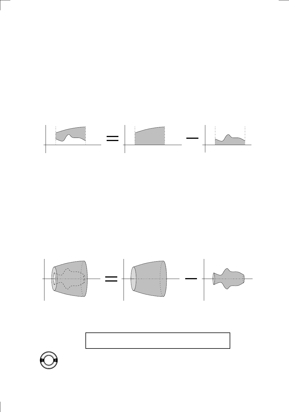
Section 29.1.5: Variation 2: regions between two curves • 625
29.1.5 Variation 2: regions between two curves
Suppose the region to be revolved lies between two curves. We’ll handle this
situation in the same way as finding the area of a region between two curves
in Section 16.4.2 of Chapter 16. The general idea is to take the top curve
and revolve the region under it all the way to the axis, to get a bigger solid
than you want. Now take the bottom curve and revolve the region under it
all the way to the axis, to get a solid which you actually need to cut out of
the big solid and throw away to get the desired solid. Finally, subtract the
small volume from the big one. Indeed, consider the following three regions:
PSfrag
replacements
(
a, b)
[
a, b]
(
a, b]
[
a, b)
(
a, ∞)
[
a, ∞)
(
−∞, b)
(
−∞, b]
(
−∞, ∞)
{
x : a < x < b}
{
x : a ≤ x ≤ b}
{
x : a < x ≤ b}
{
x : a ≤ x < b}
{
x : x ≥ a}
{
x : x > a}
{
x : x ≤ b}
{
x : x < b}
R
a
b
shado
w
0
1
4
−
2
3
−
3
g(
x) = x
2
f(
x) = x
3
g(
x) = x
2
f(
x) = x
3
mirror
(y = x)
f
−
1
(x) =
3
√
x
y = h
(x)
y = h
−
1
(x)
y =
(x − 1)
2
−
1
x
Same
height
−
x
Same
length,
opp
osite signs
y = −
2x
−
2
1
y =
1
2
x − 1
2
−
1
y =
2
x
y =
10
x
y =
2
−x
y =
log
2
(x)
4
3
units
mirror
(x-axis)
y = |
x|
y = |
log
2
(x)|
θ radians
θ units
30
◦
=
π
6
45
◦
=
π
4
60
◦
=
π
3
120
◦
=
2
π
3
135
◦
=
3
π
4
150
◦
=
5
π
6
90
◦
=
π
2
180
◦
= π
210
◦
=
7
π
6
225
◦
=
5
π
4
240
◦
=
4
π
3
270
◦
=
3
π
2
300
◦
=
5
π
3
315
◦
=
7
π
4
330
◦
=
11
π
6
0
◦
=
0 radians
θ
hypotenuse
opp
osite
adjacen
t
0
(≡ 2π)
π
2
π
3
π
2
I
I
I
I
II
IV
θ
(
x, y)
x
y
r
7
π
6
reference
angle
reference
angle =
π
6
sin
+
sin −
cos
+
cos −
tan
+
tan −
A
S
T
C
7
π
4
9
π
13
5
π
6
(this
angle is
5π
6
clo
ckwise)
1
2
1
2
3
4
5
6
0
−
1
−
2
−
3
−
4
−
5
−
6
−
3π
−
5
π
2
−
2π
−
3
π
2
−
π
−
π
2
3
π
3
π
5
π
2
2
π
3
π
2
π
π
2
y =
sin(x)
1
0
−
1
−
3π
−
5
π
2
−
2π
−
3
π
2
−
π
−
π
2
3
π
5
π
2
2
π
2
π
3
π
2
π
π
2
y =
sin(x)
y =
cos(x)
−
π
2
π
2
y =
tan(x), −
π
2
<
x <
π
2
0
−
π
2
π
2
y =
tan(x)
−
2π
−
3π
−
5
π
2
−
3
π
2
−
π
−
π
2
π
2
3
π
3
π
5
π
2
2
π
3
π
2
π
y =
sec(x)
y =
csc(x)
y =
cot(x)
y = f(
x)
−
1
1
2
y = g(
x)
3
y = h
(x)
4
5
−
2
f(
x) =
1
x
g(
x) =
1
x
2
etc.
0
1
π
1
2
π
1
3
π
1
4
π
1
5
π
1
6
π
1
7
π
g(
x) = sin
1
x
1
0
−
1
L
10
100
200
y =
π
2
y = −
π
2
y =
tan
−1
(x)
π
2
π
y =
sin
(x)
x
,
x > 3
0
1
−
1
a
L
f(
x) = x sin (1/x)
(0 <
x < 0.3)
h
(x) = x
g(
x) = −x
a
L
lim
x
→a
+
f(x) = L
lim
x
→a
+
f(x) = ∞
lim
x
→a
+
f(x) = −∞
lim
x
→a
+
f(x) DNE
lim
x
→a
−
f(x) = L
lim
x
→a
−
f(x) = ∞
lim
x
→a
−
f(x) = −∞
lim
x
→a
−
f(x) DNE
M
}
lim
x
→a
−
f(x) = M
lim
x
→a
f(x) = L
lim
x
→a
f(x) DNE
lim
x
→∞
f(x) = L
lim
x
→∞
f(x) = ∞
lim
x
→∞
f(x) = −∞
lim
x
→∞
f(x) DNE
lim
x
→−∞
f(x) = L
lim
x
→−∞
f(x) = ∞
lim
x
→−∞
f(x) = −∞
lim
x
→−∞
f(x) DNE
lim
x →a
+
f(
x) = ∞
lim
x →a
+
f(
x) = −∞
lim
x →a
−
f(
x) = ∞
lim
x →a
−
f(
x) = −∞
lim
x →a
f(
x) = ∞
lim
x →a
f(
x) = −∞
lim
x →a
f(
x) DNE
y = f (
x)
a
y =
|
x|
x
1
−
1
y =
|
x + 2|
x +
2
1
−
1
−
2
1
2
3
4
a
a
b
y = x sin
1
x
y = x
y = −
x
a
b
c
d
C
a
b
c
d
−
1
0
1
2
3
time
y
t
u
(
t, f(t))
(
u, f(u))
time
y
t
u
y
x
(
x, f(x))
y = |
x|
(
z, f(z))
z
y = f(
x)
a
tangen
t at x = a
b
tangen
t at x = b
c
tangen
t at x = c
y = x
2
tangen
t
at x = −
1
u
v
uv
u +
∆u
v +
∆v
(
u + ∆u)(v + ∆v)
∆
u
∆
v
u
∆v
v∆
u
∆
u∆v
y = f(
x)
1
2
−
2
y = |
x
2
− 4|
y = x
2
− 4
y = −
2x + 5
y = g(
x)
1
2
3
4
5
6
7
8
9
0
−
1
−
2
−
3
−
4
−
5
−
6
y = f (
x)
3
−
3
3
−
3
0
−
1
2
easy
hard
flat
y = f
0
(
x)
3
−
3
0
−
1
2
1
−
1
y =
sin(x)
y = x
x
A
B
O
1
C
D
sin(
x)
tan(
x)
y =
sin
(x)
x
π
2
π
1
−
1
x =
0
a =
0
x
> 0
a
> 0
x
< 0
a
< 0
rest
position
+
−
y = x
2
sin
1
x
N
A
B
H
a
b
c
O
H
A
B
C
D
h
r
R
θ
1000
2000
α
β
p
h
y = g(
x) = log
b
(x)
y = f (
x) = b
x
y = e
x
5
10
1
2
3
4
0
−
1
−
2
−
3
−
4
y =
ln(x)
y =
cosh(x)
y =
sinh(x)
y =
tanh(x)
y =
sech(x)
y =
csch(x)
y =
coth(x)
1
−
1
y = f(
x)
original
function
in
verse function
slop
e = 0 at (x, y)
slop
e is infinite at (y, x)
−
108
2
5
1
2
1
2
3
4
5
6
0
−
1
−
2
−
3
−
4
−
5
−
6
−
3π
−
5
π
2
−
2π
−
3
π
2
−
π
−
π
2
3
π
3
π
5
π
2
2
π
3
π
2
π
π
2
y =
sin(x)
1
0
−
1
−
3π
−
5
π
2
−
2π
−
3
π
2
−
π
−
π
2
3
π
5
π
2
2
π
2
π
3
π
2
π
π
2
y =
sin(x)
y =
sin(x), −
π
2
≤ x ≤
π
2
−
2
−
1
0
2
π
2
−
π
2
y =
sin
−1
(x)
y =
cos(x)
π
π
2
y =
cos
−1
(x)
−
π
2
1
x
α
β
y =
tan(x)
y =
tan(x)
1
y =
tan
−1
(x)
y =
sec(x)
y =
sec
−1
(x)
y =
csc
−1
(x)
y =
cot
−1
(x)
1
y =
cosh
−1
(x)
y =
sinh
−1
(x)
y =
tanh
−1
(x)
y =
sech
−1
(x)
y =
csch
−1
(x)
y =
coth
−1
(x)
(0
, 3)
(2
, −1)
(5
, 2)
(7
, 0)
(
−1, 44)
(0
, 1)
(1
, −12)
(2
, 305)
y =
1
2
(2
, 3)
y = f(
x)
y = g(
x)
a
b
c
a
b
c
s
c
0
c
1
(
a, f(a))
(
b, f(b))
1
2
1
2
3
4
5
6
0
−
1
−
2
−
3
−
4
−
5
−
6
−
3π
−
5
π
2
−
2π
−
3
π
2
−
π
−
π
2
3
π
3
π
5
π
2
2
π
3
π
2
π
π
2
y =
sin(x)
1
0
−
1
−
3π
−
5
π
2
−
2π
−
3
π
2
−
π
−
π
2
3
π
5
π
2
2
π
2
π
3
π
2
π
π
2
c
OR
Lo
cal maximum
Lo
cal minimum
Horizon
tal point of inflection
1
e
y = f
0
(
x)
y = f (
x) = x ln(x)
−
1
e
?
y = f (
x) = x
3
y = g(
x) = x
4
x
f(
x)
−
3
−
2
−
1
0
1
2
1
2
3
4
+
−
?
1
5
6
3
f
0
(
x)
2 −
1
2
√
6
2
+
1
2
√
6
f
00
(
x)
7
8
g
00
(
x)
f
00
(
x)
0
y =
(
x − 3)(x − 1)
2
x
3
(
x + 2)
y = x ln(
x)
1
e
−
1
e
5
−
108
2
α
β
2 −
1
2
√
6
2
+
1
2
√
6
y = x
2
(
x − 5)
3
−
e
−
1/2
√
3
e
−
1/2
√
3
−
e
−3/2
e
−
3/2
−
1
√
3
1
√
3
−
1
1
y = xe
−
3x
2
/2
y =
x
3
− 6
x
2
+ 13x −8
x
28
2
600
500
400
300
200
100
0
−
100
−
200
−
300
−
400
−
500
−
600
0
10
−
10
5
−
5
20
−
20
15
−
15
0
4
5
6
x
P
0
(
x)
+
−
−
existing
fence
new
fence
enclosure
A
h
b
H
99
100
101
h
dA/dh
r
h
1
2
7
shallo
w
deep
LAND
SEA
N
y
z
s
t
3
11
9
L
(11)
√
11
y = L
(x)
y = f (
x)
11
y = L
(x)
y = f(
x)
F
P
a
a +
∆x
f(
a + ∆x)
L
(a + ∆x)
f(
a)
error
d
f
∆
x
a
b
y = f(
x)
true
zero
starting
approximation
b
etter approximation
v
t
3
5
50
40
60
4
20
30
25
t
1
t
2
t
3
t
4
t
n
−2
t
n
−1
t
0
= a
t
n
= b
v
1
v
2
v
3
v
4
v
n
−1
v
n
−
30
6
30
|
v|
a
b
p
q
c
v(
c)
v(
c
1
)
v(
c
2
)
v(
c
3
)
v(
c
4
)
v(
c
5
)
v(
c
6
)
t
1
t
2
t
3
t
4
t
5
c
1
c
2
c
3
c
4
c
5
c
6
t
0
=
a
t
6
=
b
t
16
=
b
t
10
=
b
a
b
x
y
y = f(
x)
1
2
y = x
5
0
−
2
y =
1
a
b
y =
sin(x)
π
−
π
0
−
1
−
2
0
2
4
y = x
2
0
1
2
3
4
2
n
4
n
6
n
2(
n−2)
n
2(
n−1)
n
2
n
n
=
2
width
of each interval =
2
n
−
2
1
3
0
I
I
I
I
II
IV
4
y
dx
y = −
x
2
− 2x + 3
3
−
5
y = |−
x
2
− 2x + 3|
I
I
I
I
Ia
5
3
0
1
2
a
b
y = f (
x)
y = g(
x)
y = x
2
a
b
5
3
0
1
2
y =
√
x
2
√
2
2
2
dy
x
2
a
b
y = f(
x)
y = g(
x)
M
m
1
2
−
1
−
2
0
y = e
−
x
2
1
2
e
−
1/4
f
a
v
y = f
a
v
c
A
M
0
1
2
a
b
x
t
y = f (
t)
F (
x )
y = f (
t)
F (
x + h )
x + h
F (
x + h) − F (x)
f(
x)
1
2
y =
sin(x)
π
−
π
−
1
−
2
y =
1
x
y = x
2
1
2
1
−
1
y =
ln|x|
θ
a
x
a
x
p
a
2
− x
2
3
x
p
9 − x
2
p
x
2
+ a
2
x
a
p
x
2
+ 15
x
√
15
x
p
x
2
− a
2
a
x
p
x
2
− 4
2
x
−
p
x
2
− a
2
a
x
−
p
x
2
− 4
2
y = f(
x)
a
b
a + ε
ε
Z
b
a
+ε
f(x) dx
small
ev
en smaller
y = g(
x)
infinite
area
finite
area
1
y =
1
x
y =
1
x
p
, p
< 1 (typical)
y =
1
x
p
, p
> 1 (typical)
a
1
a
2
a
3
a
4
a
5
a
6
a
7
a
8
1
2
3
4
5
6
7
8
n
a
n
x
y
y = f(
x)
(
a, f(a))
a
−
1
0
1
a
6
1
2
7
1
2
7
?
−
2
−
1
−
2
t =
0
t = π
/6
t = π
/4
t = π
/3
t = π
/2
3
0
t = −
2
t = −
3/2
t = ±
1
t = −
1/2
t =
0
t =
1/2
t =
3/2
t =
2
12
−
12
θ
r
P
θ
r
P
11
π
6
2
(
−1, −1)
wrong
point
π
4
5
π
4
√
2
(0
, 1)
(0
, −3)
(
−2, 0)
π
2
3
π
2
π
r =
3 sin(θ)
3
π
2
θ
2
π
1
0
−
1
−
2
−
3
0
3
2
−
3
2
0
r =
1 + 2 cos(θ)
2
π
3
4
π
3
0
π
0
pi
−
3
2
3
π
2
1
2
3
0
−
1
−
2
−
3
0 ≤ θ ≤
2
π
3
0 ≤ θ ≤ π
0 ≤ θ ≤ 2π
r = 1 + cos(θ)
r = 1 +
3
4
cos(θ)
−
1
4
r = sin(2θ)
r = sin(3θ)
r =
1
π
θ
0 ≤ θ ≤ 4π
r =
2
1 + sin(θ)
−
π
4
≤ θ ≤
5π
4
0 ≤ θ ≤ 2π
0 ≤ θ ≤ π
−4
−5
4
5
f(θ)
f(θ + dθ)
θ
dθ
θ + dθ
approximating region
exact region
0 ≤ θ ≤ 2π
r = |1 + 2 cos(θ)|
2i
2 − 3i
−1
θ = 0
θ =
π
4
θ =
π
2
θ =
2π
3
θ = π
θ =
13π
12
θ =
3π
2
θ =
7π
4
1 = e
0
e
i
π
4
i = e
i
π
2
e
i
2π
3
−1 = e
iπ
e
i
13π
12
−i = e
i
3π
2
e
i
7π
4
i
−i
1
θ
1 − i
2i
−2i
2
−2
6i
−6i
6
−6
−
√
3
R
ϕ
2
1/5
θ =
π
6
θ =
17π
30
θ =
29π
30
θ =
41π
30
θ =
53π
30
z
0
z
1
z
2
z
3
z
4
−
√
3
2
√
3
2
1
2
i
−i
19π
6
−i
7π
6
i
5π
6
i
17π
6
i
29π
6
ln(2)
−
7π
4
−
3π
4
π
4
5π
4
9π
4
3
2
i
0
1
2
3
4
dx
y
x
y =
p
1 − (x − 3)
2
2πx
a
b
y = f(x)
A
B
y =
√
x
1
The region we want to revolve is shown in the left-hand picture; it is the set
difference of the region under the top curve down to the x-axis (in the middle
picture above) and the region under the bottom curve down to the x-axis
(in the right-hand picture). Now, regardless of whether you revolve about
the x-axis or the y-axis, the volume of revolution of the region we want is
equal to the difference between the volume of revolution of the big region and
the volume of revolution of the small region. For example, if you revolve the
region about the x-axis, then you get a cone-like structure with chopped-off
ends and a weird-shaped hole going through the middle of it from left to right.
The solid is the set difference of the filled-in version (with no hole) and the
hole itself:
PSfrag
replacements
(
a, b)
[
a, b]
(
a, b]
[
a, b)
(
a, ∞)
[
a, ∞)
(
−∞, b)
(
−∞, b]
(
−∞, ∞)
{
x : a < x < b}
{
x : a ≤ x ≤ b}
{
x : a < x ≤ b}
{
x : a ≤ x < b}
{
x : x ≥ a}
{
x : x > a}
{
x : x ≤ b}
{
x : x < b}
R
a
b
shado
w
0
1
4
−
2
3
−
3
g(
x) = x
2
f(
x) = x
3
g(
x) = x
2
f(
x) = x
3
mirror
(y = x)
f
−
1
(x) =
3
√
x
y = h
(x)
y = h
−
1
(x)
y =
(x − 1)
2
−
1
x
Same
height
−
x
Same
length,
opp
osite signs
y = −
2x
−
2
1
y =
1
2
x − 1
2
−
1
y =
2
x
y =
10
x
y =
2
−x
y =
log
2
(x)
4
3
units
mirror
(x-axis)
y = |
x|
y = |
log
2
(x)|
θ radians
θ units
30
◦
=
π
6
45
◦
=
π
4
60
◦
=
π
3
120
◦
=
2
π
3
135
◦
=
3
π
4
150
◦
=
5
π
6
90
◦
=
π
2
180
◦
= π
210
◦
=
7
π
6
225
◦
=
5
π
4
240
◦
=
4
π
3
270
◦
=
3
π
2
300
◦
=
5
π
3
315
◦
=
7
π
4
330
◦
=
11
π
6
0
◦
=
0 radians
θ
hypotenuse
opp
osite
adjacen
t
0
(≡ 2π)
π
2
π
3
π
2
I
I
I
I
II
IV
θ
(
x, y)
x
y
r
7
π
6
reference
angle
reference
angle =
π
6
sin
+
sin −
cos
+
cos −
tan
+
tan −
A
S
T
C
7
π
4
9
π
13
5
π
6
(this
angle is
5π
6
clo
ckwise)
1
2
1
2
3
4
5
6
0
−
1
−
2
−
3
−
4
−
5
−
6
−
3π
−
5
π
2
−
2π
−
3
π
2
−
π
−
π
2
3
π
3
π
5
π
2
2
π
3
π
2
π
π
2
y =
sin(x)
1
0
−
1
−
3π
−
5
π
2
−
2π
−
3
π
2
−
π
−
π
2
3
π
5
π
2
2
π
2
π
3
π
2
π
π
2
y =
sin(x)
y =
cos(x)
−
π
2
π
2
y =
tan(x), −
π
2
<
x <
π
2
0
−
π
2
π
2
y =
tan(x)
−
2π
−
3π
−
5
π
2
−
3
π
2
−
π
−
π
2
π
2
3
π
3
π
5
π
2
2
π
3
π
2
π
y =
sec(x)
y =
csc(x)
y =
cot(x)
y = f (
x)
−
1
1
2
y = g(
x)
3
y = h
(x)
4
5
−
2
f(
x) =
1
x
g(
x) =
1
x
2
etc.
0
1
π
1
2
π
1
3
π
1
4
π
1
5
π
1
6
π
1
7
π
g(
x) = sin
1
x
1
0
−
1
L
10
100
200
y =
π
2
y = −
π
2
y =
tan
−1
(x)
π
2
π
y =
sin(
x)
x
,
x > 3
0
1
−
1
a
L
f(
x) = x sin (1/x)
(0 <
x < 0.3)
h
(x) = x
g(
x) = −x
a
L
lim
x
→a
+
f(x) = L
lim
x
→a
+
f(x) = ∞
lim
x
→a
+
f(x) = −∞
lim
x
→a
+
f(x) DNE
lim
x
→a
−
f(x) = L
lim
x
→a
−
f(x) = ∞
lim
x
→a
−
f(x) = −∞
lim
x
→a
−
f(x) DNE
M
}
lim
x
→a
−
f(x) = M
lim
x
→a
f(x) = L
lim
x
→a
f(x) DNE
lim
x
→∞
f(x) = L
lim
x
→∞
f(x) = ∞
lim
x
→∞
f(x) = −∞
lim
x
→∞
f(x) DNE
lim
x
→−∞
f(x) = L
lim
x
→−∞
f(x) = ∞
lim
x
→−∞
f(x) = −∞
lim
x
→−∞
f(x) DNE
lim
x →a
+
f(
x) = ∞
lim
x →a
+
f(
x) = −∞
lim
x →a
−
f(
x) = ∞
lim
x →a
−
f(
x) = −∞
lim
x →a
f(
x) = ∞
lim
x →a
f(
x) = −∞
lim
x →a
f(
x) DNE
y = f (
x)
a
y =
|
x|
x
1
−
1
y =
|
x + 2|
x +
2
1
−
1
−
2
1
2
3
4
a
a
b
y = x sin
1
x
y = x
y = −
x
a
b
c
d
C
a
b
c
d
−
1
0
1
2
3
time
y
t
u
(
t, f(t))
(
u, f(u))
time
y
t
u
y
x
(
x, f(x))
y = |
x|
(
z, f(z))
z
y = f (
x)
a
tangen
t at x = a
b
tangen
t at x = b
c
tangen
t at x = c
y = x
2
tangen
t
at x = −
1
u
v
uv
u +
∆u
v +
∆v
(
u + ∆u)(v + ∆v)
∆
u
∆
v
u
∆v
v∆
u
∆
u∆v
y = f (
x)
1
2
−
2
y = |
x
2
− 4|
y = x
2
− 4
y = −
2x + 5
y = g(
x)
1
2
3
4
5
6
7
8
9
0
−
1
−
2
−
3
−
4
−
5
−
6
y = f (
x)
3
−
3
3
−
3
0
−
1
2
easy
hard
flat
y = f
0
(
x)
3
−
3
0
−
1
2
1
−
1
y =
sin(x)
y = x
x
A
B
O
1
C
D
sin(
x)
tan(
x)
y =
sin
(x)
x
π
2
π
1
−
1
x =
0
a =
0
x
> 0
a
> 0
x
< 0
a
< 0
rest
position
+
−
y = x
2
sin
1
x
N
A
B
H
a
b
c
O
H
A
B
C
D
h
r
R
θ
1000
2000
α
β
p
h
y = g(
x) = log
b
(x)
y = f (
x) = b
x
y = e
x
5
10
1
2
3
4
0
−
1
−
2
−
3
−
4
y =
ln(x)
y =
cosh(x)
y =
sinh(x)
y =
tanh(x)
y =
sech(x)
y =
csch(x)
y =
coth(x)
1
−
1
y = f (
x)
original
function
in
verse function
slop
e = 0 at (x, y)
slop
e is infinite at (y, x)
−
108
2
5
1
2
1
2
3
4
5
6
0
−
1
−
2
−
3
−
4
−
5
−
6
−
3π
−
5
π
2
−
2π
−
3
π
2
−
π
−
π
2
3
π
3
π
5
π
2
2
π
3
π
2
π
π
2
y =
sin(x)
1
0
−
1
−
3π
−
5
π
2
−
2π
−
3
π
2
−
π
−
π
2
3
π
5
π
2
2
π
2
π
3
π
2
π
π
2
y =
sin(x)
y =
sin(x), −
π
2
≤ x ≤
π
2
−
2
−
1
0
2
π
2
−
π
2
y =
sin
−1
(x)
y =
cos(x)
π
π
2
y =
cos
−1
(x)
−
π
2
1
x
α
β
y =
tan(x)
y =
tan(x)
1
y =
tan
−1
(x)
y =
sec(x)
y =
sec
−1
(x)
y =
csc
−1
(x)
y =
cot
−1
(x)
1
y =
cosh
−1
(x)
y =
sinh
−1
(x)
y =
tanh
−1
(x)
y =
sech
−1
(x)
y =
csch
−1
(x)
y =
coth
−1
(x)
(0
, 3)
(2
, −1)
(5
, 2)
(7
, 0)
(
−1, 44)
(0
, 1)
(1
, −12)
(2
, 305)
y =
1
2
(2
, 3)
y = f (
x)
y = g(
x)
a
b
c
a
b
c
s
c
0
c
1
(
a, f(a))
(
b, f(b))
1
2
1
2
3
4
5
6
0
−
1
−
2
−
3
−
4
−
5
−
6
−
3π
−
5
π
2
−
2π
−
3
π
2
−
π
−
π
2
3
π
3
π
5
π
2
2
π
3
π
2
π
π
2
y =
sin(x)
1
0
−
1
−
3π
−
5
π
2
−
2π
−
3
π
2
−
π
−
π
2
3
π
5
π
2
2
π
2
π
3
π
2
π
π
2
c
OR
Lo
cal maximum
Lo
cal minimum
Horizon
tal point of inflection
1
e
y = f
0
(
x)
y = f (
x) = x ln(x)
−
1
e
?
y = f (
x) = x
3
y = g(
x) = x
4
x
f(
x)
−
3
−
2
−
1
0
1
2
1
2
3
4
+
−
?
1
5
6
3
f
0
(
x)
2 −
1
2
√
6
2
+
1
2
√
6
f
00
(
x)
7
8
g
00
(
x)
f
00
(
x)
0
y =
(
x − 3)(x − 1)
2
x
3
(
x + 2)
y = x ln
(x)
1
e
−
1
e
5
−
108
2
α
β
2 −
1
2
√
6
2
+
1
2
√
6
y = x
2
(
x − 5)
3
−
e
−
1/2
√
3
e
−
1/2
√
3
−
e
−3/2
e
−
3/2
−
1
√
3
1
√
3
−
1
1
y = xe
−
3x
2
/2
y =
x
3
− 6
x
2
+ 13x −8
x
28
2
600
500
400
300
200
100
0
−
100
−
200
−
300
−
400
−
500
−
600
0
10
−
10
5
−
5
20
−
20
15
−
15
0
4
5
6
x
P
0
(
x)
+
−
−
existing
fence
new
fence
enclosure
A
h
b
H
99
100
101
h
dA/dh
r
h
1
2
7
shallo
w
deep
LAND
SEA
N
y
z
s
t
3
11
9
L
(11)
√
11
y = L
(x)
y = f (
x)
11
y = L
(x)
y = f (
x)
F
P
a
a +
∆x
f(
a + ∆x)
L
(a + ∆x)
f(
a)
error
d
f
∆
x
a
b
y = f (
x)
true
zero
starting
approximation
b
etter approximation
v
t
3
5
50
40
60
4
20
30
25
t
1
t
2
t
3
t
4
t
n
−2
t
n
−1
t
0
= a
t
n
= b
v
1
v
2
v
3
v
4
v
n
−1
v
n
−
30
6
30
|
v|
a
b
p
q
c
v(
c)
v(
c
1
)
v(
c
2
)
v(
c
3
)
v(
c
4
)
v(
c
5
)
v(
c
6
)
t
1
t
2
t
3
t
4
t
5
c
1
c
2
c
3
c
4
c
5
c
6
t
0
=
a
t
6
=
b
t
16
=
b
t
10
=
b
a
b
x
y
y = f (
x)
1
2
y = x
5
0
−
2
y =
1
a
b
y =
sin(x)
π
−
π
0
−
1
−
2
0
2
4
y = x
2
0
1
2
3
4
2
n
4
n
6
n
2(
n−2)
n
2(
n−1)
n
2
n
n
=
2
width
of each interval =
2
n
−
2
1
3
0
I
I
I
I
II
IV
4
y
dx
y = −
x
2
− 2x + 3
3
−
5
y = |−
x
2
− 2x + 3|
I
I
I
I
Ia
5
3
0
1
2
a
b
y = f (
x)
y = g(
x)
y = x
2
a
b
5
3
0
1
2
y =
√
x
2
√
2
2
2
dy
x
2
a
b
y = f (
x)
y = g(
x)
M
m
1
2
−
1
−
2
0
y = e
−
x
2
1
2
e
−
1/4
f
a
v
y = f
a
v
c
A
M
0
1
2
a
b
x
t
y = f (
t)
F (
x )
y = f(
t)
F (
x + h )
x + h
F (
x + h) − F (x)
f(
x)
1
2
y =
sin(x)
π
−
π
−
1
−
2
y =
1
x
y = x
2
1
2
1
−
1
y =
ln|x|
θ
a
x
a
x
p
a
2
− x
2
3
x
p
9 − x
2
p
x
2
+ a
2
x
a
p
x
2
+ 15
x
√
15
x
p
x
2
− a
2
a
x
p
x
2
− 4
2
x
−
p
x
2
− a
2
a
x
−
p
x
2
− 4
2
y = f (
x)
a
b
a + ε
ε
Z
b
a
+ε
f(x) dx
small
ev
en smaller
y = g(
x)
infinite
area
finite
area
1
y =
1
x
y =
1
x
p
, p
< 1 (typical)
y =
1
x
p
, p
> 1 (typical)
a
1
a
2
a
3
a
4
a
5
a
6
a
7
a
8
1
2
3
4
5
6
7
8
n
a
n
x
y
y = f (
x)
(
a, f(a))
a
−
1
0
1
a
6
1
2
7
1
2
7
?
−
2
−
1
−
2
t =
0
t = π
/6
t = π
/4
t = π
/3
t = π
/2
3
0
t = −
2
t = −
3/2
t = ±
1
t = −
1/2
t =
0
t =
1/2
t =
3/2
t =
2
12
−
12
θ
r
P
θ
r
P
11
π
6
2
(
−1, −1)
wrong
point
π
4
5
π
4
√
2
(0
, 1)
(0
, −3)
(
−2, 0)
π
2
3
π
2
π
r =
3 sin(θ)
3
π
2
θ
2π
1
0
−1
−2
−3
0
3
2
−
3
2
0
r = 1 + 2 cos(θ)
2π
3
4π
3
0
π
0
pi
−
3
2
3π
2
1
2
3
0
−1
−2
−3
0 ≤ θ ≤
2π
3
0 ≤ θ ≤ π
0 ≤ θ ≤ 2π
r = 1 + cos(θ)
r = 1 +
3
4
cos(θ)
−
1
4
r = sin(2θ)
r = sin(3θ)
r =
1
π
θ
0 ≤ θ ≤ 4π
r =
2
1 + sin(θ)
−
π
4
≤ θ ≤
5π
4
0 ≤ θ ≤ 2π
0 ≤ θ ≤ π
−4
−5
4
5
f(θ)
f(θ + dθ)
θ
dθ
θ + dθ
approximating region
exact region
0 ≤ θ ≤ 2π
r = |1 + 2 cos(θ)|
2i
2 − 3i
−1
θ = 0
θ =
π
4
θ =
π
2
θ =
2π
3
θ = π
θ =
13π
12
θ =
3π
2
θ =
7π
4
1 = e
0
e
i
π
4
i = e
i
π
2
e
i
2π
3
−1 = e
iπ
e
i
13π
12
−i = e
i
3π
2
e
i
7π
4
i
−i
1
θ
1 − i
2i
−2i
2
−2
6i
−6i
6
−6
−
√
3
R
ϕ
2
1/5
θ =
π
6
θ =
17π
30
θ =
29π
30
θ =
41π
30
θ =
53π
30
z
0
z
1
z
2
z
3
z
4
−
√
3
2
√
3
2
1
2
i
−i
19π
6
−i
7π
6
i
5π
6
i
17π
6
i
29π
6
ln(2)
−
7π
4
−
3π
4
π
4
5π
4
9π
4
3
2
i
0
1
2
3
4
dx
y
x
y =
p
1 − (x − 3)
2
2πx
a
b
y = f (x)
A
B
y =
√
x
1
So, here’s what we conclude:
If the region lies between two curves, find the difference
between the two corresponding volumes of revolution.
Let’s look at a concrete example. Consider the finite region between the curves
PSfrag
replacements
(
a, b)
[
a, b]
(
a, b]
[
a, b)
(
a, ∞)
[
a, ∞)
(
−∞, b)
(
−∞, b]
(
−∞, ∞)
{
x : a < x < b}
{
x : a ≤ x ≤ b}
{
x : a < x ≤ b}
{
x : a ≤ x < b}
{
x : x ≥ a}
{
x : x > a}
{
x : x ≤ b}
{
x : x < b}
R
a
b
shado
w
0
1
4
−
2
3
−
3
g(
x) = x
2
f(
x) = x
3
g(
x) = x
2
f(
x) = x
3
mirror
(y = x)
f
−
1
(x) =
3
√
x
y = h
(x)
y = h
−
1
(x)
y =
(x − 1)
2
−
1
x
Same
height
−
x
Same
length,
opp
osite signs
y = −
2x
−
2
1
y =
1
2
x − 1
2
−
1
y =
2
x
y =
10
x
y =
2
−x
y =
log
2
(x)
4
3
units
mirror
(x-axis)
y = |
x|
y = |
log
2
(x)|
θ radians
θ units
30
◦
=
π
6
45
◦
=
π
4
60
◦
=
π
3
120
◦
=
2
π
3
135
◦
=
3
π
4
150
◦
=
5
π
6
90
◦
=
π
2
180
◦
= π
210
◦
=
7
π
6
225
◦
=
5
π
4
240
◦
=
4
π
3
270
◦
=
3
π
2
300
◦
=
5
π
3
315
◦
=
7
π
4
330
◦
=
11
π
6
0
◦
=
0 radians
θ
hyp
otenuse
opp
osite
adjacen
t
0
(≡ 2π)
π
2
π
3
π
2
I
I
I
I
II
IV
θ
(
x, y)
x
y
r
7
π
6
reference
angle
reference
angle =
π
6
sin
+
sin −
cos
+
cos −
tan
+
tan −
A
S
T
C
7
π
4
9
π
13
5
π
6
(this
angle is
5π
6
clo
ckwise)
1
2
1
2
3
4
5
6
0
−
1
−
2
−
3
−
4
−
5
−
6
−
3π
−
5
π
2
−
2π
−
3
π
2
−
π
−
π
2
3
π
3
π
5
π
2
2
π
3
π
2
π
π
2
y =
sin(x)
1
0
−
1
−
3π
−
5
π
2
−
2π
−
3
π
2
−
π
−
π
2
3
π
5
π
2
2
π
2
π
3
π
2
π
π
2
y =
sin(x)
y =
cos(x)
−
π
2
π
2
y =
tan(x), −
π
2
<
x <
π
2
0
−
π
2
π
2
y =
tan(x)
−
2π
−
3π
−
5
π
2
−
3
π
2
−
π
−
π
2
π
2
3
π
3
π
5
π
2
2
π
3
π
2
π
y =
sec(x)
y =
csc(x)
y =
cot(x)
y = f(
x)
−
1
1
2
y = g(
x)
3
y = h
(x)
4
5
−
2
f(
x) =
1
x
g(
x) =
1
x
2
etc.
0
1
π
1
2
π
1
3
π
1
4
π
1
5
π
1
6
π
1
7
π
g(
x) = sin
1
x
1
0
−
1
L
10
100
200
y =
π
2
y = −
π
2
y =
tan
−1
(x)
π
2
π
y =
sin(
x)
x
,
x > 3
0
1
−
1
a
L
f(
x) = x sin (1/x)
(0 <
x < 0.3)
h
(x) = x
g(
x) = −x
a
L
lim
x
→a
+
f(x) = L
lim
x
→a
+
f(x) = ∞
lim
x
→a
+
f(x) = −∞
lim
x
→a
+
f(x) DNE
lim
x
→a
−
f(x) = L
lim
x
→a
−
f(x) = ∞
lim
x
→a
−
f(x) = −∞
lim
x
→a
−
f(x) DNE
M
}
lim
x
→a
−
f(x) = M
lim
x
→a
f(x) = L
lim
x
→a
f(x) DNE
lim
x
→∞
f(x) = L
lim
x
→∞
f(x) = ∞
lim
x
→∞
f(x) = −∞
lim
x
→∞
f(x) DNE
lim
x
→−∞
f(x) = L
lim
x
→−∞
f(x) = ∞
lim
x
→−∞
f(x) = −∞
lim
x
→−∞
f(x) DNE
lim
x →a
+
f(
x) = ∞
lim
x →a
+
f(
x) = −∞
lim
x →a
−
f(
x) = ∞
lim
x →a
−
f(
x) = −∞
lim
x →a
f(
x) = ∞
lim
x →a
f(
x) = −∞
lim
x →a
f(
x) DNE
y = f (
x)
a
y =
|
x|
x
1
−
1
y =
|
x + 2|
x +
2
1
−
1
−
2
1
2
3
4
a
a
b
y = x sin
1
x
y = x
y = −
x
a
b
c
d
C
a
b
c
d
−
1
0
1
2
3
time
y
t
u
(
t, f(t))
(
u, f(u))
time
y
t
u
y
x
(
x, f(x))
y = |
x|
(
z, f(z))
z
y = f(
x)
a
tangen
t at x = a
b
tangen
t at x = b
c
tangen
t at x = c
y = x
2
tangen
t
at x = −
1
u
v
uv
u +
∆u
v +
∆v
(
u + ∆u)(v + ∆v)
∆
u
∆
v
u
∆v
v∆
u
∆
u∆v
y = f(
x)
1
2
−
2
y = |
x
2
− 4|
y = x
2
− 4
y = −
2x + 5
y = g(
x)
1
2
3
4
5
6
7
8
9
0
−
1
−
2
−
3
−
4
−
5
−
6
y = f (
x)
3
−
3
3
−
3
0
−
1
2
easy
hard
flat
y = f
0
(
x)
3
−
3
0
−
1
2
1
−
1
y =
sin(x)
y = x
x
A
B
O
1
C
D
sin(
x)
tan(
x)
y =
sin(
x)
x
π
2
π
1
−
1
x =
0
a =
0
x
> 0
a
> 0
x
< 0
a
< 0
rest
position
+
−
y = x
2
sin
1
x
N
A
B
H
a
b
c
O
H
A
B
C
D
h
r
R
θ
1000
2000
α
β
p
h
y = g(
x) = log
b
(x)
y = f(
x) = b
x
y = e
x
5
10
1
2
3
4
0
−
1
−
2
−
3
−
4
y =
ln(x)
y =
cosh(x)
y =
sinh(x)
y =
tanh(x)
y =
sech(x)
y =
csch(x)
y =
coth(x)
1
−
1
y = f(
x)
original
function
in
verse function
slop
e = 0 at (x, y)
slop
e is infinite at (y, x)
−
108
2
5
1
2
1
2
3
4
5
6
0
−
1
−
2
−
3
−
4
−
5
−
6
−
3π
−
5
π
2
−
2π
−
3
π
2
−
π
−
π
2
3
π
3
π
5
π
2
2
π
3
π
2
π
π
2
y =
sin(x)
1
0
−
1
−
3π
−
5
π
2
−
2π
−
3
π
2
−
π
−
π
2
3
π
5
π
2
2
π
2
π
3
π
2
π
π
2
y =
sin(x)
y =
sin(x), −
π
2
≤ x ≤
π
2
−
2
−
1
0
2
π
2
−
π
2
y =
sin
−1
(x)
y =
cos(x)
π
π
2
y =
cos
−1
(x)
−
π
2
1
x
α
β
y =
tan(x)
y =
tan(x)
1
y =
tan
−1
(x)
y =
sec(x)
y =
sec
−1
(x)
y =
csc
−1
(x)
y =
cot
−1
(x)
1
y =
cosh
−1
(x)
y =
sinh
−1
(x)
y =
tanh
−1
(x)
y =
sech
−1
(x)
y =
csch
−1
(x)
y =
coth
−1
(x)
(0
, 3)
(2
, −1)
(5
, 2)
(7
, 0)
(
−1, 44)
(0
, 1)
(1
, −12)
(2
, 305)
y =
1
2
(2
, 3)
y = f(
x)
y = g(
x)
a
b
c
a
b
c
s
c
0
c
1
(
a, f(a))
(
b, f(b))
1
2
1
2
3
4
5
6
0
−
1
−
2
−
3
−
4
−
5
−
6
−
3π
−
5
π
2
−
2π
−
3
π
2
−
π
−
π
2
3
π
3
π
5
π
2
2
π
3
π
2
π
π
2
y =
sin(x)
1
0
−
1
−
3π
−
5
π
2
−
2π
−
3
π
2
−
π
−
π
2
3
π
5
π
2
2
π
2
π
3
π
2
π
π
2
c
OR
Lo
cal maximum
Lo
cal minimum
Horizon
tal point of inflection
1
e
y = f
0
(
x)
y = f (
x) = x ln(x)
−
1
e
?
y = f(
x) = x
3
y = g(
x) = x
4
x
f(
x)
−
3
−
2
−
1
0
1
2
1
2
3
4
+
−
?
1
5
6
3
f
0
(
x)
2 −
1
2
√
6
2
+
1
2
√
6
f
00
(
x)
7
8
g
00
(
x)
f
00
(
x)
0
y =
(
x − 3)(x − 1)
2
x
3
(
x + 2)
y = x ln
(x)
1
e
−
1
e
5
−
108
2
α
β
2 −
1
2
√
6
2
+
1
2
√
6
y = x
2
(
x − 5)
3
−
e
−
1/2
√
3
e
−
1/2
√
3
−
e
−3/2
e
−
3/2
−
1
√
3
1
√
3
−
1
1
y = xe
−
3x
2
/2
y =
x
3
− 6
x
2
+ 13x − 8
x
28
2
600
500
400
300
200
100
0
−
100
−
200
−
300
−
400
−
500
−
600
0
10
−
10
5
−
5
20
−
20
15
−
15
0
4
5
6
x
P
0
(
x)
+
−
−
existing
fence
new
fence
enclosure
A
h
b
H
99
100
101
h
dA/dh
r
h
1
2
7
shallo
w
deep
LAND
SEA
N
y
z
s
t
3
11
9
L
(11)
√
11
y = L
(x)
y = f (
x)
11
y = L
(x)
y = f(
x)
F
P
a
a +
∆x
f(
a + ∆x)
L
(a + ∆x)
f(
a)
error
d
f
∆
x
a
b
y = f(
x)
true
zero
starting
approximation
b
etter approximation
v
t
3
5
50
40
60
4
20
30
25
t
1
t
2
t
3
t
4
t
n
−2
t
n
−1
t
0
= a
t
n
= b
v
1
v
2
v
3
v
4
v
n
−1
v
n
−
30
6
30
|
v|
a
b
p
q
c
v(
c)
v(
c
1
)
v(
c
2
)
v(
c
3
)
v(
c
4
)
v(
c
5
)
v(
c
6
)
t
1
t
2
t
3
t
4
t
5
c
1
c
2
c
3
c
4
c
5
c
6
t
0
=
a
t
6
=
b
t
16
=
b
t
10
=
b
a
b
x
y
y = f(
x)
1
2
y = x
5
0
−
2
y =
1
a
b
y =
sin(x)
π
−
π
0
−
1
−
2
0
2
4
y = x
2
0
1
2
3
4
2
n
4
n
6
n
2(
n−2)
n
2(
n−1)
n
2
n
n
=
2
width
of each interval =
2
n
−
2
1
3
0
I
I
I
I
II
IV
4
y
dx
y = −
x
2
− 2x + 3
3
−
5
y = |−
x
2
− 2x + 3|
I
I
I
I
Ia
5
3
0
1
2
a
b
y = f (
x)
y = g(
x)
y = x
2
a
b
5
3
0
1
2
y =
√
x
2
√
2
2
2
dy
x
2
a
b
y = f(
x)
y = g(
x)
M
m
1
2
−
1
−
2
0
y = e
−
x
2
1
2
e
−
1/4
f
a
v
y = f
a
v
c
A
M
0
1
2
a
b
x
t
y = f (
t)
F (
x )
y = f (
t)
F (
x + h)
x + h
F (
x + h) − F (x)
f(
x)
1
2
y =
sin(x)
π
−
π
−
1
−
2
y =
1
x
y = x
2
1
2
1
−
1
y =
ln|x|
θ
a
x
a
x
p
a
2
− x
2
3
x
p
9 − x
2
p
x
2
+ a
2
x
a
p
x
2
+ 15
x
√
15
x
p
x
2
− a
2
a
x
p
x
2
− 4
2
x
−
p
x
2
− a
2
a
x
−
p
x
2
− 4
2
y = f(
x)
a
b
a + ε
ε
Z
b
a
+ε
f(x) dx
small
ev
en smaller
y = g(
x)
infinite
area
finite
area
1
y =
1
x
y =
1
x
p
, p
< 1 (typical)
y =
1
x
p
, p
> 1 (typical)
a
1
a
2
a
3
a
4
a
5
a
6
a
7
a
8
1
2
3
4
5
6
7
8
n
a
n
x
y
y = f(
x)
(
a, f(a))
a
−
1
0
1
a
6
1
2
7
1
2
7
?
−
2
−
1
−
2
t =
0
t = π
/6
t = π
/4
t = π
/3
t = π
/2
3
0
t = −
2
t = −
3/2
t = ±
1
t = −
1/2
t =
0
t =
1/2
t =
3/2
t =
2
12
−
12
θ
r
P
θ
r
P
11
π
6
2
(
−1, −1)
wrong
point
π
4
5
π
4
√
2
(0
, 1)
(0
, −3)
(
−2, 0)
π
2
3
π
2
π
r =
3 sin(θ)
3
π
2
θ
2
π
1
0
−
1
−
2
−
3
0
3
2
−
3
2
0
r =
1 + 2 cos(θ)
2
π
3
4
π
3
0
π
0
pi
−
3
2
3
π
2
1
2
3
0
−1
−2
−3
0 ≤ θ ≤
2π
3
0 ≤ θ ≤ π
0 ≤ θ ≤ 2π
r = 1 + cos(θ)
r = 1 +
3
4
cos(θ)
−
1
4
r = sin(2θ)
r = sin(3θ)
r =
1
π
θ
0 ≤ θ ≤ 4π
r =
2
1 + sin(θ)
−
π
4
≤ θ ≤
5π
4
0 ≤ θ ≤ 2π
0 ≤ θ ≤ π
−4
−5
4
5
f(θ)
f(θ + dθ)
θ
dθ
θ + dθ
approximating region
exact region
0 ≤ θ ≤ 2π
r = |1 + 2 cos(θ)|
2i
2 − 3i
−1
θ = 0
θ =
π
4
θ =
π
2
θ =
2π
3
θ = π
θ =
13π
12
θ =
3π
2
θ =
7π
4
1 = e
0
e
i
π
4
i = e
i
π
2
e
i
2π
3
−1 = e
iπ
e
i
13π
12
−i = e
i
3π
2
e
i
7π
4
i
−i
1
θ
1 − i
2i
−2i
2
−2
6i
−6i
6
−6
−
√
3
R
ϕ
2
1/5
θ =
π
6
θ =
17π
30
θ =
29π
30
θ =
41π
30
θ =
53π
30
z
0
z
1
z
2
z
3
z
4
−
√
3
2
√
3
2
1
2
i
−i
19π
6
−i
7π
6
i
5π
6
i
17π
6
i
29π
6
ln(2)
−
7π
4
−
3π
4
π
4
5π
4
9π
4
3
2
i
0
1
2
3
4
dx
y
x
y =
p
1 − (x − 3)
2
2πx
a
b
y = f(x)
A
B
y =
√
x
1
y = 2x
3
and y = x
4
, as shown on the next page. What is the volume of the
solid formed by revolving the region about the x-axis?