Banner A. The Calculus Lifesaver: All the Tools You Need to Excel at Calculus
Подождите немного. Документ загружается.

586 • Parametric Equations and Polar Coordinates
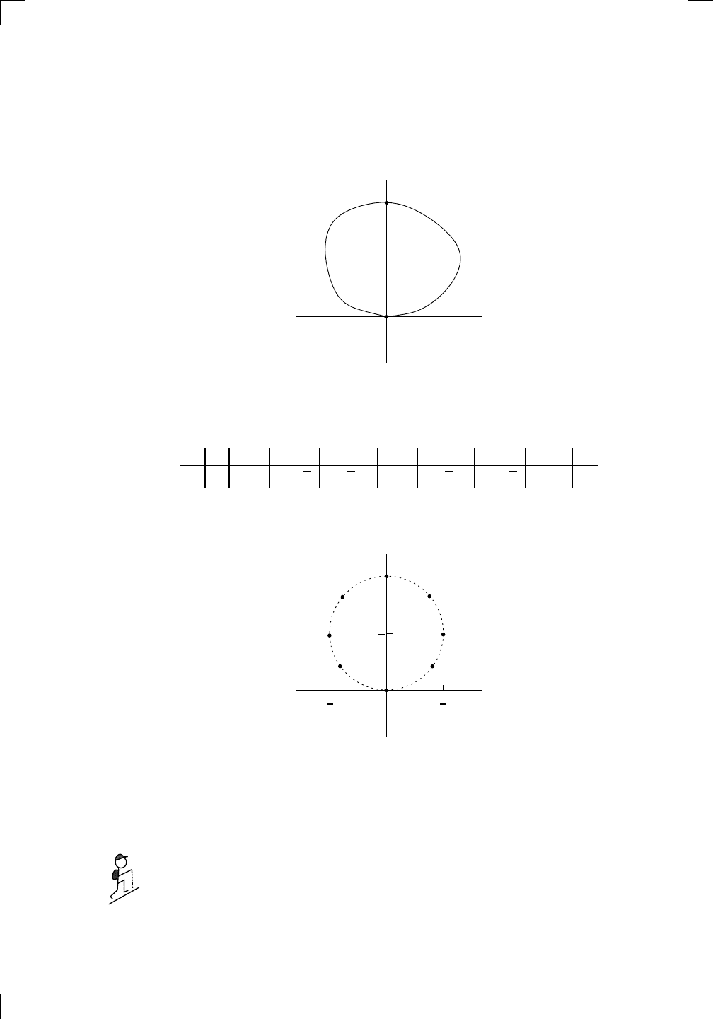
This shows that as the angle turns from 0 to π, the distance r increases from
0 up to 3, then heads back down to 0 by the time we get back to π. So the
curve we want looks something like this:
PSfrag
replacements
(
a, b)
[
a, b]
(
a, b]
[
a, b)
(
a, ∞)
[
a, ∞)
(
−∞, b)
(
−∞, b]
(
−∞, ∞)
{
x : a < x < b}
{
x : a ≤ x ≤ b}
{
x : a < x ≤ b}
{
x : a ≤ x < b}
{
x : x ≥ a}
{
x : x > a}
{
x : x ≤ b}
{
x : x < b}
R
a
b
shado
w
0
1
4
−
2
3
−
3
g(
x) = x
2
f(
x) = x
3
g(
x) = x
2
f(
x) = x
3
mirror
(y = x)
f
−
1
(x) =
3
√
x
y = h
(x)
y = h
−
1
(x)
y =
(x − 1)
2
−
1
x
Same
height
−
x
Same
length,
opp
osite signs
y = −
2x
−
2
1
y =
1
2
x − 1
2
−
1
y =
2
x
y =
10
x
y =
2
−x
y =
log
2
(x)
4
3
units
mirror
(x-axis)
y = |
x|
y = |
log
2
(x)|
θ radians
θ units
30
◦
=
π
6
45
◦
=
π
4
60
◦
=
π
3
120
◦
=
2
π
3
135
◦
=
3
π
4
150
◦
=
5
π
6
90
◦
=
π
2
180
◦
= π
210
◦
=
7
π
6
225
◦
=
5
π
4
240
◦
=
4
π
3
270
◦
=
3
π
2
300
◦
=
5
π
3
315
◦
=
7
π
4
330
◦
=
11
π
6
0
◦
=
0 radians
θ
hypotenuse
opp
osite
adjacen
t
0
(≡ 2π)
π
2
π
3
π
2
I
I
I
I
II
IV
θ
(
x, y)
x
y
r
7
π
6
reference
angle
reference
angle =
π
6
sin
+
sin −
cos
+
cos −
tan
+
tan −
A
S
T
C
7
π
4
9
π
13
5
π
6
(this
angle is
5π
6
clo
ckwise)
1
2
1
2
3
4
5
6
0
−
1
−
2
−
3
−
4
−
5
−
6
−
3π
−
5
π
2
−
2π
−
3
π
2
−
π
−
π
2
3
π
3
π
5
π
2
2
π
3
π
2
π
π
2
y =
sin(x)
1
0
−
1
−
3π
−
5
π
2
−
2π
−
3
π
2
−
π
−
π
2
3
π
5
π
2
2
π
2
π
3
π
2
π
π
2
y =
sin(x)
y =
cos(x)
−
π
2
π
2
y =
tan(x), −
π
2
<
x <
π
2
0
−
π
2
π
2
y =
tan(x)
−
2π
−
3π
−
5
π
2
−
3
π
2
−
π
−
π
2
π
2
3
π
3
π
5
π
2
2
π
3
π
2
π
y =
sec(x)
y =
csc(x)
y =
cot(x)
y = f (
x)
−
1
1
2
y = g(
x)
3
y = h
(x)
4
5
−
2
f(
x) =
1
x
g(
x) =
1
x
2
etc.
0
1
π
1
2
π
1
3
π
1
4
π
1
5
π
1
6
π
1
7
π
g(
x) = sin
1
x
1
0
−
1
L
10
100
200
y =
π
2
y = −
π
2
y =
tan
−1
(x)
π
2
π
y =
sin
(x)
x
,
x > 3
0
1
−
1
a
L
f(
x) = x sin (1/x)
(0 <
x < 0.3)
h
(x) = x
g(
x) = −x
a
L
lim
x
→a
+
f(x) = L
lim
x
→a
+
f(x) = ∞
lim
x
→a
+
f(x) = −∞
lim
x
→a
+
f(x) DNE
lim
x
→a
−
f(x) = L
lim
x
→a
−
f(x) = ∞
lim
x
→a
−
f(x) = −∞
lim
x
→a
−
f(x) DNE
M
}
lim
x
→a
−
f(x) = M
lim
x
→a
f(x) = L
lim
x
→a
f(x) DNE
lim
x
→∞
f(x) = L
lim
x
→∞
f(x) = ∞
lim
x
→∞
f(x) = −∞
lim
x
→∞
f(x) DNE
lim
x
→−∞
f(x) = L
lim
x
→−∞
f(x) = ∞
lim
x
→−∞
f(x) = −∞
lim
x
→−∞
f(x) DNE
lim
x →a
+
f(
x) = ∞
lim
x →a
+
f(
x) = −∞
lim
x →a
−
f(
x) = ∞
lim
x →a
−
f(
x) = −∞
lim
x →a
f(
x) = ∞
lim
x →a
f(
x) = −∞
lim
x →a
f(
x) DNE
y = f (
x)
a
y =
|
x|
x
1
−
1
y =
|
x + 2|
x +
2
1
−
1
−
2
1
2
3
4
a
a
b
y = x sin
1
x
y = x
y = −
x
a
b
c
d
C
a
b
c
d
−
1
0
1
2
3
time
y
t
u
(
t, f(t))
(
u, f(u))
time
y
t
u
y
x
(
x, f(x))
y = |
x|
(
z, f(z))
z
y = f (
x)
a
tangen
t at x = a
b
tangen
t at x = b
c
tangen
t at x = c
y = x
2
tangen
t
at x = −
1
u
v
uv
u +
∆u
v +
∆v
(
u + ∆u)(v + ∆v)
∆
u
∆
v
u
∆v
v∆
u
∆
u∆v
y = f (
x)
1
2
−
2
y = |
x
2
− 4|
y = x
2
− 4
y = −
2x + 5
y = g(
x)
1
2
3
4
5
6
7
8
9
0
−
1
−
2
−
3
−
4
−
5
−
6
y = f(
x)
3
−
3
3
−
3
0
−
1
2
easy
hard
flat
y = f
0
(
x)
3
−
3
0
−
1
2
1
−
1
y =
sin(x)
y = x
x
A
B
O
1
C
D
sin(
x)
tan(
x)
y =
sin
(x)
x
π
2
π
1
−
1
x =
0
a =
0
x
> 0
a
> 0
x
< 0
a
< 0
rest
position
+
−
y = x
2
sin
1
x
N
A
B
H
a
b
c
O
H
A
B
C
D
h
r
R
θ
1000
2000
α
β
p
h
y = g(
x) = log
b
(x)
y = f (
x) = b
x
y = e
x
5
10
1
2
3
4
0
−
1
−
2
−
3
−
4
y =
ln(x)
y =
cosh(x)
y =
sinh(x)
y =
tanh(x)
y =
sech(x)
y =
csch(x)
y =
coth(x)
1
−
1
y = f (
x)
original
function
in
verse function
slop
e = 0 at (x, y)
slop
e is infinite at (y, x)
−
108
2
5
1
2
1
2
3
4
5
6
0
−
1
−
2
−
3
−
4
−
5
−
6
−
3π
−
5
π
2
−
2π
−
3
π
2
−
π
−
π
2
3
π
3
π
5
π
2
2
π
3
π
2
π
π
2
y =
sin(x)
1
0
−
1
−
3π
−
5
π
2
−
2π
−
3
π
2
−
π
−
π
2
3
π
5
π
2
2
π
2
π
3
π
2
π
π
2
y =
sin(x)
y =
sin(x), −
π
2
≤ x ≤
π
2
−
2
−
1
0
2
π
2
−
π
2
y =
sin
−1
(x)
y =
cos(x)
π
π
2
y =
cos
−1
(x)
−
π
2
1
x
α
β
y =
tan(x)
y =
tan(x)
1
y =
tan
−1
(x)
y =
sec(x)
y =
sec
−1
(x)
y =
csc
−1
(x)
y =
cot
−1
(x)
1
y =
cosh
−1
(x)
y =
sinh
−1
(x)
y =
tanh
−1
(x)
y =
sech
−1
(x)
y =
csch
−1
(x)
y =
coth
−1
(x)
(0
, 3)
(2
, −1)
(5
, 2)
(7
, 0)
(
−1, 44)
(0
, 1)
(1
, −12)
(2
, 305)
y =
1
2
(2
, 3)
y = f (
x)
y = g(
x)
a
b
c
a
b
c
s
c
0
c
1
(
a, f(a))
(
b, f(b))
1
2
1
2
3
4
5
6
0
−
1
−
2
−
3
−
4
−
5
−
6
−
3π
−
5
π
2
−
2π
−
3
π
2
−
π
−
π
2
3
π
3
π
5
π
2
2
π
3
π
2
π
π
2
y =
sin(x)
1
0
−
1
−
3π
−
5
π
2
−
2π
−
3
π
2
−
π
−
π
2
3
π
5
π
2
2
π
2
π
3
π
2
π
π
2
c
OR
Lo
cal maximum
Lo
cal minimum
Horizon
tal point of inflection
1
e
y = f
0
(
x)
y = f(
x) = x ln(x)
−
1
e
?
y = f(
x) = x
3
y = g(
x) = x
4
x
f(
x)
−
3
−
2
−
1
0
1
2
1
2
3
4
+
−
?
1
5
6
3
f
0
(
x)
2 −
1
2
√
6
2
+
1
2
√
6
f
00
(
x)
7
8
g
00
(
x)
f
00
(
x)
0
y =
(
x − 3)(x − 1)
2
x
3
(
x + 2)
y = x ln
(x)
1
e
−
1
e
5
−
108
2
α
β
2 −
1
2
√
6
2
+
1
2
√
6
y = x
2
(
x − 5)
3
−
e
−
1/2
√
3
e
−
1/2
√
3
−
e
−3/2
e
−
3/2
−
1
√
3
1
√
3
−
1
1
y = xe
−
3x
2
/2
y =
x
3
− 6
x
2
+ 13x − 8
x
28
2
600
500
400
300
200
100
0
−
100
−
200
−
300
−
400
−
500
−
600
0
10
−
10
5
−
5
20
−
20
15
−
15
0
4
5
6
x
P
0
(
x)
+
−
−
existing
fence
new
fence
enclosure
A
h
b
H
99
100
101
h
dA/dh
r
h
1
2
7
shallo
w
deep
LAND
SEA
N
y
z
s
t
3
11
9
L
(11)
√
11
y = L
(x)
y = f(
x)
11
y = L
(x)
y = f (
x)
F
P
a
a +
∆x
f(
a + ∆x)
L
(a + ∆x)
f(
a)
error
d
f
∆
x
a
b
y = f (
x)
true
zero
starting
approximation
b
etter approximation
v
t
3
5
50
40
60
4
20
30
25
t
1
t
2
t
3
t
4
t
n
−2
t
n
−1
t
0
= a
t
n
= b
v
1
v
2
v
3
v
4
v
n
−1
v
n
−
30
6
30
|
v|
a
b
p
q
c
v(
c)
v(
c
1
)
v(
c
2
)
v(
c
3
)
v(
c
4
)
v(
c
5
)
v(
c
6
)
t
1
t
2
t
3
t
4
t
5
c
1
c
2
c
3
c
4
c
5
c
6
t
0
=
a
t
6
=
b
t
16
=
b
t
10
=
b
a
b
x
y
y = f (
x)
1
2
y = x
5
0
−
2
y =
1
a
b
y =
sin(x)
π
−
π
0
−
1
−
2
0
2
4
y = x
2
0
1
2
3
4
2
n
4
n
6
n
2(
n−2)
n
2(
n−1)
n
2
n
n
=
2
width
of each interval =
2
n
−
2
1
3
0
I
I
I
I
II
IV
4
y
dx
y = −
x
2
− 2x + 3
3
−
5
y = |−
x
2
− 2x + 3|
I
I
I
I
Ia
5
3
0
1
2
a
b
y = f (
x)
y = g(
x)
y = x
2
a
b
5
3
0
1
2
y =
√
x
2
√
2
2
2
dy
x
2
a
b
y = f (
x)
y = g(
x)
M
m
1
2
−
1
−
2
0
y = e
−
x
2
1
2
e
−
1/4
f
a
v
y = f
a
v
c
A
M
0
1
2
a
b
x
t
y = f(
t)
F (
x )
y = f(
t)
F (
x + h )
x + h
F (
x + h) − F (x)
f(
x)
1
2
y =
sin(x)
π
−
π
−
1
−
2
y =
1
x
y = x
2
1
2
1
−
1
y =
ln|x|
θ
a
x
a
x
p
a
2
− x
2
3
x
p
9 − x
2
p
x
2
+ a
2
x
a
p
x
2
+ 15
x
√
15
x
p
x
2
− a
2
a
x
p
x
2
− 4
2
x
−
p
x
2
− a
2
a
x
−
p
x
2
− 4
2
y = f (
x)
a
b
a + ε
ε
Z
b
a
+ε
f(x) dx
small
ev
en smaller
y = g(
x)
infinite
area
finite
area
1
y =
1
x
y =
1
x
p
, p < 1 (typical)
y =
1
x
p
, p > 1 (typical)
a
1
a
2
a
3
a
4
a
5
a
6
a
7
a
8
1
2
3
4
5
6
7
8
n
a
n
x
y
y = f (x)
(a, f(a))
a
−1
0
1
a
6
1
2
7
1
2
7
?
−2
−1
−2
t = 0
t = π/6
t = π/4
t = π/3
t = π/2
3
0
t = −2
t = −3/2
t = ±1
t = −1/2
t = 0
t = 1/2
t = 3/2
t = 2
12
−12
θ
r
P
θ
r
P
11π
6
2
(−1, −1)
wrong point
π
4
5π
4
√
2
(0, 1)
(0, −3)
(−2, 0)
π
2
3π
2
π
r = 3 sin(θ)
3π
2
θ
2π
1
0
−1
−2
−3
0
This looks a little pathetic. To tighten it up, we can write down the following
table of values:
θ 0 π/6 π/4 π/3 π/2 2π/3 3π/4 5π/6 π
r 0 3/2 3/
√
2 3
√
3/2 3 3
√
3/2 3/
√
2 3/2 0
Plotting these points leads to the following picture:
PSfrag
replacements
(
a, b)
[
a, b]
(
a, b]
[
a, b)
(
a, ∞)
[
a, ∞)
(
−∞, b)
(
−∞, b]
(
−∞, ∞)
{
x : a < x < b}
{
x : a ≤ x ≤ b}
{
x : a < x ≤ b}
{
x : a ≤ x < b}
{
x : x ≥ a}
{
x : x > a}
{
x : x ≤ b}
{
x : x < b}
R
a
b
shado
w
0
1
4
−
2
3
−
3
g(
x) = x
2
f(
x) = x
3
g(
x) = x
2
f(
x) = x
3
mirror
(y = x)
f
−
1
(x) =
3
√
x
y = h
(x)
y = h
−
1
(x)
y =
(x − 1)
2
−
1
x
Same
height
−
x
Same
length,
opp
osite signs
y = −
2x
−
2
1
y =
1
2
x − 1
2
−
1
y =
2
x
y =
10
x
y =
2
−x
y =
log
2
(x)
4
3
units
mirror
(x-axis)
y = |
x|
y = |
log
2
(x)|
θ radians
θ units
30
◦
=
π
6
45
◦
=
π
4
60
◦
=
π
3
120
◦
=
2
π
3
135
◦
=
3
π
4
150
◦
=
5
π
6
90
◦
=
π
2
180
◦
= π
210
◦
=
7
π
6
225
◦
=
5
π
4
240
◦
=
4
π
3
270
◦
=
3
π
2
300
◦
=
5
π
3
315
◦
=
7
π
4
330
◦
=
11
π
6
0
◦
=
0 radians
θ
hypotenuse
opp
osite
adjacen
t
0
(≡ 2π)
π
2
π
3
π
2
I
I
I
I
II
IV
θ
(
x, y)
x
y
r
7
π
6
reference
angle
reference
angle =
π
6
sin
+
sin −
cos
+
cos −
tan
+
tan −
A
S
T
C
7
π
4
9
π
13
5
π
6
(this
angle is
5π
6
clo
ckwise)
1
2
1
2
3
4
5
6
0
−
1
−
2
−
3
−
4
−
5
−
6
−
3π
−
5
π
2
−
2π
−
3
π
2
−
π
−
π
2
3
π
3
π
5
π
2
2
π
3
π
2
π
π
2
y =
sin(x)
1
0
−
1
−
3π
−
5
π
2
−
2π
−
3
π
2
−
π
−
π
2
3
π
5
π
2
2
π
2
π
3
π
2
π
π
2
y =
sin(x)
y =
cos(x)
−
π
2
π
2
y =
tan(x), −
π
2
<
x <
π
2
0
−
π
2
π
2
y =
tan(x)
−
2π
−
3π
−
5
π
2
−
3
π
2
−
π
−
π
2
π
2
3
π
3
π
5
π
2
2
π
3
π
2
π
y =
sec(x)
y =
csc(x)
y =
cot(x)
y = f (
x)
−
1
1
2
y = g(
x)
3
y = h
(x)
4
5
−
2
f(
x) =
1
x
g(
x) =
1
x
2
etc.
0
1
π
1
2
π
1
3
π
1
4
π
1
5
π
1
6
π
1
7
π
g(
x) = sin
1
x
1
0
−
1
L
10
100
200
y =
π
2
y = −
π
2
y =
tan
−1
(x)
π
2
π
y =
sin
(x)
x
,
x > 3
0
1
−
1
a
L
f(
x) = x sin (1/x)
(0 <
x < 0.3)
h
(x) = x
g(
x) = −x
a
L
lim
x
→a
+
f(x) = L
lim
x
→a
+
f(x) = ∞
lim
x
→a
+
f(x) = −∞
lim
x
→a
+
f(x) DNE
lim
x
→a
−
f(x) = L
lim
x
→a
−
f(x) = ∞
lim
x
→a
−
f(x) = −∞
lim
x
→a
−
f(x) DNE
M
}
lim
x
→a
−
f(x) = M
lim
x
→a
f(x) = L
lim
x
→a
f(x) DNE
lim
x
→∞
f(x) = L
lim
x
→∞
f(x) = ∞
lim
x
→∞
f(x) = −∞
lim
x
→∞
f(x) DNE
lim
x
→−∞
f(x) = L
lim
x
→−∞
f(x) = ∞
lim
x
→−∞
f(x) = −∞
lim
x
→−∞
f(x) DNE
lim
x →a
+
f(
x) = ∞
lim
x →a
+
f(
x) = −∞
lim
x →a
−
f(
x) = ∞
lim
x →a
−
f(
x) = −∞
lim
x →a
f(
x) = ∞
lim
x →a
f(
x) = −∞
lim
x →a
f(
x) DNE
y = f (
x)
a
y =
|
x|
x
1
−
1
y =
|
x + 2|
x +
2
1
−
1
−
2
1
2
3
4
a
a
b
y = x sin
1
x
y = x
y = −
x
a
b
c
d
C
a
b
c
d
−
1
0
1
2
3
time
y
t
u
(
t, f(t))
(
u, f(u))
time
y
t
u
y
x
(
x, f(x))
y = |
x|
(
z, f(z))
z
y = f (
x)
a
tangen
t at x = a
b
tangen
t at x = b
c
tangen
t at x = c
y = x
2
tangen
t
at x = −
1
u
v
uv
u +
∆u
v +
∆v
(
u + ∆u)(v + ∆v)
∆
u
∆
v
u
∆v
v∆
u
∆
u∆v
y = f (
x)
1
2
−
2
y = |
x
2
− 4|
y = x
2
− 4
y = −
2x + 5
y = g(
x)
1
2
3
4
5
6
7
8
9
0
−
1
−
2
−
3
−
4
−
5
−
6
y = f(
x)
3
−
3
3
−
3
0
−
1
2
easy
hard
flat
y = f
0
(
x)
3
−
3
0
−
1
2
1
−
1
y =
sin(x)
y = x
x
A
B
O
1
C
D
sin(
x)
tan(
x)
y =
sin
(x)
x
π
2
π
1
−
1
x =
0
a =
0
x
> 0
a
> 0
x
< 0
a
< 0
rest
position
+
−
y = x
2
sin
1
x
N
A
B
H
a
b
c
O
H
A
B
C
D
h
r
R
θ
1000
2000
α
β
p
h
y = g(
x) = log
b
(x)
y = f (
x) = b
x
y = e
x
5
10
1
2
3
4
0
−
1
−
2
−
3
−
4
y =
ln(x)
y =
cosh(x)
y =
sinh(x)
y =
tanh(x)
y =
sech(x)
y =
csch(x)
y =
coth(x)
1
−
1
y = f (
x)
original
function
in
verse function
slop
e = 0 at (x, y)
slop
e is infinite at (y, x)
−
108
2
5
1
2
1
2
3
4
5
6
0
−
1
−
2
−
3
−
4
−
5
−
6
−
3π
−
5
π
2
−
2π
−
3
π
2
−
π
−
π
2
3
π
3
π
5
π
2
2
π
3
π
2
π
π
2
y =
sin(x)
1
0
−
1
−
3π
−
5
π
2
−
2π
−
3
π
2
−
π
−
π
2
3
π
5
π
2
2
π
2
π
3
π
2
π
π
2
y =
sin(x)
y =
sin(x), −
π
2
≤ x ≤
π
2
−
2
−
1
0
2
π
2
−
π
2
y =
sin
−1
(x)
y =
cos(x)
π
π
2
y =
cos
−1
(x)
−
π
2
1
x
α
β
y =
tan(x)
y =
tan(x)
1
y =
tan
−1
(x)
y =
sec(x)
y =
sec
−1
(x)
y =
csc
−1
(x)
y =
cot
−1
(x)
1
y =
cosh
−1
(x)
y =
sinh
−1
(x)
y =
tanh
−1
(x)
y =
sech
−1
(x)
y =
csch
−1
(x)
y =
coth
−1
(x)
(0
, 3)
(2
, −1)
(5
, 2)
(7
, 0)
(
−1, 44)
(0
, 1)
(1
, −12)
(2
, 305)
y =
1
2
(2
, 3)
y = f (
x)
y = g(
x)
a
b
c
a
b
c
s
c
0
c
1
(
a, f(a))
(
b, f(b))
1
2
1
2
3
4
5
6
0
−
1
−
2
−
3
−
4
−
5
−
6
−
3π
−
5
π
2
−
2π
−
3
π
2
−
π
−
π
2
3
π
3
π
5
π
2
2
π
3
π
2
π
π
2
y =
sin(x)
1
0
−
1
−
3π
−
5
π
2
−
2π
−
3
π
2
−
π
−
π
2
3
π
5
π
2
2
π
2
π
3
π
2
π
π
2
c
OR
Lo
cal maximum
Lo
cal minimum
Horizon
tal point of inflection
1
e
y = f
0
(
x)
y = f(
x) = x ln(x)
−
1
e
?
y = f(
x) = x
3
y = g(
x) = x
4
x
f(
x)
−
3
−
2
−
1
0
1
2
1
2
3
4
+
−
?
1
5
6
3
f
0
(
x)
2 −
1
2
√
6
2
+
1
2
√
6
f
00
(
x)
7
8
g
00
(
x)
f
00
(
x)
0
y =
(
x − 3)(x − 1)
2
x
3
(
x + 2)
y = x ln
(x)
1
e
−
1
e
5
−
108
2
α
β
2 −
1
2
√
6
2
+
1
2
√
6
y = x
2
(
x − 5)
3
−
e
−
1/2
√
3
e
−
1/2
√
3
−
e
−3/2
e
−
3/2
−
1
√
3
1
√
3
−
1
1
y = xe
−
3x
2
/2
y =
x
3
− 6
x
2
+ 13x − 8
x
28
2
600
500
400
300
200
100
0
−
100
−
200
−
300
−
400
−
500
−
600
0
10
−
10
5
−
5
20
−
20
15
−
15
0
4
5
6
x
P
0
(
x)
+
−
−
existing
fence
new
fence
enclosure
A
h
b
H
99
100
101
h
dA/dh
r
h
1
2
7
shallo
w
deep
LAND
SEA
N
y
z
s
t
3
11
9
L
(11)
√
11
y = L
(x)
y = f(
x)
11
y = L
(x)
y = f (
x)
F
P
a
a +
∆x
f(
a + ∆x)
L
(a + ∆x)
f(
a)
error
d
f
∆
x
a
b
y = f (
x)
true
zero
starting
approximation
b
etter approximation
v
t
3
5
50
40
60
4
20
30
25
t
1
t
2
t
3
t
4
t
n
−2
t
n
−1
t
0
= a
t
n
= b
v
1
v
2
v
3
v
4
v
n
−1
v
n
−
30
6
30
|
v|
a
b
p
q
c
v(
c)
v(
c
1
)
v(
c
2
)
v(
c
3
)
v(
c
4
)
v(
c
5
)
v(
c
6
)
t
1
t
2
t
3
t
4
t
5
c
1
c
2
c
3
c
4
c
5
c
6
t
0
=
a
t
6
=
b
t
16
=
b
t
10
=
b
a
b
x
y
y = f (
x)
1
2
y = x
5
0
−
2
y =
1
a
b
y =
sin(x)
π
−
π
0
−
1
−
2
0
2
4
y = x
2
0
1
2
3
4
2
n
4
n
6
n
2(
n−2)
n
2(
n−1)
n
2
n
n
=
2
width
of each interval =
2
n
−
2
1
3
0
I
I
I
I
II
IV
4
y
dx
y = −
x
2
− 2x + 3
3
−
5
y = |−
x
2
− 2x + 3|
I
I
I
I
Ia
5
3
0
1
2
a
b
y = f (
x)
y = g(
x)
y = x
2
a
b
5
3
0
1
2
y =
√
x
2
√
2
2
2
dy
x
2
a
b
y = f (
x)
y = g(
x)
M
m
1
2
−
1
−
2
0
y = e
−
x
2
1
2
e
−
1/4
f
a
v
y = f
a
v
c
A
M
0
1
2
a
b
x
t
y = f(
t)
F (
x )
y = f(
t)
F (
x + h )
x + h
F (
x + h) − F (x)
f(
x)
1
2
y =
sin(x)
π
−
π
−
1
−
2
y =
1
x
y = x
2
1
2
1
−
1
y =
ln|x|
θ
a
x
a
x
p
a
2
− x
2
3
x
p
9 − x
2
p
x
2
+ a
2
x
a
p
x
2
+ 15
x
√
15
x
p
x
2
− a
2
a
x
p
x
2
− 4
2
x
−
p
x
2
− a
2
a
x
−
p
x
2
− 4
2
y = f (x)
a
b
a + ε
ε
Z
b
a+ε
f(x) dx
small
even smaller
y = g(x)
infinite area
finite area
1
y =
1
x
y =
1
x
p
, p < 1 (typical)
y =
1
x
p
, p > 1 (typical)
a
1
a
2
a
3
a
4
a
5
a
6
a
7
a
8
1
2
3
4
5
6
7
8
n
a
n
x
y
y = f (x)
(a, f(a))
a
−1
0
1
a
6
1
2
7
1
2
7
?
−2
−1
−2
t = 0
t = π/6
t = π/4
t = π/3
t = π/2
3
0
t = −2
t = −3/2
t = ±1
t = −1/2
t = 0
t = 1/2
t = 3/2
t = 2
12
−12
θ
r
P
θ
r
P
11π
6
2
(−1, −1)
wrong point
π
4
5π
4
√
2
(0, 1)
(0, −3)
(−2, 0)
π
2
3π
2
π
r = 3 sin(θ)
3π
2
θ
2π
1
0
−1
−2
−3
0
3
2
3
2
−
3
2
0
So it actually looks like a real circle, not a pathetic one like our first attempt.
In fact, we can check that it is a circle by converting to Cartesian coordinates.
Indeed, since y = r sin(θ), and we have r = 3 sin(θ), we can eliminate θ and
get r
2
= 3y. On the other hand, r
2
= x
2
+ y
2
, so we get x
2
+ y
2
= 3y.
Putting the 3y on the left-hand side and completing the square in y, we get
x
2
+(y−3/2)
2
= (3/2)
2
, which is the equation of the circle with center (0, 3/2)
and radius 3/2 units. This agrees with the above picture. Now, you should
PSfrag
replacements
(
a, b)
[
a, b]
(
a, b]
[
a, b)
(
a, ∞)
[
a, ∞)
(
−∞, b)
(
−∞, b]
(
−∞, ∞)
{
x : a < x < b}
{
x : a ≤ x ≤ b}
{
x : a < x ≤ b}
{
x : a ≤ x < b}
{
x : x ≥ a}
{
x : x > a}
{
x : x ≤ b}
{
x : x < b}
R
a
b
shado
w
0
1
4
−
2
3
−
3
g(
x) = x
2
f(
x) = x
3
g(
x) = x
2
f(
x) = x
3
mirror
(y = x)
f
−
1
(x) =
3
√
x
y = h
(x)
y = h
−
1
(x)
y =
(x − 1)
2
−
1
x
Same
height
−
x
Same
length,
opp
osite signs
y = −
2x
−
2
1
y =
1
2
x − 1
2
−
1
y =
2
x
y =
10
x
y =
2
−x
y =
log
2
(x)
4
3
units
mirror
(x-axis)
y = |
x|
y = |
log
2
(x)|
θ radians
θ units
30
◦
=
π
6
45
◦
=
π
4
60
◦
=
π
3
120
◦
=
2
π
3
135
◦
=
3
π
4
150
◦
=
5
π
6
90
◦
=
π
2
180
◦
= π
210
◦
=
7
π
6
225
◦
=
5
π
4
240
◦
=
4
π
3
270
◦
=
3
π
2
300
◦
=
5
π
3
315
◦
=
7
π
4
330
◦
=
11
π
6
0
◦
=
0 radians
θ
hypotenuse
opp
osite
adjacen
t
0
(≡ 2π)
π
2
π
3
π
2
I
I
I
I
II
IV
θ
(
x, y)
x
y
r
7
π
6
reference
angle
reference
angle =
π
6
sin
+
sin −
cos
+
cos −
tan
+
tan −
A
S
T
C
7
π
4
9
π
13
5
π
6
(this
angle is
5π
6
clo
ckwise)
1
2
1
2
3
4
5
6
0
−
1
−
2
−
3
−
4
−
5
−
6
−
3π
−
5
π
2
−
2π
−
3
π
2
−
π
−
π
2
3
π
3
π
5
π
2
2
π
3
π
2
π
π
2
y =
sin(x)
1
0
−
1
−
3π
−
5
π
2
−
2π
−
3
π
2
−
π
−
π
2
3
π
5
π
2
2
π
2
π
3
π
2
π
π
2
y =
sin(x)
y =
cos(x)
−
π
2
π
2
y =
tan(x), −
π
2
<
x <
π
2
0
−
π
2
π
2
y =
tan(x)
−
2π
−
3π
−
5
π
2
−
3
π
2
−
π
−
π
2
π
2
3
π
3
π
5
π
2
2
π
3
π
2
π
y =
sec(x)
y =
csc(x)
y =
cot(x)
y = f(
x)
−
1
1
2
y = g(
x)
3
y = h
(x)
4
5
−
2
f(
x) =
1
x
g(
x) =
1
x
2
etc.
0
1
π
1
2
π
1
3
π
1
4
π
1
5
π
1
6
π
1
7
π
g(
x) = sin
1
x
1
0
−
1
L
10
100
200
y =
π
2
y = −
π
2
y =
tan
−1
(x)
π
2
π
y =
sin(
x)
x
,
x > 3
0
1
−
1
a
L
f(
x) = x sin (1/x)
(0 <
x < 0.3)
h
(x) = x
g(
x) = −x
a
L
lim
x
→a
+
f(x) = L
lim
x
→a
+
f(x) = ∞
lim
x
→a
+
f(x) = −∞
lim
x
→a
+
f(x) DNE
lim
x
→a
−
f(x) = L
lim
x
→a
−
f(x) = ∞
lim
x
→a
−
f(x) = −∞
lim
x
→a
−
f(x) DNE
M
}
lim
x
→a
−
f(x) = M
lim
x
→a
f(x) = L
lim
x
→a
f(x) DNE
lim
x
→∞
f(x) = L
lim
x
→∞
f(x) = ∞
lim
x
→∞
f(x) = −∞
lim
x
→∞
f(x) DNE
lim
x
→−∞
f(x) = L
lim
x
→−∞
f(x) = ∞
lim
x
→−∞
f(x) = −∞
lim
x
→−∞
f(x) DNE
lim
x →a
+
f(
x) = ∞
lim
x →a
+
f(
x) = −∞
lim
x →a
−
f(
x) = ∞
lim
x →a
−
f(
x) = −∞
lim
x →a
f(
x) = ∞
lim
x →a
f(
x) = −∞
lim
x →a
f(
x) DNE
y = f (
x)
a
y =
|
x|
x
1
−
1
y =
|
x + 2|
x +
2
1
−
1
−
2
1
2
3
4
a
a
b
y = x sin
1
x
y = x
y = −
x
a
b
c
d
C
a
b
c
d
−
1
0
1
2
3
time
y
t
u
(
t, f(t))
(
u, f(u))
time
y
t
u
y
x
(
x, f(x))
y = |
x|
(
z, f(z))
z
y = f(
x)
a
tangen
t at x = a
b
tangen
t at x = b
c
tangen
t at x = c
y = x
2
tangen
t
at x = −
1
u
v
uv
u +
∆u
v +
∆v
(
u + ∆u)(v + ∆v)
∆
u
∆
v
u
∆v
v∆
u
∆
u∆v
y = f(
x)
1
2
−
2
y = |
x
2
− 4|
y = x
2
− 4
y = −
2x + 5
y = g(
x)
1
2
3
4
5
6
7
8
9
0
−
1
−
2
−
3
−
4
−
5
−
6
y = f (
x)
3
−
3
3
−
3
0
−
1
2
easy
hard
flat
y = f
0
(
x)
3
−
3
0
−
1
2
1
−
1
y =
sin(x)
y = x
x
A
B
O
1
C
D
sin(
x)
tan(
x)
y =
sin(
x)
x
π
2
π
1
−
1
x =
0
a =
0
x
> 0
a
> 0
x
< 0
a
< 0
rest
position
+
−
y = x
2
sin
1
x
N
A
B
H
a
b
c
O
H
A
B
C
D
h
r
R
θ
1000
2000
α
β
p
h
y = g(
x) = log
b
(x)
y = f(
x) = b
x
y = e
x
5
10
1
2
3
4
0
−
1
−
2
−
3
−
4
y =
ln(x)
y =
cosh(x)
y =
sinh(x)
y =
tanh(x)
y =
sech(x)
y =
csch(x)
y =
coth(x)
1
−
1
y = f(
x)
original
function
in
verse function
slop
e = 0 at (x, y)
slop
e is infinite at (y, x)
−
108
2
5
1
2
1
2
3
4
5
6
0
−
1
−
2
−
3
−
4
−
5
−
6
−
3π
−
5
π
2
−
2π
−
3
π
2
−
π
−
π
2
3
π
3
π
5
π
2
2
π
3
π
2
π
π
2
y =
sin(x)
1
0
−
1
−
3π
−
5
π
2
−
2π
−
3
π
2
−
π
−
π
2
3
π
5
π
2
2
π
2
π
3
π
2
π
π
2
y =
sin(x)
y =
sin(x), −
π
2
≤ x ≤
π
2
−
2
−
1
0
2
π
2
−
π
2
y =
sin
−1
(x)
y =
cos(x)
π
π
2
y =
cos
−1
(x)
−
π
2
1
x
α
β
y =
tan(x)
y =
tan(x)
1
y =
tan
−1
(x)
y =
sec(x)
y =
sec
−1
(x)
y =
csc
−1
(x)
y =
cot
−1
(x)
1
y =
cosh
−1
(x)
y =
sinh
−1
(x)
y =
tanh
−1
(x)
y =
sech
−1
(x)
y =
csch
−1
(x)
y =
coth
−1
(x)
(0
, 3)
(2
, −1)
(5
, 2)
(7
, 0)
(
−1, 44)
(0
, 1)
(1
, −12)
(2
, 305)
y =
1
2
(2
, 3)
y = f(
x)
y = g(
x)
a
b
c
a
b
c
s
c
0
c
1
(
a, f(a))
(
b, f(b))
1
2
1
2
3
4
5
6
0
−
1
−
2
−
3
−
4
−
5
−
6
−
3π
−
5
π
2
−
2π
−
3
π
2
−
π
−
π
2
3
π
3
π
5
π
2
2
π
3
π
2
π
π
2
y =
sin(x)
1
0
−
1
−
3π
−
5
π
2
−
2π
−
3
π
2
−
π
−
π
2
3
π
5
π
2
2
π
2
π
3
π
2
π
π
2
c
OR
Lo
cal maximum
Lo
cal minimum
Horizon
tal point of inflection
1
e
y = f
0
(
x)
y = f (
x) = x ln(x)
−
1
e
?
y = f(
x) = x
3
y = g(
x) = x
4
x
f(
x)
−
3
−
2
−
1
0
1
2
1
2
3
4
+
−
?
1
5
6
3
f
0
(
x)
2 −
1
2
√
6
2
+
1
2
√
6
f
00
(
x)
7
8
g
00
(
x)
f
00
(
x)
0
y =
(
x − 3)(x − 1)
2
x
3
(
x + 2)
y = x ln
(x)
1
e
−
1
e
5
−
108
2
α
β
2 −
1
2
√
6
2
+
1
2
√
6
y = x
2
(
x − 5)
3
−
e
−
1/2
√
3
e
−
1/2
√
3
−
e
−3/2
e
−
3/2
−
1
√
3
1
√
3
−
1
1
y = xe
−
3x
2
/2
y =
x
3
− 6
x
2
+ 13x − 8
x
28
2
600
500
400
300
200
100
0
−
100
−
200
−
300
−
400
−
500
−
600
0
10
−
10
5
−
5
20
−
20
15
−
15
0
4
5
6
x
P
0
(
x)
+
−
−
existing
fence
new
fence
enclosure
A
h
b
H
99
100
101
h
dA/dh
r
h
1
2
7
shallo
w
deep
LAND
SEA
N
y
z
s
t
3
11
9
L
(11)
√
11
y = L
(x)
y = f (
x)
11
y = L
(x)
y = f(
x)
F
P
a
a +
∆x
f(
a + ∆x)
L
(a + ∆x)
f(
a)
error
d
f
∆
x
a
b
y = f(
x)
true
zero
starting
approximation
b
etter approximation
v
t
3
5
50
40
60
4
20
30
25
t
1
t
2
t
3
t
4
t
n
−2
t
n
−1
t
0
= a
t
n
= b
v
1
v
2
v
3
v
4
v
n
−1
v
n
−
30
6
30
|
v|
a
b
p
q
c
v(
c)
v(
c
1
)
v(
c
2
)
v(
c
3
)
v(
c
4
)
v(
c
5
)
v(
c
6
)
t
1
t
2
t
3
t
4
t
5
c
1
c
2
c
3
c
4
c
5
c
6
t
0
=
a
t
6
=
b
t
16
=
b
t
10
=
b
a
b
x
y
y = f(
x)
1
2
y = x
5
0
−
2
y =
1
a
b
y =
sin(x)
π
−
π
0
−
1
−
2
0
2
4
y = x
2
0
1
2
3
4
2
n
4
n
6
n
2(
n−2)
n
2(
n−1)
n
2
n
n
=
2
width
of each interval =
2
n
−
2
1
3
0
I
I
I
I
II
IV
4
y
dx
y = −
x
2
− 2x + 3
3
−
5
y = |−
x
2
− 2x + 3|
I
I
I
I
Ia
5
3
0
1
2
a
b
y = f (
x)
y = g(
x)
y = x
2
a
b
5
3
0
1
2
y =
√
x
2
√
2
2
2
dy
x
2
a
b
y = f(
x)
y = g(
x)
M
m
1
2
−
1
−
2
0
y = e
−
x
2
1
2
e
−
1/4
f
a
v
y = f
a
v
c
A
M
0
1
2
a
b
x
t
y = f (
t)
F (
x )
y = f (
t)
F (
x + h)
x + h
F (
x + h) − F (x)
f(
x)
1
2
y =
sin(x)
π
−
π
−
1
−
2
y =
1
x
y = x
2
1
2
1
−
1
y =
ln|x|
θ
a
x
a
x
p
a
2
− x
2
3
x
p
9 − x
2
p
x
2
+ a
2
x
a
p
x
2
+ 15
x
√
15
x
p
x
2
− a
2
a
x
p
x
2
− 4
2
x
−
p
x
2
− a
2
a
x
−
p
x
2
− 4
2
y = f(x)
a
b
a + ε
ε
Z
b
a+ε
f(x) dx
small
even smaller
y = g(x)
infinite area
finite area
1
y =
1
x
y =
1
x
p
, p < 1 (typical)
y =
1
x
p
, p > 1 (typical)
a
1
a
2
a
3
a
4
a
5
a
6
a
7
a
8
1
2
3
4
5
6
7
8
n
a
n
x
y
y = f(x)
(a, f(a))
a
−1
0
1
a
6
1
2
7
1
2
7
?
−2
−1
−2
t = 0
t = π/6
t = π/4
t = π/3
t = π/2
3
0
t = −2
t = −3/2
t = ±1
t = −1/2
t = 0
t = 1/2
t = 3/2
t = 2
12
−12
θ
r
P
θ
r
P
11π
6
2
(−1, −1)
wrong point
π
4
5π
4
√
2
(0, 1)
(0, −3)
(−2, 0)
π
2
3π
2
π
r = 3 sin(θ)
3π
2
θ
2π
1
0
−1
−2
−3
0
3
2
−
3
2
0
try to convince yourself that if θ goes from π to 2π, you just end up retracing
the same circle again.
Section 27.2.2: Sketching curves in polar coordinates • 587
Let’s look at another example. Suppose that we want to sketch the curve
PSfrag
replacements
(
a, b)
[
a, b]
(
a, b]
[
a, b)
(
a, ∞)
[
a, ∞)
(
−∞, b)
(
−∞, b]
(
−∞, ∞)
{
x : a < x < b}
{
x : a ≤ x ≤ b}
{
x : a < x ≤ b}
{
x : a ≤ x < b}
{
x : x ≥ a}
{
x : x > a}
{
x : x ≤ b}
{
x : x < b}
R
a
b
shado
w
0
1
4
−
2
3
−
3
g(
x) = x
2
f(
x) = x
3
g(
x) = x
2
f(
x) = x
3
mirror
(y = x)
f
−
1
(x) =
3
√
x
y = h
(x)
y = h
−
1
(x)
y =
(x − 1)
2
−
1
x
Same
height
−
x
Same
length,
opp
osite signs
y = −
2x
−
2
1
y =
1
2
x − 1
2
−
1
y =
2
x
y =
10
x
y =
2
−x
y =
log
2
(x)
4
3
units
mirror
(x-axis)
y = |
x|
y = |
log
2
(x)|
θ radians
θ units
30
◦
=
π
6
45
◦
=
π
4
60
◦
=
π
3
120
◦
=
2
π
3
135
◦
=
3
π
4
150
◦
=
5
π
6
90
◦
=
π
2
180
◦
= π
210
◦
=
7
π
6
225
◦
=
5
π
4
240
◦
=
4
π
3
270
◦
=
3
π
2
300
◦
=
5
π
3
315
◦
=
7
π
4
330
◦
=
11
π
6
0
◦
=
0 radians
θ
hypotenuse
opp
osite
adjacen
t
0
(≡ 2π)
π
2
π
3
π
2
I
I
I
I
II
IV
θ
(
x, y)
x
y
r
7
π
6
reference
angle
reference
angle =
π
6
sin
+
sin −
cos
+
cos −
tan
+
tan −
A
S
T
C
7
π
4
9
π
13
5
π
6
(this
angle is
5π
6
clo
ckwise)
1
2
1
2
3
4
5
6
0
−
1
−
2
−
3
−
4
−
5
−
6
−
3π
−
5
π
2
−
2π
−
3
π
2
−
π
−
π
2
3
π
3
π
5
π
2
2
π
3
π
2
π
π
2
y =
sin(x)
1
0
−
1
−
3π
−
5
π
2
−
2π
−
3
π
2
−
π
−
π
2
3
π
5
π
2
2
π
2
π
3
π
2
π
π
2
y =
sin(x)
y =
cos(x)
−
π
2
π
2
y =
tan(x), −
π
2
<
x <
π
2
0
−
π
2
π
2
y =
tan(x)
−
2π
−
3π
−
5
π
2
−
3
π
2
−
π
−
π
2
π
2
3
π
3
π
5
π
2
2
π
3
π
2
π
y =
sec(x)
y =
csc(x)
y =
cot(x)
y = f(
x)
−
1
1
2
y = g(
x)
3
y = h
(x)
4
5
−
2
f(
x) =
1
x
g(
x) =
1
x
2
etc.
0
1
π
1
2
π
1
3
π
1
4
π
1
5
π
1
6
π
1
7
π
g(
x) = sin
1
x
1
0
−
1
L
10
100
200
y =
π
2
y = −
π
2
y =
tan
−1
(x)
π
2
π
y =
sin(
x)
x
,
x > 3
0
1
−
1
a
L
f(
x) = x sin (1/x)
(0 <
x < 0.3)
h
(x) = x
g(
x) = −x
a
L
lim
x
→a
+
f(x) = L
lim
x
→a
+
f(x) = ∞
lim
x
→a
+
f(x) = −∞
lim
x
→a
+
f(x) DNE
lim
x
→a
−
f(x) = L
lim
x
→a
−
f(x) = ∞
lim
x
→a
−
f(x) = −∞
lim
x
→a
−
f(x) DNE
M
}
lim
x
→a
−
f(x) = M
lim
x
→a
f(x) = L
lim
x
→a
f(x) DNE
lim
x
→∞
f(x) = L
lim
x
→∞
f(x) = ∞
lim
x
→∞
f(x) = −∞
lim
x
→∞
f(x) DNE
lim
x
→−∞
f(x) = L
lim
x
→−∞
f(x) = ∞
lim
x
→−∞
f(x) = −∞
lim
x
→−∞
f(x) DNE
lim
x →a
+
f(
x) = ∞
lim
x →a
+
f(
x) = −∞
lim
x →a
−
f(
x) = ∞
lim
x →a
−
f(
x) = −∞
lim
x →a
f(
x) = ∞
lim
x →a
f(
x) = −∞
lim
x →a
f(
x) DNE
y = f (
x)
a
y =
|
x|
x
1
−
1
y =
|
x + 2|
x +
2
1
−
1
−
2
1
2
3
4
a
a
b
y = x sin
1
x
y = x
y = −
x
a
b
c
d
C
a
b
c
d
−
1
0
1
2
3
time
y
t
u
(
t, f(t))
(
u, f(u))
time
y
t
u
y
x
(
x, f(x))
y = |
x|
(
z, f(z))
z
y = f(
x)
a
tangen
t at x = a
b
tangen
t at x = b
c
tangen
t at x = c
y = x
2
tangen
t
at x = −
1
u
v
uv
u +
∆u
v +
∆v
(
u + ∆u)(v + ∆v)
∆
u
∆
v
u
∆v
v∆
u
∆
u∆v
y = f(
x)
1
2
−
2
y = |
x
2
− 4|
y = x
2
− 4
y = −
2x + 5
y = g(
x)
1
2
3
4
5
6
7
8
9
0
−
1
−
2
−
3
−
4
−
5
−
6
y = f (
x)
3
−
3
3
−
3
0
−
1
2
easy
hard
flat
y = f
0
(
x)
3
−
3
0
−
1
2
1
−
1
y =
sin(x)
y = x
x
A
B
O
1
C
D
sin(
x)
tan(
x)
y =
sin(
x)
x
π
2
π
1
−
1
x =
0
a =
0
x
> 0
a
> 0
x
< 0
a
< 0
rest
position
+
−
y = x
2
sin
1
x
N
A
B
H
a
b
c
O
H
A
B
C
D
h
r
R
θ
1000
2000
α
β
p
h
y = g(
x) = log
b
(x)
y = f(
x) = b
x
y = e
x
5
10
1
2
3
4
0
−
1
−
2
−
3
−
4
y =
ln(x)
y =
cosh(x)
y =
sinh(x)
y =
tanh(x)
y =
sech(x)
y =
csch(x)
y =
coth(x)
1
−
1
y = f(
x)
original
function
in
verse function
slop
e = 0 at (x, y)
slop
e is infinite at (y, x)
−
108
2
5
1
2
1
2
3
4
5
6
0
−
1
−
2
−
3
−
4
−
5
−
6
−
3π
−
5
π
2
−
2π
−
3
π
2
−
π
−
π
2
3
π
3
π
5
π
2
2
π
3
π
2
π
π
2
y =
sin(x)
1
0
−
1
−
3π
−
5
π
2
−
2π
−
3
π
2
−
π
−
π
2
3
π
5
π
2
2
π
2
π
3
π
2
π
π
2
y =
sin(x)
y =
sin(x), −
π
2
≤ x ≤
π
2
−
2
−
1
0
2
π
2
−
π
2
y =
sin
−1
(x)
y =
cos(x)
π
π
2
y =
cos
−1
(x)
−
π
2
1
x
α
β
y =
tan(x)
y =
tan(x)
1
y =
tan
−1
(x)
y =
sec(x)
y =
sec
−1
(x)
y =
csc
−1
(x)
y =
cot
−1
(x)
1
y =
cosh
−1
(x)
y =
sinh
−1
(x)
y =
tanh
−1
(x)
y =
sech
−1
(x)
y =
csch
−1
(x)
y =
coth
−1
(x)
(0
, 3)
(2
, −1)
(5
, 2)
(7
, 0)
(
−1, 44)
(0
, 1)
(1
, −12)
(2
, 305)
y =
1
2
(2
, 3)
y = f(
x)
y = g(
x)
a
b
c
a
b
c
s
c
0
c
1
(
a, f(a))
(
b, f(b))
1
2
1
2
3
4
5
6
0
−
1
−
2
−
3
−
4
−
5
−
6
−
3π
−
5
π
2
−
2π
−
3
π
2
−
π
−
π
2
3
π
3
π
5
π
2
2
π
3
π
2
π
π
2
y =
sin(x)
1
0
−
1
−
3π
−
5
π
2
−
2π
−
3
π
2
−
π
−
π
2
3
π
5
π
2
2
π
2
π
3
π
2
π
π
2
c
OR
Lo
cal maximum
Lo
cal minimum
Horizon
tal point of inflection
1
e
y = f
0
(
x)
y = f (
x) = x ln(x)
−
1
e
?
y = f(
x) = x
3
y = g(
x) = x
4
x
f(
x)
−
3
−
2
−
1
0
1
2
1
2
3
4
+
−
?
1
5
6
3
f
0
(
x)
2 −
1
2
√
6
2
+
1
2
√
6
f
00
(
x)
7
8
g
00
(
x)
f
00
(
x)
0
y =
(
x − 3)(x − 1)
2
x
3
(
x + 2)
y = x ln
(x)
1
e
−
1
e
5
−
108
2
α
β
2 −
1
2
√
6
2
+
1
2
√
6
y = x
2
(
x − 5)
3
−
e
−
1/2
√
3
e
−
1/2
√
3
−
e
−3/2
e
−
3/2
−
1
√
3
1
√
3
−
1
1
y = xe
−
3x
2
/2
y =
x
3
− 6
x
2
+ 13x − 8
x
28
2
600
500
400
300
200
100
0
−
100
−
200
−
300
−
400
−
500
−
600
0
10
−
10
5
−
5
20
−
20
15
−
15
0
4
5
6
x
P
0
(
x)
+
−
−
existing
fence
new
fence
enclosure
A
h
b
H
99
100
101
h
dA/dh
r
h
1
2
7
shallo
w
deep
LAND
SEA
N
y
z
s
t
3
11
9
L
(11)
√
11
y = L
(x)
y = f (
x)
11
y = L
(x)
y = f(
x)
F
P
a
a +
∆x
f(
a + ∆x)
L
(a + ∆x)
f(
a)
error
d
f
∆
x
a
b
y = f(
x)
true
zero
starting
approximation
b
etter approximation
v
t
3
5
50
40
60
4
20
30
25
t
1
t
2
t
3
t
4
t
n
−2
t
n
−1
t
0
= a
t
n
= b
v
1
v
2
v
3
v
4
v
n
−1
v
n
−
30
6
30
|
v|
a
b
p
q
c
v(
c)
v(
c
1
)
v(
c
2
)
v(
c
3
)
v(
c
4
)
v(
c
5
)
v(
c
6
)
t
1
t
2
t
3
t
4
t
5
c
1
c
2
c
3
c
4
c
5
c
6
t
0
=
a
t
6
=
b
t
16
=
b
t
10
=
b
a
b
x
y
y = f(
x)
1
2
y = x
5
0
−
2
y =
1
a
b
y =
sin(x)
π
−
π
0
−
1
−
2
0
2
4
y = x
2
0
1
2
3
4
2
n
4
n
6
n
2(
n−2)
n
2(
n−1)
n
2
n
n
=
2
width
of each interval =
2
n
−
2
1
3
0
I
I
I
I
II
IV
4
y
dx
y = −
x
2
− 2x + 3
3
−
5
y = |−
x
2
− 2x + 3|
I
I
I
I
Ia
5
3
0
1
2
a
b
y = f (
x)
y = g(
x)
y = x
2
a
b
5
3
0
1
2
y =
√
x
2
√
2
2
2
dy
x
2
a
b
y = f(
x)
y = g(
x)
M
m
1
2
−
1
−
2
0
y = e
−
x
2
1
2
e
−
1/4
f
a
v
y = f
a
v
c
A
M
0
1
2
a
b
x
t
y = f (
t)
F (
x )
y = f (
t)
F (
x + h)
x + h
F (
x + h) − F (x)
f(
x)
1
2
y =
sin(x)
π
−
π
−
1
−
2
y =
1
x
y = x
2
1
2
1
−
1
y =
ln|x|
θ
a
x
a
x
p
a
2
− x
2
3
x
p
9 − x
2
p
x
2
+ a
2
x
a
p
x
2
+ 15
x
√
15
x
p
x
2
− a
2
a
x
p
x
2
− 4
2
x
−
p
x
2
− a
2
a
x
−
p
x
2
− 4
2
y = f(
x)
a
b
a + ε
ε
Z
b
a
+ε
f(x) dx
small
ev
en smaller
y = g(
x)
infinite
area
finite
area
1
y =
1
x
y =
1
x
p
, p
< 1 (typical)
y =
1
x
p
, p
> 1 (typical)
a
1
a
2
a
3
a
4
a
5
a
6
a
7
a
8
1
2
3
4
5
6
7
8
n
a
n
x
y
y = f(x)
(a, f(a))
a
−1
0
1
a
6
1
2
7
1
2
7
?
−2
−1
−2
t = 0
t = π/6
t = π/4
t = π/3
t = π/2
3
0
t = −2
t = −3/2
t = ±1
t = −1/2
t = 0
t = 1/2
t = 3/2
t = 2
12
−12
θ
r
P
θ
r
P
11π
6
2
(−1, −1)
wrong point
π
4
5π
4
√
2
(0, 1)
(0, −3)
(−2, 0)
π
2
3π
2
π
r = 3 sin(θ)
3π
2
θ
2π
1
0
−1
−2
−3
0
3
2
−
3
2
0
r = 1 + 2 cos(θ), where 0 ≤ θ ≤ 2π. First, note that the Cartesian graph looks
like this:
PSfrag
replacements
(
a, b)
[
a, b]
(
a, b]
[
a, b)
(
a, ∞)
[
a, ∞)
(
−∞, b)
(
−∞, b]
(
−∞, ∞)
{
x : a < x < b}
{
x : a ≤ x ≤ b}
{
x : a < x ≤ b}
{
x : a ≤ x < b}
{
x : x ≥ a}
{
x : x > a}
{
x : x ≤ b}
{
x : x < b}
R
a
b
shado
w
0
1
4
−
2
3
−
3
g(
x) = x
2
f(
x) = x
3
g(
x) = x
2
f(
x) = x
3
mirror
(y = x)
f
−
1
(x) =
3
√
x
y = h
(x)
y = h
−
1
(x)
y =
(x − 1)
2
−
1
x
Same
height
−
x
Same
length,
opp
osite signs
y = −
2x
−
2
1
y =
1
2
x − 1
2
−
1
y =
2
x
y =
10
x
y =
2
−x
y =
log
2
(x)
4
3
units
mirror
(x-axis)
y = |
x|
y = |
log
2
(x)|
θ radians
θ units
30
◦
=
π
6
45
◦
=
π
4
60
◦
=
π
3
120
◦
=
2
π
3
135
◦
=
3
π
4
150
◦
=
5
π
6
90
◦
=
π
2
180
◦
= π
210
◦
=
7
π
6
225
◦
=
5
π
4
240
◦
=
4
π
3
270
◦
=
3
π
2
300
◦
=
5
π
3
315
◦
=
7
π
4
330
◦
=
11
π
6
0
◦
=
0 radians
θ
hypotenuse
opp
osite
adjacen
t
0
(≡ 2π)
π
2
π
3
π
2
I
I
I
I
II
IV
θ
(
x, y)
x
y
r
7
π
6
reference
angle
reference
angle =
π
6
sin
+
sin −
cos
+
cos −
tan
+
tan −
A
S
T
C
7
π
4
9
π
13
5
π
6
(this
angle is
5π
6
clo
ckwise)
1
2
1
2
3
4
5
6
0
−
1
−
2
−
3
−
4
−
5
−
6
−
3π
−
5
π
2
−
2π
−
3
π
2
−
π
−
π
2
3
π
3
π
5
π
2
2
π
3
π
2
π
π
2
y =
sin(x)
1
0
−
1
−
3π
−
5
π
2
−
2π
−
3
π
2
−
π
−
π
2
3
π
5
π
2
2
π
2
π
3
π
2
π
π
2
y =
sin(x)
y =
cos(x)
−
π
2
π
2
y =
tan(x), −
π
2
<
x <
π
2
0
−
π
2
π
2
y =
tan(x)
−
2π
−
3π
−
5
π
2
−
3
π
2
−
π
−
π
2
π
2
3
π
3
π
5
π
2
2
π
3
π
2
π
y =
sec(x)
y =
csc(x)
y =
cot(x)
y = f(
x)
−
1
1
2
y = g(
x)
3
y = h
(x)
4
5
−
2
f(
x) =
1
x
g(
x) =
1
x
2
etc.
0
1
π
1
2
π
1
3
π
1
4
π
1
5
π
1
6
π
1
7
π
g(
x) = sin
1
x
1
0
−
1
L
10
100
200
y =
π
2
y = −
π
2
y =
tan
−1
(x)
π
2
π
y =
sin(
x)
x
,
x > 3
0
1
−
1
a
L
f(
x) = x sin (1/x)
(0 <
x < 0.3)
h
(x) = x
g(
x) = −x
a
L
lim
x
→a
+
f(x) = L
lim
x
→a
+
f(x) = ∞
lim
x
→a
+
f(x) = −∞
lim
x
→a
+
f(x) DNE
lim
x
→a
−
f(x) = L
lim
x
→a
−
f(x) = ∞
lim
x
→a
−
f(x) = −∞
lim
x
→a
−
f(x) DNE
M
}
lim
x
→a
−
f(x) = M
lim
x
→a
f(x) = L
lim
x
→a
f(x) DNE
lim
x
→∞
f(x) = L
lim
x
→∞
f(x) = ∞
lim
x
→∞
f(x) = −∞
lim
x
→∞
f(x) DNE
lim
x
→−∞
f(x) = L
lim
x
→−∞
f(x) = ∞
lim
x
→−∞
f(x) = −∞
lim
x
→−∞
f(x) DNE
lim
x →a
+
f(
x) = ∞
lim
x →a
+
f(
x) = −∞
lim
x →a
−
f(
x) = ∞
lim
x →a
−
f(
x) = −∞
lim
x →a
f(
x) = ∞
lim
x →a
f(
x) = −∞
lim
x →a
f(
x) DNE
y = f(
x)
a
y =
|
x|
x
1
−
1
y =
|
x + 2|
x +
2
1
−
1
−
2
1
2
3
4
a
a
b
y = x sin
1
x
y = x
y = −
x
a
b
c
d
C
a
b
c
d
−
1
0
1
2
3
time
y
t
u
(
t, f(t))
(
u, f(u))
time
y
t
u
y
x
(
x, f(x))
y = |
x|
(
z, f(z))
z
y = f(
x)
a
tangen
t at x = a
b
tangen
t at x = b
c
tangen
t at x = c
y = x
2
tangen
t
at x = −
1
u
v
uv
u +
∆u
v +
∆v
(
u + ∆u)(v + ∆v)
∆
u
∆
v
u
∆v
v∆
u
∆
u∆v
y = f(
x)
1
2
−
2
y = |
x
2
− 4|
y = x
2
− 4
y = −
2x + 5
y = g(
x)
1
2
3
4
5
6
7
8
9
0
−
1
−
2
−
3
−
4
−
5
−
6
y = f(
x)
3
−
3
3
−
3
0
−
1
2
easy
hard
flat
y = f
0
(
x)
3
−
3
0
−
1
2
1
−
1
y =
sin(x)
y = x
x
A
B
O
1
C
D
sin
(x)
tan
(x)
y =
sin
(x)
x
π
2
π
1
−
1
x =
0
a =
0
x
> 0
a
> 0
x
< 0
a
< 0
rest
position
+
−
y = x
2
sin
1
x
N
A
B
H
a
b
c
O
H
A
B
C
D
h
r
R
θ
1000
2000
α
β
p
h
y = g(
x) = log
b
(x)
y = f(
x) = b
x
y = e
x
5
10
1
2
3
4
0
−
1
−
2
−
3
−
4
y =
ln(x)
y =
cosh(x)
y =
sinh(x)
y =
tanh(x)
y =
sech(x)
y =
csch(x)
y =
coth(x)
1
−
1
y = f(
x)
original
function
in
verse function
slop
e = 0 at (x, y)
slop
e is infinite at (y, x)
−
108
2
5
1
2
1
2
3
4
5
6
0
−
1
−
2
−
3
−
4
−
5
−
6
−
3π
−
5
π
2
−
2π
−
3
π
2
−
π
−
π
2
3
π
3
π
5
π
2
2
π
3
π
2
π
π
2
y =
sin(x)
1
0
−
1
−
3π
−
5
π
2
−
2π
−
3
π
2
−
π
−
π
2
3
π
5
π
2
2
π
2
π
3
π
2
π
π
2
y =
sin(x)
y =
sin(x), −
π
2
≤ x ≤
π
2
−
2
−
1
0
2
π
2
−
π
2
y =
sin
−1
(x)
y =
cos(x)
π
π
2
y =
cos
−1
(x)
−
π
2
1
x
α
β
y =
tan(x)
y =
tan(x)
1
y =
tan
−1
(x)
y =
sec(x)
y =
sec
−1
(x)
y =
csc
−1
(x)
y =
cot
−1
(x)
1
y =
cosh
−1
(x)
y =
sinh
−1
(x)
y =
tanh
−1
(x)
y =
sech
−1
(x)
y =
csch
−1
(x)
y =
coth
−1
(x)
(0
, 3)
(2
, −1)
(5
, 2)
(7
, 0)
(
−1, 44)
(0
, 1)
(1
, −12)
(2
, 305)
y =
1
2
(2
, 3)
y = f(
x)
y = g(
x)
a
b
c
a
b
c
s
c
0
c
1
(
a, f(a))
(
b, f(b))
1
2
1
2
3
4
5
6
0
−
1
−
2
−
3
−
4
−
5
−
6
−
3π
−
5
π
2
−
2π
−
3
π
2
−
π
−
π
2
3
π
3
π
5
π
2
2
π
3
π
2
π
π
2
y =
sin(x)
1
0
−
1
−
3π
−
5
π
2
−
2π
−
3
π
2
−
π
−
π
2
3
π
5
π
2
2
π
2
π
3
π
2
π
π
2
c
OR
Lo
cal maximum
Lo
cal minimum
Horizon
tal point of inflection
1
e
y = f
0
(
x)
y = f (
x) = x ln(x)
−
1
e
?
y = f (
x) = x
3
y = g(
x) = x
4
x
f(
x)
−
3
−
2
−
1
0
1
2
1
2
3
4
+
−
?
1
5
6
3
f
0
(
x)
2 −
1
2
√
6
2
+
1
2
√
6
f
00
(
x)
7
8
g
00
(
x)
f
00
(
x)
0
y =
(
x − 3)(x − 1)
2
x
3
(
x + 2)
y = x ln(
x)
1
e
−
1
e
5
−
108
2
α
β
2 −
1
2
√
6
2
+
1
2
√
6
y = x
2
(
x − 5)
3
−
e
−
1/2
√
3
e
−
1/2
√
3
−
e
−3/2
e
−
3/2
−
1
√
3
1
√
3
−
1
1
y = xe
−
3x
2
/2
y =
x
3
− 6
x
2
+ 13x − 8
x
28
2
600
500
400
300
200
100
0
−
100
−
200
−
300
−
400
−
500
−
600
0
10
−
10
5
−
5
20
−
20
15
−
15
0
4
5
6
x
P
0
(
x)
+
−
−
existing
fence
new
fence
enclosure
A
h
b
H
99
100
101
h
dA/dh
r
h
1
2
7
shallo
w
deep
LAND
SEA
N
y
z
s
t
3
11
9
L
(11)
√
11
y = L
(x)
y = f(
x)
11
y = L
(x)
y = f(
x)
F
P
a
a +
∆x
f(
a + ∆x)
L
(a + ∆x)
f(
a)
error
d
f
∆
x
a
b
y = f(
x)
true
zero
starting
approximation
b
etter approximation
v
t
3
5
50
40
60
4
20
30
25
t
1
t
2
t
3
t
4
t
n
−2
t
n
−1
t
0
= a
t
n
= b
v
1
v
2
v
3
v
4
v
n
−1
v
n
−
30
6
30
|
v|
a
b
p
q
c
v(
c)
v(
c
1
)
v(
c
2
)
v(
c
3
)
v(
c
4
)
v(
c
5
)
v(
c
6
)
t
1
t
2
t
3
t
4
t
5
c
1
c
2
c
3
c
4
c
5
c
6
t
0
=
a
t
6
=
b
t
16
=
b
t
10
=
b
a
b
x
y
y = f(
x)
1
2
y = x
5
0
−
2
y =
1
a
b
y =
sin(x)
π
−
π
0
−
1
−
2
0
2
4
y = x
2
0
1
2
3
4
2
n
4
n
6
n
2(
n−2)
n
2(
n−1)
n
2
n
n
=
2
width
of each interval =
2
n
−
2
1
3
0
I
I
I
I
II
IV
4
y
dx
y = −
x
2
− 2x + 3
3
−
5
y = |−
x
2
− 2x + 3|
I
I
I
I
Ia
5
3
0
1
2
a
b
y = f (
x)
y = g(
x)
y = x
2
a
b
5
3
0
1
2
y =
√
x
2
√
2
2
2
dy
x
2
a
b
y = f(
x)
y = g(
x)
M
m
1
2
−
1
−
2
0
y = e
−
x
2
1
2
e
−
1/4
f
a
v
y = f
a
v
c
A
M
0
1
2
a
b
x
t
y = f (
t)
F (
x )
y = f (
t)
F (
x + h )
x + h
F (
x + h) − F (x)
f(
x)
1
2
y =
sin(x)
π
−
π
−
1
−
2
y =
1
x
y = x
2
1
2
1
−
1
y =
ln|x|
θ
a
x
a
x
p
a
2
− x
2
3
x
p
9 − x
2
p
x
2
+ a
2
x
a
p
x
2
+ 15
x
√
15
x
p
x
2
− a
2
a
x
p
x
2
− 4
2
x
−
p
x
2
− a
2
a
x
−
p
x
2
− 4
2
y = f(
x)
a
b
a + ε
ε
Z
b
a
+ε
f(x) dx
small
ev
en smaller
y = g(
x)
infinite
area
finite
area
1
y =
1
x
y =
1
x
p
, p
< 1 (typical)
y =
1
x
p
, p
> 1 (typical)
a
1
a
2
a
3
a
4
a
5
a
6
a
7
a
8
1
2
3
4
5
6
7
8
n
a
n
x
y
y = f(x)
(a, f(a))
a
−1
0
1
a
6
1
2
7
1
2
7
?
−2
−1
−2
t = 0
t = π/6
t = π/4
t = π/3
t = π/2
3
0
t = −2
t = −3/2
t = ±1
t = −1/2
t = 0
t = 1/2
t = 3/2
t = 2
12
−12
θ
r
P
θ
r
P
11π
6
2
(−1, −1)
wrong point
π
4
5π
4
√
2
(0, 1)
(0, −3)
(−2, 0)
π
2
3π
2
π
r = 3 sin(θ)
3π
2
θ
2π
1
0
−1
−2
−3
0
3
2
−
3
2
0
r = 1 + 2 cos(θ)
2π
3
4π
3
0
π
It’s important to work out where the above graph intersects the θ-axis (that’s
the horizontal axis normally known as the x-axis!). You see, when that hap-
pens, we have r = 0, so the graph in polar coordinates will return to the origin
then. In our case, we have 1+2 cos(θ) = 0, which means cos(θ) = −1/2. Since
cos(θ) is negative, θ must be in the second or third quadrant. Also, the refer-
ence angle is cos
−1
(1/2), which is π/3. We conclude that r = 0 when θ = 2π/3
or 4π/3, as shown on the above graph.
Now, let’s start drawing the polar graph of r = 1 + 2 cos(θ). As θ goes
from 0 to 2π/3, the distance r decreases from 3 to 0, passing through 1 when
θ = π/2. Here’s what we’ve got so far:
PSfrag
replacements
(
a, b)
[
a, b]
(
a, b]
[
a, b)
(
a, ∞)
[
a, ∞)
(
−∞, b)
(
−∞, b]
(
−∞, ∞)
{
x : a < x < b}
{
x : a ≤ x ≤ b}
{
x : a < x ≤ b}
{
x : a ≤ x < b}
{
x : x ≥ a}
{
x : x > a}
{
x : x ≤ b}
{
x : x < b}
R
a
b
shado
w
0
1
4
−
2
3
−
3
g(
x) = x
2
f(
x) = x
3
g(
x) = x
2
f(
x) = x
3
mirror
(y = x)
f
−
1
(x) =
3
√
x
y = h
(x)
y = h
−
1
(x)
y =
(x − 1)
2
−
1
x
Same
height
−
x
Same
length,
opp
osite signs
y = −
2x
−
2
1
y =
1
2
x − 1
2
−
1
y =
2
x
y =
10
x
y =
2
−x
y =
log
2
(x)
4
3
units
mirror
(x-axis)
y = |
x|
y = |
log
2
(x)|
θ radians
θ units
30
◦
=
π
6
45
◦
=
π
4
60
◦
=
π
3
120
◦
=
2
π
3
135
◦
=
3
π
4
150
◦
=
5
π
6
90
◦
=
π
2
180
◦
= π
210
◦
=
7
π
6
225
◦
=
5
π
4
240
◦
=
4
π
3
270
◦
=
3
π
2
300
◦
=
5
π
3
315
◦
=
7
π
4
330
◦
=
11
π
6
0
◦
=
0 radians
θ
hypotenuse
opp
osite
adjacen
t
0
(≡ 2π)
π
2
π
3
π
2
I
I
I
I
II
IV
θ
(
x, y)
x
y
r
7
π
6
reference
angle
reference
angle =
π
6
sin
+
sin −
cos
+
cos −
tan
+
tan −
A
S
T
C
7
π
4
9
π
13
5
π
6
(this
angle is
5π
6
clo
ckwise)
1
2
1
2
3
4
5
6
0
−
1
−
2
−
3
−
4
−
5
−
6
−
3π
−
5
π
2
−
2π
−
3
π
2
−
π
−
π
2
3
π
3
π
5
π
2
2
π
3
π
2
π
π
2
y =
sin(x)
1
0
−
1
−
3π
−
5
π
2
−
2π
−
3
π
2
−
π
−
π
2
3
π
5
π
2
2
π
2
π
3
π
2
π
π
2
y =
sin(x)
y =
cos(x)
−
π
2
π
2
y =
tan(x), −
π
2
<
x <
π
2
0
−
π
2
π
2
y =
tan(x)
−
2π
−
3π
−
5
π
2
−
3
π
2
−
π
−
π
2
π
2
3
π
3
π
5
π
2
2
π
3
π
2
π
y =
sec(x)
y =
csc(x)
y =
cot(x)
y = f(
x)
−
1
1
2
y = g(
x)
3
y = h
(x)
4
5
−
2
f(
x) =
1
x
g(
x) =
1
x
2
etc.
0
1
π
1
2
π
1
3
π
1
4
π
1
5
π
1
6
π
1
7
π
g(
x) = sin
1
x
1
0
−
1
L
10
100
200
y =
π
2
y = −
π
2
y =
tan
−1
(x)
π
2
π
y =
sin
(x)
x
,
x > 3
0
1
−
1
a
L
f(
x) = x sin (1/x)
(0 <
x < 0.3)
h
(x) = x
g(
x) = −x
a
L
lim
x
→a
+
f(x) = L
lim
x
→a
+
f(x) = ∞
lim
x
→a
+
f(x) = −∞
lim
x
→a
+
f(x) DNE
lim
x
→a
−
f(x) = L
lim
x
→a
−
f(x) = ∞
lim
x
→a
−
f(x) = −∞
lim
x
→a
−
f(x) DNE
M
}
lim
x
→a
−
f(x) = M
lim
x
→a
f(x) = L
lim
x
→a
f(x) DNE
lim
x
→∞
f(x) = L
lim
x
→∞
f(x) = ∞
lim
x
→∞
f(x) = −∞
lim
x
→∞
f(x) DNE
lim
x
→−∞
f(x) = L
lim
x
→−∞
f(x) = ∞
lim
x
→−∞
f(x) = −∞
lim
x
→−∞
f(x) DNE
lim
x →a
+
f(
x) = ∞
lim
x →a
+
f(
x) = −∞
lim
x →a
−
f(
x) = ∞
lim
x →a
−
f(
x) = −∞
lim
x →a
f(
x) = ∞
lim
x →a
f(
x) = −∞
lim
x →a
f(
x) DNE
y = f (
x)
a
y =
|
x|
x
1
−
1
y =
|
x + 2|
x +
2
1
−
1
−
2
1
2
3
4
a
a
b
y = x sin
1
x
y = x
y = −
x
a
b
c
d
C
a
b
c
d
−
1
0
1
2
3
time
y
t
u
(
t, f(t))
(
u, f(u))
time
y
t
u
y
x
(
x, f(x))
y = |
x|
(
z, f(z))
z
y = f(
x)
a
tangen
t at x = a
b
tangen
t at x = b
c
tangen
t at x = c
y = x
2
tangen
t
at x = −
1
u
v
uv
u +
∆u
v +
∆v
(
u + ∆u)(v + ∆v)
∆
u
∆
v
u
∆v
v∆
u
∆
u∆v
y = f(
x)
1
2
−
2
y = |
x
2
− 4|
y = x
2
− 4
y = −
2x + 5
y = g(
x)
1
2
3
4
5
6
7
8
9
0
−
1
−
2
−
3
−
4
−
5
−
6
y = f(
x)
3
−
3
3
−
3
0
−
1
2
easy
hard
flat
y = f
0
(
x)
3
−
3
0
−
1
2
1
−
1
y =
sin(x)
y = x
x
A
B
O
1
C
D
sin(
x)
tan(
x)
y =
sin
(x)
x
π
2
π
1
−
1
x =
0
a =
0
x
> 0
a
> 0
x
< 0
a
< 0
rest
position
+
−
y = x
2
sin
1
x
N
A
B
H
a
b
c
O
H
A
B
C
D
h
r
R
θ
1000
2000
α
β
p
h
y = g(
x) = log
b
(x)
y = f (
x) = b
x
y = e
x
5
10
1
2
3
4
0
−
1
−
2
−
3
−
4
y =
ln(x)
y =
cosh(x)
y =
sinh(x)
y =
tanh(x)
y =
sech(x)
y =
csch(x)
y =
coth(x)
1
−
1
y = f(
x)
original
function
in
verse function
slop
e = 0 at (x, y)
slop
e is infinite at (y, x)
−
108
2
5
1
2
1
2
3
4
5
6
0
−
1
−
2
−
3
−
4
−
5
−
6
−
3π
−
5
π
2
−
2π
−
3
π
2
−
π
−
π
2
3
π
3
π
5
π
2
2
π
3
π
2
π
π
2
y =
sin(x)
1
0
−
1
−
3π
−
5
π
2
−
2π
−
3
π
2
−
π
−
π
2
3
π
5
π
2
2
π
2
π
3
π
2
π
π
2
y =
sin(x)
y =
sin(x), −
π
2
≤ x ≤
π
2
−
2
−
1
0
2
π
2
−
π
2
y =
sin
−1
(x)
y =
cos(x)
π
π
2
y =
cos
−1
(x)
−
π
2
1
x
α
β
y =
tan(x)
y =
tan(x)
1
y =
tan
−1
(x)
y =
sec(x)
y =
sec
−1
(x)
y =
csc
−1
(x)
y =
cot
−1
(x)
1
y =
cosh
−1
(x)
y =
sinh
−1
(x)
y =
tanh
−1
(x)
y =
sech
−1
(x)
y =
csch
−1
(x)
y =
coth
−1
(x)
(0
, 3)
(2
, −1)
(5
, 2)
(7
, 0)
(
−1, 44)
(0
, 1)
(1
, −12)
(2
, 305)
y =
1
2
(2
, 3)
y = f(
x)
y = g(
x)
a
b
c
a
b
c
s
c
0
c
1
(
a, f(a))
(
b, f(b))
1
2
1
2
3
4
5
6
0
−
1
−
2
−
3
−
4
−
5
−
6
−
3π
−
5
π
2
−
2π
−
3
π
2
−
π
−
π
2
3
π
3
π
5
π
2
2
π
3
π
2
π
π
2
y =
sin(x)
1
0
−
1
−
3π
−
5
π
2
−
2π
−
3
π
2
−
π
−
π
2
3
π
5
π
2
2
π
2
π
3
π
2
π
π
2
c
OR
Lo
cal maximum
Lo
cal minimum
Horizon
tal point of inflection
1
e
y = f
0
(
x)
y = f(
x) = x ln(x)
−
1
e
?
y = f (
x) = x
3
y = g(
x) = x
4
x
f(
x)
−
3
−
2
−
1
0
1
2
1
2
3
4
+
−
?
1
5
6
3
f
0
(
x)
2 −
1
2
√
6
2
+
1
2
√
6
f
00
(
x)
7
8
g
00
(
x)
f
00
(
x)
0
y =
(
x − 3)(x − 1)
2
x
3
(
x + 2)
y = x ln(
x)
1
e
−
1
e
5
−
108
2
α
β
2 −
1
2
√
6
2
+
1
2
√
6
y = x
2
(
x − 5)
3
−
e
−
1/2
√
3
e
−
1/2
√
3
−
e
−3/2
e
−
3/2
−
1
√
3
1
√
3
−
1
1
y = xe
−
3x
2
/2
y =
x
3
− 6
x
2
+ 13x − 8
x
28
2
600
500
400
300
200
100
0
−
100
−
200
−
300
−
400
−
500
−
600
0
10
−
10
5
−
5
20
−
20
15
−
15
0
4
5
6
x
P
0
(
x)
+
−
−
existing
fence
new
fence
enclosure
A
h
b
H
99
100
101
h
dA/dh
r
h
1
2
7
shallo
w
deep
LAND
SEA
N
y
z
s
t
3
11
9
L
(11)
√
11
y = L
(x)
y = f(
x)
11
y = L
(x)
y = f(
x)
F
P
a
a +
∆x
f(
a + ∆x)
L
(a + ∆x)
f(
a)
error
d
f
∆
x
a
b
y = f(
x)
true
zero
starting
approximation
b
etter approximation
v
t
3
5
50
40
60
4
20
30
25
t
1
t
2
t
3
t
4
t
n
−2
t
n
−1
t
0
= a
t
n
= b
v
1
v
2
v
3
v
4
v
n
−1
v
n
−
30
6
30
|
v|
a
b
p
q
c
v(
c)
v(
c
1
)
v(
c
2
)
v(
c
3
)
v(
c
4
)
v(
c
5
)
v(
c
6
)
t
1
t
2
t
3
t
4
t
5
c
1
c
2
c
3
c
4
c
5
c
6
t
0
=
a
t
6
=
b
t
16
=
b
t
10
=
b
a
b
x
y
y = f(
x)
1
2
y = x
5
0
−
2
y =
1
a
b
y =
sin(x)
π
−
π
0
−
1
−
2
0
2
4
y = x
2
0
1
2
3
4
2
n
4
n
6
n
2(
n−2)
n
2(
n−1)
n
2
n
n
=
2
width
of each interval =
2
n
−
2
1
3
0
I
I
I
I
II
IV
4
y
dx
y = −
x
2
− 2x + 3
3
−
5
y = |−
x
2
− 2x + 3|
I
I
I
I
Ia
5
3
0
1
2
a
b
y = f(
x)
y = g(
x)
y = x
2
a
b
5
3
0
1
2
y =
√
x
2
√
2
2
2
dy
x
2
a
b
y = f(
x)
y = g(
x)
M
m
1
2
−
1
−
2
0
y = e
−
x
2
1
2
e
−
1/4
f
a
v
y = f
a
v
c
A
M
0
1
2
a
b
x
t
y = f(
t)
F (
x )
y = f(
t)
F (
x + h )
x + h
F (
x + h) − F (x)
f(
x)
1
2
y =
sin(x)
π
−
π
−
1
−
2
y =
1
x
y = x
2
1
2
1
−
1
y =
ln|x|
θ
a
x
a
x
p
a
2
− x
2
3
x
p
9 − x
2
p
x
2
+ a
2
x
a
p
x
2
+ 15
x
√
15
x
p
x
2
− a
2
a
x
p
x
2
− 4
2
x
−
p
x
2
− a
2
a
x
−
p
x
2
− 4
2
y = f(
x)
a
b
a + ε
ε
Z
b
a
+ε
f(x) dx
small
even smaller
y = g(x)
infinite area
finite area
1
y =
1
x
y =
1
x
p
, p < 1 (typical)
y =
1
x
p
, p > 1 (typical)
a
1
a
2
a
3
a
4
a
5
a
6
a
7
a
8
1
2
3
4
5
6
7
8
n
a
n
x
y
y = f(x)
(a, f(a))
a
−1
0
1
a
6
1
2
7
1
2
7
?
−2
−1
−2
t = 0
t = π/6
t = π/4
t = π/3
t = π/2
3
0
t = −2
t = −3/2
t = ±1
t = −1/2
t = 0
t = 1/2
t = 3/2
t = 2
12
−12
θ
r
P
θ
r
P
11π
6
2
(−1, −1)
wrong point
π
4
5π
4
√
2
(0, 1)
(0, −3)
(−2, 0)
π
2
3π
2
π
r = 3 sin(θ)
3π
2
θ
2π
1
0
−1
−2
−3
0
3
2
−
3
2
0
r = 1 + 2 cos(θ)
2π
3
4π
3
0
π
0
pi
−
3
2
3π
2
1
1
2
2
3
0
−1
−1
−2
−3
0 ≤ θ ≤
2π
3
Now, as θ continues from 2π/3 to π, the distance r goes down to −1. This
means that, instead of staying in the second quadrant, we have to move back-
ward into the fourth quadrant. The following picture tells the story:
588 • Parametric Equations and Polar Coordinates
PSfrag
replacements
(
a, b)
[
a, b]
(
a, b]
[
a, b)
(
a, ∞)
[
a, ∞)
(
−∞, b)
(
−∞, b]
(
−∞, ∞)
{
x : a < x < b}
{
x : a ≤ x ≤ b}
{
x : a < x ≤ b}
{
x : a ≤ x < b}
{
x : x ≥ a}
{
x : x > a}
{
x : x ≤ b}
{
x : x < b}
R
a
b
shado
w
0
1
4
−
2
3
−
3
g(
x) = x
2
f(
x) = x
3
g(
x) = x
2
f(
x) = x
3
mirror
(y = x)
f
−
1
(x) =
3
√
x
y = h
(x)
y = h
−
1
(x)
y =
(x − 1)
2
−
1
x
Same
height
−
x
Same
length,
opp
osite signs
y = −
2x
−
2
1
y =
1
2
x − 1
2
−
1
y =
2
x
y =
10
x
y =
2
−x
y =
log
2
(x)
4
3
units
mirror
(x-axis)
y = |
x|
y = |
log
2
(x)|
θ radians
θ units
30
◦
=
π
6
45
◦
=
π
4
60
◦
=
π
3
120
◦
=
2
π
3
135
◦
=
3
π
4
150
◦
=
5
π
6
90
◦
=
π
2
180
◦
= π
210
◦
=
7
π
6
225
◦
=
5
π
4
240
◦
=
4
π
3
270
◦
=
3
π
2
300
◦
=
5
π
3
315
◦
=
7
π
4
330
◦
=
11
π
6
0
◦
=
0 radians
θ
hypotenuse
opp
osite
adjacen
t
0
(≡ 2π)
π
2
π
3
π
2
I
I
I
I
II
IV
θ
(
x, y)
x
y
r
7
π
6
reference
angle
reference
angle =
π
6
sin
+
sin −
cos
+
cos −
tan
+
tan −
A
S
T
C
7
π
4
9
π
13
5
π
6
(this
angle is
5π
6
clo
ckwise)
1
2
1
2
3
4
5
6
0
−
1
−
2
−
3
−
4
−
5
−
6
−
3π
−
5
π
2
−
2π
−
3
π
2
−
π
−
π
2
3
π
3
π
5
π
2
2
π
3
π
2
π
π
2
y =
sin(x)
1
0
−
1
−
3π
−
5
π
2
−
2π
−
3
π
2
−
π
−
π
2
3
π
5
π
2
2
π
2
π
3
π
2
π
π
2
y =
sin(x)
y =
cos(x)
−
π
2
π
2
y =
tan(x), −
π
2
<
x <
π
2
0
−
π
2
π
2
y =
tan(x)
−
2π
−
3π
−
5
π
2
−
3
π
2
−
π
−
π
2
π
2
3
π
3
π
5
π
2
2
π
3
π
2
π
y =
sec(x)
y =
csc(x)
y =
cot(x)
y = f (
x)
−
1
1
2
y = g(
x)
3
y = h
(x)
4
5
−
2
f(
x) =
1
x
g(
x) =
1
x
2
etc.
0
1
π
1
2
π
1
3
π
1
4
π
1
5
π
1
6
π
1
7
π
g(
x) = sin
1
x
1
0
−
1
L
10
100
200
y =
π
2
y = −
π
2
y =
tan
−1
(x)
π
2
π
y =
sin
(x)
x
,
x > 3
0
1
−
1
a
L
f(
x) = x sin (1/x)
(0 <
x < 0.3)
h
(x) = x
g(
x) = −x
a
L
lim
x
→a
+
f(x) = L
lim
x
→a
+
f(x) = ∞
lim
x
→a
+
f(x) = −∞
lim
x
→a
+
f(x) DNE
lim
x
→a
−
f(x) = L
lim
x
→a
−
f(x) = ∞
lim
x
→a
−
f(x) = −∞
lim
x
→a
−
f(x) DNE
M
}
lim
x
→a
−
f(x) = M
lim
x
→a
f(x) = L
lim
x
→a
f(x) DNE
lim
x
→∞
f(x) = L
lim
x
→∞
f(x) = ∞
lim
x
→∞
f(x) = −∞
lim
x
→∞
f(x) DNE
lim
x
→−∞
f(x) = L
lim
x
→−∞
f(x) = ∞
lim
x
→−∞
f(x) = −∞
lim
x
→−∞
f(x) DNE
lim
x →a
+
f(
x) = ∞
lim
x →a
+
f(
x) = −∞
lim
x →a
−
f(
x) = ∞
lim
x →a
−
f(
x) = −∞
lim
x →a
f(
x) = ∞
lim
x →a
f(
x) = −∞
lim
x →a
f(
x) DNE
y = f (
x)
a
y =
|
x|
x
1
−
1
y =
|
x + 2|
x +
2
1
−
1
−
2
1
2
3
4
a
a
b
y = x sin
1
x
y = x
y = −
x
a
b
c
d
C
a
b
c
d
−
1
0
1
2
3
time
y
t
u
(
t, f(t))
(
u, f(u))
time
y
t
u
y
x
(
x, f(x))
y = |
x|
(
z, f(z))
z
y = f (
x)
a
tangen
t at x = a
b
tangen
t at x = b
c
tangen
t at x = c
y = x
2
tangen
t
at x = −
1
u
v
uv
u +
∆u
v +
∆v
(
u + ∆u)(v + ∆v)
∆
u
∆
v
u
∆v
v∆
u
∆
u∆v
y = f (
x)
1
2
−
2
y = |
x
2
− 4|
y = x
2
− 4
y = −
2x + 5
y = g(
x)
1
2
3
4
5
6
7
8
9
0
−
1
−
2
−
3
−
4
−
5
−
6
y = f(
x)
3
−
3
3
−
3
0
−
1
2
easy
hard
flat
y = f
0
(
x)
3
−
3
0
−
1
2
1
−
1
y =
sin(x)
y = x
x
A
B
O
1
C
D
sin(
x)
tan(
x)
y =
sin
(x)
x
π
2
π
1
−
1
x =
0
a =
0
x
> 0
a
> 0
x
< 0
a
< 0
rest
position
+
−
y = x
2
sin
1
x
N
A
B
H
a
b
c
O
H
A
B
C
D
h
r
R
θ
1000
2000
α
β
p
h
y = g(
x) = log
b
(x)
y = f (
x) = b
x
y = e
x
5
10
1
2
3
4
0
−
1
−
2
−
3
−
4
y =
ln(x)
y =
cosh(x)
y =
sinh(x)
y =
tanh(x)
y =
sech(x)
y =
csch(x)
y =
coth(x)
1
−
1
y = f (
x)
original
function
in
verse function
slop
e = 0 at (x, y)
slop
e is infinite at (y, x)
−
108
2
5
1
2
1
2
3
4
5
6
0
−
1
−
2
−
3
−
4
−
5
−
6
−
3π
−
5
π
2
−
2π
−
3
π
2
−
π
−
π
2
3
π
3
π
5
π
2
2
π
3
π
2
π
π
2
y =
sin(x)
1
0
−
1
−
3π
−
5
π
2
−
2π
−
3
π
2
−
π
−
π
2
3
π
5
π
2
2
π
2
π
3
π
2
π
π
2
y =
sin(x)
y =
sin(x), −
π
2
≤ x ≤
π
2
−
2
−
1
0
2
π
2
−
π
2
y =
sin
−1
(x)
y =
cos(x)
π
π
2
y =
cos
−1
(x)
−
π
2
1
x
α
β
y =
tan(x)
y =
tan(x)
1
y =
tan
−1
(x)
y =
sec(x)
y =
sec
−1
(x)
y =
csc
−1
(x)
y =
cot
−1
(x)
1
y =
cosh
−1
(x)
y =
sinh
−1
(x)
y =
tanh
−1
(x)
y =
sech
−1
(x)
y =
csch
−1
(x)
y =
coth
−1
(x)
(0
, 3)
(2
, −1)
(5
, 2)
(7
, 0)
(
−1, 44)
(0
, 1)
(1
, −12)
(2
, 305)
y =
1
2
(2
, 3)
y = f (
x)
y = g(
x)
a
b
c
a
b
c
s
c
0
c
1
(
a, f(a))
(
b, f(b))
1
2
1
2
3
4
5
6
0
−
1
−
2
−
3
−
4
−
5
−
6
−
3π
−
5
π
2
−
2π
−
3
π
2
−
π
−
π
2
3
π
3
π
5
π
2
2
π
3
π
2
π
π
2
y =
sin(x)
1
0
−
1
−
3π
−
5
π
2
−
2π
−
3
π
2
−
π
−
π
2
3
π
5
π
2
2
π
2
π
3
π
2
π
π
2
c
OR
Lo
cal maximum
Lo
cal minimum
Horizon
tal point of inflection
1
e
y = f
0
(
x)
y = f(
x) = x ln(x)
−
1
e
?
y = f(
x) = x
3
y = g(
x) = x
4
x
f(
x)
−
3
−
2
−
1
0
1
2
1
2
3
4
+
−
?
1
5
6
3
f
0
(
x)
2 −
1
2
√
6
2
+
1
2
√
6
f
00
(
x)
7
8
g
00
(
x)
f
00
(
x)
0
y =
(
x − 3)(x − 1)
2
x
3
(
x + 2)
y = x ln
(x)
1
e
−
1
e
5
−
108
2
α
β
2 −
1
2
√
6
2
+
1
2
√
6
y = x
2
(
x − 5)
3
−
e
−
1/2
√
3
e
−
1/2
√
3
−
e
−3/2
e
−
3/2
−
1
√
3
1
√
3
−
1
1
y = xe
−
3x
2
/2
y =
x
3
− 6
x
2
+ 13x − 8
x
28
2
600
500
400
300
200
100
0
−
100
−
200
−
300
−
400
−
500
−
600
0
10
−
10
5
−
5
20
−
20
15
−
15
0
4
5
6
x
P
0
(
x)
+
−
−
existing
fence
new
fence
enclosure
A
h
b
H
99
100
101
h
dA/dh
r
h
1
2
7
shallo
w
deep
LAND
SEA
N
y
z
s
t
3
11
9
L
(11)
√
11
y = L
(x)
y = f(
x)
11
y = L
(x)
y = f (
x)
F
P
a
a +
∆x
f(
a + ∆x)
L
(a + ∆x)
f(
a)
error
d
f
∆
x
a
b
y = f (
x)
true
zero
starting
approximation
b
etter approximation
v
t
3
5
50
40
60
4
20
30
25
t
1
t
2
t
3
t
4
t
n
−2
t
n
−1
t
0
= a
t
n
= b
v
1
v
2
v
3
v
4
v
n
−1
v
n
−
30
6
30
|
v|
a
b
p
q
c
v(
c)
v(
c
1
)
v(
c
2
)
v(
c
3
)
v(
c
4
)
v(
c
5
)
v(
c
6
)
t
1
t
2
t
3
t
4
t
5
c
1
c
2
c
3
c
4
c
5
c
6
t
0
=
a
t
6
=
b
t
16
=
b
t
10
=
b
a
b
x
y
y = f (
x)
1
2
y = x
5
0
−
2
y =
1
a
b
y =
sin(x)
π
−
π
0
−
1
−
2
0
2
4
y = x
2
0
1
2
3
4
2
n
4
n
6
n
2(
n−2)
n
2(
n−1)
n
2
n
n
=
2
width
of each interval =
2
n
−
2
1
3
0
I
I
I
I
II
IV
4
y
dx
y = −
x
2
− 2x + 3
3
−
5
y = |−
x
2
− 2x + 3|
I
I
I
I
Ia
5
3
0
1
2
a
b
y = f (
x)
y = g(
x)
y = x
2
a
b
5
3
0
1
2
y =
√
x
2
√
2
2
2
dy
x
2
a
b
y = f (
x)
y = g(
x)
M
m
1
2
−
1
−
2
0
y = e
−
x
2
1
2
e
−
1/4
f
a
v
y = f
a
v
c
A
M
0
1
2
a
b
x
t
y = f(
t)
F (
x )
y = f(
t)
F (
x + h )
x + h
F (
x + h) − F (x)
f(
x)
1
2
y =
sin(x)
π
−
π
−
1
−
2
y =
1
x
y = x
2
1
2
1
−
1
y =
ln|x|
θ
a
x
a
x
p
a
2
− x
2
3
x
p
9 − x
2
p
x
2
+ a
2
x
a
p
x
2
+ 15
x
√
15
x
p
x
2
− a
2
a
x
p
x
2
− 4
2
x
−
p
x
2
− a
2
a
x
−
p
x
2
− 4
2
y = f (
x)
a
b
a + ε
ε
Z
b
a
+ε
f(x) dx
small
ev
en smaller
y = g(
x)
infinite
area
finite
area
1
y =
1
x
y =
1
x
p
, p
< 1 (typical)
y =
1
x
p
, p
> 1 (typical)
a
1
a
2
a
3
a
4
a
5
a
6
a
7
a
8
1
2
3
4
5
6
7
8
n
a
n
x
y
y = f (x)
(a, f(a))
a
−1
0
1
a
6
1
2
7
1
2
7
?
−2
−1
−2
t = 0
t = π/6
t = π/4
t = π/3
t = π/2
3
0
t = −2
t = −3/2
t = ±1
t = −1/2
t = 0
t = 1/2
t = 3/2
t = 2
12
−12
θ
r
P
θ
r
P
11π
6
2
(−1, −1)
wrong point
π
4
5π
4
√
2
(0, 1)
(0, −3)
(−2, 0)
π
2
3π
2
π
r = 3 sin(θ)
3π
2
θ
2π
1
0
−1
−2
−3
0
3
2
−
3
2
0
r = 1 + 2 cos(θ)
2π
3
4π
3
0
π
0
pi
−
3
2
3π
2
1
1
2
2
3
0
−1
−1
−2
−3
0 ≤ θ ≤
2π
3
0 ≤ θ ≤ π
As θ goes from 2π/3 to π, the graph should be contained within the shaded
region, but because r is negative then, the graph busts into the fourth quad-
rant instead. Anyway, we could continue up to θ = 2π in this way, or simply
note that the Cartesian graph of r = 1 + 2 cos(θ) is symmetric about the line
θ = π. This means that the completed graph we’re looking for is just the
mirror image (in the horizontal axis) of what we have so far:
PSfrag
replacements
(
a, b)
[
a, b]
(
a, b]
[
a, b)
(
a, ∞)
[
a, ∞)
(
−∞, b)
(
−∞, b]
(
−∞, ∞)
{
x : a < x < b}
{
x : a ≤ x ≤ b}
{
x : a < x ≤ b}
{
x : a ≤ x < b}
{
x : x ≥ a}
{
x : x > a}
{
x : x ≤ b}
{
x : x < b}
R
a
b
shado
w
0
1
4
−
2
3
−
3
g(
x) = x
2
f(
x) = x
3
g(
x) = x
2
f(
x) = x
3
mirror
(y = x)
f
−
1
(x) =
3
√
x
y = h
(x)
y = h
−
1
(x)
y =
(x − 1)
2
−
1
x
Same
height
−
x
Same
length,
opp
osite signs
y = −
2x
−
2
1
y =
1
2
x − 1
2
−
1
y =
2
x
y =
10
x
y =
2
−x
y =
log
2
(x)
4
3
units
mirror
(x-axis)
y = |
x|
y = |
log
2
(x)|
θ radians
θ units
30
◦
=
π
6
45
◦
=
π
4
60
◦
=
π
3
120
◦
=
2
π
3
135
◦
=
3
π
4
150
◦
=
5
π
6
90
◦
=
π
2
180
◦
= π
210
◦
=
7
π
6
225
◦
=
5
π
4
240
◦
=
4
π
3
270
◦
=
3
π
2
300
◦
=
5
π
3
315
◦
=
7
π
4
330
◦
=
11
π
6
0
◦
=
0 radians
θ
hypotenuse
opp
osite
adjacen
t
0
(≡ 2π)
π
2
π
3
π
2
I
I
I
I
II
IV
θ
(
x, y)
x
y
r
7
π
6
reference
angle
reference
angle =
π
6
sin
+
sin −
cos
+
cos −
tan
+
tan −
A
S
T
C
7
π
4
9
π
13
5
π
6
(this
angle is
5π
6
clo
ckwise)
1
2
1
2
3
4
5
6
0
−
1
−
2
−
3
−
4
−
5
−
6
−
3π
−
5
π
2
−
2π
−
3
π
2
−
π
−
π
2
3
π
3
π
5
π
2
2
π
3
π
2
π
π
2
y =
sin(x)
1
0
−
1
−
3π
−
5
π
2
−
2π
−
3
π
2
−
π
−
π
2
3
π
5
π
2
2
π
2
π
3
π
2
π
π
2
y =
sin(x)
y =
cos(x)
−
π
2
π
2
y =
tan(x), −
π
2
<
x <
π
2
0
−
π
2
π
2
y =
tan(x)
−
2π
−
3π
−
5
π
2
−
3
π
2
−
π
−
π
2
π
2
3
π
3
π
5
π
2
2
π
3
π
2
π
y =
sec(x)
y =
csc(x)
y =
cot(x)
y = f(
x)
−
1
1
2
y = g(
x)
3
y = h
(x)
4
5
−
2
f(
x) =
1
x
g(
x) =
1
x
2
etc.
0
1
π
1
2
π
1
3
π
1
4
π
1
5
π
1
6
π
1
7
π
g(
x) = sin
1
x
1
0
−
1
L
10
100
200
y =
π
2
y = −
π
2
y =
tan
−1
(x)
π
2
π
y =
sin(
x)
x
,
x > 3
0
1
−
1
a
L
f(
x) = x sin (1/x)
(0 <
x < 0.3)
h
(x) = x
g(
x) = −x
a
L
lim
x
→a
+
f(x) = L
lim
x
→a
+
f(x) = ∞
lim
x
→a
+
f(x) = −∞
lim
x
→a
+
f(x) DNE
lim
x
→a
−
f(x) = L
lim
x
→a
−
f(x) = ∞
lim
x
→a
−
f(x) = −∞
lim
x
→a
−
f(x) DNE
M
}
lim
x
→a
−
f(x) = M
lim
x
→a
f(x) = L
lim
x
→a
f(x) DNE
lim
x
→∞
f(x) = L
lim
x
→∞
f(x) = ∞
lim
x
→∞
f(x) = −∞
lim
x
→∞
f(x) DNE
lim
x
→−∞
f(x) = L
lim
x
→−∞
f(x) = ∞
lim
x
→−∞
f(x) = −∞
lim
x
→−∞
f(x) DNE
lim
x →a
+
f(
x) = ∞
lim
x →a
+
f(
x) = −∞
lim
x →a
−
f(
x) = ∞
lim
x →a
−
f(
x) = −∞
lim
x →a
f(
x) = ∞
lim
x →a
f(
x) = −∞
lim
x →a
f(
x) DNE
y = f(
x)
a
y =
|
x|
x
1
−
1
y =
|
x + 2|
x +
2
1
−
1
−
2
1
2
3
4
a
a
b
y = x sin
1
x
y = x
y = −
x
a
b
c
d
C
a
b
c
d
−
1
0
1
2
3
time
y
t
u
(
t, f(t))
(
u, f(u))
time
y
t
u
y
x
(
x, f(x))
y = |
x|
(
z, f(z))
z
y = f(
x)
a
tangen
t at x = a
b
tangen
t at x = b
c
tangen
t at x = c
y = x
2
tangen
t
at x = −
1
u
v
uv
u +
∆u
v +
∆v
(
u + ∆u)(v + ∆v)
∆
u
∆
v
u
∆v
v∆
u
∆
u∆v
y = f(
x)
1
2
−
2
y = |
x
2
− 4|
y = x
2
− 4
y = −
2x + 5
y = g(
x)
1
2
3
4
5
6
7
8
9
0
−
1
−
2
−
3
−
4
−
5
−
6
y = f(
x)
3
−
3
3
−
3
0
−
1
2
easy
hard
flat
y = f
0
(
x)
3
−
3
0
−
1
2
1
−
1
y =
sin(x)
y = x
x
A
B
O
1
C
D
sin(
x)
tan(
x)
y =
sin
(x)
x
π
2
π
1
−
1
x =
0
a =
0
x
> 0
a
> 0
x
< 0
a
< 0
rest
position
+
−
y = x
2
sin
1
x
N
A
B
H
a
b
c
O
H
A
B
C
D
h
r
R
θ
1000
2000
α
β
p
h
y = g(
x) = log
b
(x)
y = f(
x) = b
x
y = e
x
5
10
1
2
3
4
0
−
1
−
2
−
3
−
4
y =
ln(x)
y =
cosh(x)
y =
sinh(x)
y =
tanh(x)
y =
sech(x)
y =
csch(x)
y =
coth(x)
1
−
1
y = f(
x)
original
function
in
verse function
slop
e = 0 at (x, y)
slop
e is infinite at (y, x)
−
108
2
5
1
2
1
2
3
4
5
6
0
−
1
−
2
−
3
−
4
−
5
−
6
−
3π
−
5
π
2
−
2π
−
3
π
2
−
π
−
π
2
3
π
3
π
5
π
2
2
π
3
π
2
π
π
2
y =
sin(x)
1
0
−
1
−
3π
−
5
π
2
−
2π
−
3
π
2
−
π
−
π
2
3
π
5
π
2
2
π
2
π
3
π
2
π
π
2
y =
sin(x)
y =
sin(x), −
π
2
≤ x ≤
π
2
−
2
−
1
0
2
π
2
−
π
2
y =
sin
−1
(x)
y =
cos(x)
π
π
2
y =
cos
−1
(x)
−
π
2
1
x
α
β
y =
tan(x)
y =
tan(x)
1
y =
tan
−1
(x)
y =
sec(x)
y =
sec
−1
(x)
y =
csc
−1
(x)
y =
cot
−1
(x)
1
y =
cosh
−1
(x)
y =
sinh
−1
(x)
y =
tanh
−1
(x)
y =
sech
−1
(x)
y =
csch
−1
(x)
y =
coth
−1
(x)
(0
, 3)
(2
, −1)
(5
, 2)
(7
, 0)
(
−1, 44)
(0
, 1)
(1
, −12)
(2
, 305)
y =
1
2
(2
, 3)
y = f(
x)
y = g(
x)
a
b
c
a
b
c
s
c
0
c
1
(
a, f(a))
(
b, f(b))
1
2
1
2
3
4
5
6
0
−
1
−
2
−
3
−
4
−
5
−
6
−
3π
−
5
π
2
−
2π
−
3
π
2
−
π
−
π
2
3
π
3
π
5
π
2
2
π
3
π
2
π
π
2
y =
sin(x)
1
0
−
1
−
3π
−
5
π
2
−
2π
−
3
π
2
−
π
−
π
2
3
π
5
π
2
2
π
2
π
3
π
2
π
π
2
c
OR
Lo
cal maximum
Lo
cal minimum
Horizon
tal point of inflection
1
e
y = f
0
(
x)
y = f(
x) = x ln(x)
−
1
e
?
y = f (
x) = x
3
y = g(
x) = x
4
x
f(
x)
−
3
−
2
−
1
0
1
2
1
2
3
4
+
−
?
1
5
6
3
f
0
(
x)
2 −
1
2
√
6
2
+
1
2
√
6
f
00
(
x)
7
8
g
00
(
x)
f
00
(
x)
0
y =
(
x − 3)(x − 1)
2
x
3
(
x + 2)
y = x ln(
x)
1
e
−
1
e
5
−
108
2
α
β
2 −
1
2
√
6
2
+
1
2
√
6
y = x
2
(
x − 5)
3
−
e
−
1/2
√
3
e
−
1/2
√
3
−
e
−3/2
e
−
3/2
−
1
√
3
1
√
3
−
1
1
y = xe
−
3x
2
/2
y =
x
3
− 6
x
2
+ 13x − 8
x
28
2
600
500
400
300
200
100
0
−
100
−
200
−
300
−
400
−
500
−
600
0
10
−
10
5
−
5
20
−
20
15
−
15
0
4
5
6
x
P
0
(
x)
+
−
−
existing
fence
new
fence
enclosure
A
h
b
H
99
100
101
h
dA/dh
r
h
1
2
7
shallo
w
deep
LAND
SEA
N
y
z
s
t
3
11
9
L
(11)
√
11
y = L
(x)
y = f(
x)
11
y = L
(x)
y = f(
x)
F
P
a
a +
∆x
f(
a + ∆x)
L
(a + ∆x)
f(
a)
error
d
f
∆
x
a
b
y = f(
x)
true
zero
starting
approximation
b
etter approximation
v
t
3
5
50
40
60
4
20
30
25
t
1
t
2
t
3
t
4
t
n
−2
t
n
−1
t
0
= a
t
n
= b
v
1
v
2
v
3
v
4
v
n
−1
v
n
−
30
6
30
|
v|
a
b
p
q
c
v(
c)
v(
c
1
)
v(
c
2
)
v(
c
3
)
v(
c
4
)
v(
c
5
)
v(
c
6
)
t
1
t
2
t
3
t
4
t
5
c
1
c
2
c
3
c
4
c
5
c
6
t
0
=
a
t
6
=
b
t
16
=
b
t
10
=
b
a
b
x
y
y = f(
x)
1
2
y = x
5
0
−
2
y =
1
a
b
y =
sin(x)
π
−
π
0
−
1
−
2
0
2
4
y = x
2
0
1
2
3
4
2
n
4
n
6
n
2(
n−2)
n
2(
n−1)
n
2
n
n
=
2
width
of each interval =
2
n
−
2
1
3
0
I
I
I
I
II
IV
4
y
dx
y = −
x
2
− 2x + 3
3
−
5
y = |−
x
2
− 2x + 3|
I
I
I
I
Ia
5
3
0
1
2
a
b
y = f (
x)
y = g(
x)
y = x
2
a
b
5
3
0
1
2
y =
√
x
2
√
2
2
2
dy
x
2
a
b
y = f(
x)
y = g(
x)
M
m
1
2
−
1
−
2
0
y = e
−
x
2
1
2
e
−
1/4
f
a
v
y = f
a
v
c
A
M
0
1
2
a
b
x
t
y = f (
t)
F (
x )
y = f (
t)
F (
x + h )
x + h
F (
x + h) − F (x)
f(
x)
1
2
y =
sin(x)
π
−
π
−
1
−
2
y =
1
x
y = x
2
1
2
1
−
1
y =
ln|x|
θ
a
x
a
x
p
a
2
− x
2
3
x
p
9 − x
2
p
x
2
+ a
2
x
a
p
x
2
+ 15
x
√
15
x
p
x
2
− a
2
a
x
p
x
2
− 4
2
x
−
p
x
2
− a
2
a
x
−
p
x
2
− 4
2
y = f(
x)
a
b
a + ε
ε
Z
b
a
+ε
f(x) dx
small
ev
en smaller
y = g(
x)
infinite area
finite area
1
y =
1
x
y =
1
x
p
, p < 1 (typical)
y =
1
x
p
, p > 1 (typical)
a
1
a
2
a
3
a
4
a
5
a
6
a
7
a
8
1
2
3
4
5
6
7
8
n
a
n
x
y
y = f(x)
(a, f(a))
a
−1
0
1
a
6
1
2
7
1
2
7
?
−2
−1
−2
t = 0
t = π/6
t = π/4
t = π/3
t = π/2
3
0
t = −2
t = −3/2
t = ±1
t = −1/2
t = 0
t = 1/2
t = 3/2
t = 2
12
−12
θ
r
P
θ
r
P
11π
6
2
(−1, −1)
wrong point
π
4
5π
4
√
2
(0, 1)
(0, −3)
(−2, 0)
π
2
3π
2
π
r = 3 sin(θ)
3π
2
θ
2π
1
0
−1
−2
−3
0
3
2
−
3
2
0
r = 1 + 2 cos(θ)
2π
3
4π
3
0
π
0
pi
−
3
2
3π
2
1
1
2
2
3
0
−1
−1
−2
−3
0 ≤ θ ≤
2π
3
0 ≤ θ ≤ π
0 ≤ θ ≤ 2π
Let’s finish off this section by looking at a selection of polar curves. You might
want to cover up the graphs and try sketching them first, or alternatively see if
you can convince yourself that the graph is correct in each case. In any event,
you should try sketching a lot of polar curves until you feel you’re going round
in circles.
Section 27.2.2: Sketching curves in polar coordinates • 589
PSfrag
replacements
(
a, b)
[
a, b]
(
a, b]
[
a, b)
(
a, ∞)
[
a, ∞)
(
−∞, b)
(
−∞, b]
(
−∞, ∞)
{
x : a < x < b}
{
x : a ≤ x ≤ b}
{
x : a < x ≤ b}
{
x : a ≤ x < b}
{
x : x ≥ a}
{
x : x > a}
{
x : x ≤ b}
{
x : x < b}
R
a
b
shado
w
0
1
4
−
2
3
−
3
g(
x) = x
2
f(
x) = x
3
g(
x) = x
2
f(
x) = x
3
mirror
(y = x)
f
−
1
(x) =
3
√
x
y = h
(x)
y = h
−
1
(x)
y =
(x −1)
2
−
1
x
Same
height
−
x
Same
length,
opp
osite signs
y = −
2x
−
2
1
y =
1
2
x −1
2
−
1
y =
2
x
y =
10
x
y =
2
−x
y =
log
2
(x)
4
3
units
mirror
(x-axis)
y = |
x|
y = |
log
2
(x)|
θ radians
θ units
30
◦
=
π
6
45
◦
=
π
4
60
◦
=
π
3
120
◦
=
2
π
3
135
◦
=
3
π
4
150
◦
=
5
π
6
90
◦
=
π
2
180
◦
= π
210
◦
=
7
π
6
225
◦
=
5
π
4
240
◦
=
4
π
3
270
◦
=
3
π
2
300
◦
=
5
π
3
315
◦
=
7
π
4
330
◦
=
11
π
6
0
◦
=
0 radians
θ
hypotenuse
opp
osite
adjacen
t
0
(≡ 2π)
π
2
π
3
π
2
I
I
I
I
II
IV
θ
(
x, y)
x
y
r
7
π
6
reference
angle
reference
angle =
π
6
sin
+
sin −
cos
+
cos −
tan
+
tan −
A
S
T
C
7
π
4
9
π
13
5
π
6
(this
angle is
5π
6
clo
ckwise)
1
2
1
2
3
4
5
6
0
−
1
−
2
−
3
−
4
−
5
−
6
−
3π
−
5
π
2
−
2π
−
3
π
2
−
π
−
π
2
3
π
3
π
5
π
2
2
π
3
π
2
π
π
2
y =
sin(x)
1
0
−
1
−
3π
−
5
π
2
−
2π
−
3
π
2
−
π
−
π
2
3
π
5
π
2
2
π
2
π
3
π
2
π
π
2
y =
sin(x)
y =
cos(x)
−
π
2
π
2
y =
tan(x), −
π
2
<
x <
π
2
0
−
π
2
π
2
y =
tan(x)
−
2π
−
3π
−
5
π
2
−
3
π
2
−
π
−
π
2
π
2
3
π
3
π
5
π
2
2
π
3
π
2
π
y =
sec(x)
y =
csc(x)
y =
cot(x)
y = f(
x)
−
1
1
2
y = g(
x)
3
y = h
(x)
4
5
−
2
f(
x) =
1
x
g(
x) =
1
x
2
etc.
0
1
π
1
2
π
1
3
π
1
4
π
1
5
π
1
6
π
1
7
π
g(
x) = sin
1
x
1
0
−
1
L
10
100
200
y =
π
2
y = −
π
2
y =
tan
−1
(x)
π
2
π
y =
sin(
x)
x
,
x > 3
0
1
−
1
a
L
f(
x) = x sin (1/x)
(0 <
x < 0.3)
h
(x) = x
g(
x) = −x
a
L
lim
x
→a
+
f(x) = L
lim
x
→a
+
f(x) = ∞
lim
x
→a
+
f(x) = −∞
lim
x
→a
+
f(x) DNE
lim
x
→a
−
f(x) = L
lim
x
→a
−
f(x) = ∞
lim
x
→a
−
f(x) = −∞
lim
x
→a
−
f(x) DNE
M
}
lim
x
→a
−
f(x) = M
lim
x
→a
f(x) = L
lim
x
→a
f(x) DNE
lim
x
→∞
f(x) = L
lim
x
→∞
f(x) = ∞
lim
x
→∞
f(x) = −∞
lim
x
→∞
f(x) DNE
lim
x
→−∞
f(x) = L
lim
x
→−∞
f(x) = ∞
lim
x
→−∞
f(x) = −∞
lim
x
→−∞
f(x) DNE
lim
x →a
+
f(
x) = ∞
lim
x →a
+
f(
x) = −∞
lim
x →a
−
f(
x) = ∞
lim
x →a
−
f(
x) = −∞
lim
x →a
f(
x) = ∞
lim
x →a
f(
x) = −∞
lim
x →a
f(
x) DNE
y = f (
x)
a
y =
|
x|
x
1
−
1
y =
|
x + 2|
x +
2
1
−
1
−
2
1
2
3
4
a
a
b
y = x sin
1
x
y = x
y = −
x
a
b
c
d
C
a
b
c
d
−
1
0
1
2
3
time
y
t
u
(
t, f (t))
(
u, f (u))
time
y
t
u
y
x
(
x, f (x))
y = |
x|
(
z, f (z))
z
y = f(
x)
a
tangen
t at x = a
b
tangen
t at x = b
c
tangen
t at x = c
y = x
2
tangen
t
at x = −
1
u
v
uv
u +
∆u
v +
∆v
(
u + ∆u)(v + ∆v)
∆
u
∆
v
u
∆v
v∆
u
∆
u∆v
y = f(
x)
1
2
−
2
y = |
x
2
− 4|
y = x
2
− 4
y = −
2x + 5
y = g(
x)
1
2
3
4
5
6
7
8
9
0
−
1
−
2
−
3
−
4
−
5
−
6
y = f (
x)
3
−
3
3
−
3
0
−
1
2
easy
hard
flat
y = f
0
(
x)
3
−
3
0
−
1
2
1
−
1
y =
sin(x)
y = x
x
A
B
O
1
C
D
sin(
x)
tan(
x)
y =
sin
(x)
x
π
2
π
1
−
1
x =
0
a =
0
x
> 0
a
> 0
x
< 0
a
< 0
rest
position
+
−
y = x
2
sin
1
x
N
A
B
H
a
b
c
O
H
A
B
C
D
h
r
R
θ
1000
2000
α
β
p
h
y = g(
x) = log
b
(x)
y = f(
x) = b
x
y = e
x
5
10
1
2
3
4
0
−
1
−
2
−
3
−
4
y =
ln(x)
y =
cosh(x)
y =
sinh(x)
y =
tanh(x)
y =
sech(x)
y =
csch(x)
y =
coth(x)
1
−
1
y = f(
x)
original
function
in
verse function
slop
e = 0 at (x, y)
slop
e is infinite at (y, x)
−
108
2
5
1
2
1
2
3
4
5
6
0
−
1
−
2
−
3
−
4
−
5
−
6
−
3π
−
5
π
2
−
2π
−
3
π
2
−
π
−
π
2
3
π
3
π
5
π
2
2
π
3
π
2
π
π
2
y =
sin(x)
1
0
−
1
−
3π
−
5
π
2
−
2π
−
3
π
2
−
π
−
π
2
3
π
5
π
2
2
π
2
π
3
π
2
π
π
2
y =
sin(x)
y =
sin(x), −
π
2
≤ x ≤
π
2
−
2
−
1
0
2
π
2
−
π
2
y =
sin
−1
(x)
y =
cos(x)
π
π
2
y =
cos
−1
(x)
−
π
2
1
x
α
β
y =
tan(x)
y =
tan(x)
1
y =
tan
−1
(x)
y =
sec(x)
y =
sec
−1
(x)
y =
csc
−1
(x)
y =
cot
−1
(x)
1
y =
cosh
−1
(x)
y =
sinh
−1
(x)
y =
tanh
−1
(x)
y =
sech
−1
(x)
y =
csch
−1
(x)
y =
coth
−1
(x)
(0
, 3)
(2
, −1)
(5
, 2)
(7
, 0)
(
−1, 44)
(0
, 1)
(1
, −12)
(2
, 305)
y =
1
2
(2
, 3)
y = f(
x)
y = g(
x)
a
b
c
a
b
c
s
c
0
c
1
(
a, f (a))
(
b, f (b))
1
2
1
2
3
4
5
6
0
−
1
−
2
−
3
−
4
−
5
−
6
−
3π
−
5
π
2
−
2π
−
3
π
2
−
π
−
π
2
3
π
3
π
5
π
2
2
π
3
π
2
π
π
2
y =
sin(x)
1
0
−
1
−
3π
−
5
π
2
−
2π
−
3
π
2
−
π
−
π
2
3
π
5
π
2
2
π
2
π
3
π
2
π
π
2
c
OR
Lo
cal maximum
Lo
cal minimum
Horizon
tal point of inflection
1
e
y = f
0
(
x)
y = f (
x) = x ln(x)
−
1
e
?
y = f(
x) = x
3
y = g(
x) = x
4
x
f(
x)
−
3
−
2
−
1
0
1
2
1
2
3
4
+
−
?
1
5
6
3
f
0
(
x)
2 −
1
2
√
6
2
+
1
2
√
6
f
00
(
x)
7
8
g
00
(
x)
f
00
(
x)
0
y =
(
x −3)(x − 1)
2
x
3
(
x + 2)
y = x ln(
x)
1
e
−
1
e
5
−
108
2
α
β
2 −
1
2
√
6
2
+
1
2
√
6
y = x
2
(
x −5)
3
−
e
−
1/2
√
3
e
−
1/2
√
3
−
e
−3/2
e
−
3/2
−
1
√
3
1
√
3
−
1
1
y = xe
−
3x
2
/2
y =
x
3
− 6
x
2
+ 13x − 8
x
28
2
600
500
400
300
200
100
0
−
100
−
200
−
300
−
400
−
500
−
600
0
10
−
10
5
−
5
20
−
20
15
−
15
0
4
5
6
x
P
0
(
x)
+
−
−
existing
fence
new
fence
enclosure
A
h
b
H
99
100
101
h
dA/dh
r
h
1
2
7
shallo
w
deep
LAND
SEA
N
y
z
s
t
3
11
9
L
(11)
√
11
y = L
(x)
y = f (
x)
11
y = L
(x)
y = f(
x)
F
P
a
a +
∆x
f(
a + ∆x)
L
(a + ∆x)
f(
a)
error
d
f
∆
x
a
b
y = f(
x)
true
zero
starting
approximation
b
etter approximation
v
t
3
5
50
40
60
4
20
30
25
t
1
t
2
t
3
t
4
t
n
−2
t
n
−1
t
0
= a
t
n
= b
v
1
v
2
v
3
v
4
v
n
−1
v
n
−
30
6
30
|
v|
a
b
p
q
c
v(
c)
v(
c
1
)
v(
c
2
)
v(
c
3
)
v(
c
4
)
v(
c
5
)
v(
c
6
)
t
1
t
2
t
3
t
4
t
5
c
1
c
2
c
3
c
4
c
5
c
6
t
0
=
a
t
6
=
b
t
16
=
b
t
10
=
b
a
b
x
y
y = f(
x)
1
2
y = x
5
0
−
2
y =
1
a
b
y =
sin(x)
π
−
π
0
−
1
−
2
0
2
4
y = x
2
0
1
2
3
4
2
n
4
n
6
n
2(
n−2)
n
2(
n−1)
n
2
n
n
=
2
width
of each interval =
2
n
−
2
1
3
0
I
I
I
I
II
IV
4
y
dx
y = −
x
2
− 2x + 3
3
−
5
y = |−
x
2
− 2x + 3|
I
I
I
I
Ia
5
3
0
1
2
a
b
y = f(
x)
y = g(
x)
y = x
2
a
b
5
3
0
1
2
y =
√
x
2
√
2
2
2
dy
x
2
a
b
y = f(
x)
y = g(
x)
M
m
1
2
−
1
−
2
0
y = e
−
x
2
1
2
e
−
1/4
f
a
v
y = f
a
v
c
A
M
0
1
2
a
b
x
t
y = f(
t)
F (
x )
y = f(
t)
F (
x + h)
x + h
F (
x + h) −F (x)
f(
x)
1
2
y =
sin(x)
π
−
π
−
1
−
2
y =
1
x
y = x
2
1
2
1
−
1
y =
ln|x|
θ
a
x
a
x
p
a
2
− x
2
3
x
p
9 − x
2
p
x
2
+ a
2
x
a
p
x
2
+ 15
x
√
15
x
p
x
2
− a
2
a
x
p
x
2
− 4
2
x
−
p
x
2
− a
2
a
x
−
p
x
2
− 4
2
y = f(x)
a
b
a + ε
ε
Z
b
a+ε
f(x) dx
small
even smaller
y = g(x)
infinite area
finite area
1
y =
1
x
y =
1
x
p
, p < 1 (typical)
y =
1
x
p
, p > 1 (typical)
a
1
a
2
a
3
a
4
a
5
a
6
a
7
a
8
1
2
3
4
5
6
7
8
n
a
n
x
y
y = f(x)
(a, f (a))
a
−1
0
1
a
6
1
2
7
1
2
7
?
−2
−1
−2
t = 0
t = π/6
t = π/4
t = π/3
t = π/2
3
0
t = −2
t = −3/2
t = ±1
t = −1/2
t = 0
t = 1/2
t = 3/2
t = 2
12
−12
θ
r
P
θ
r
P
11π
6
2
(−1, −1)
wrong point
π
4
5π
4
√
2
(0, 1)
(0, −3)
(−2, 0)
π
2
3π
2
π
r = 3 sin(θ)
3π
2
θ
2π
1
0
−1
−2
−3
0
3
2
−
3
2
0
r = 1 + 2 cos(θ)
2π
3
4π
3
0
π
0
pi
−
3
2
3π
2
1
1
1
1
1
1
1
1
1
1
1
1
2
2
2
2
2
2
3
3
3
0
0
0
0
00
−1
−1
−1
−1
−1
−1
−1
−1
−1 −1
−2
−2
−2
−2
−3
−3
−3
−3
0 ≤ θ ≤
2π
3
0 ≤ θ ≤ π
0 ≤ θ ≤ 2π
r = 1 + cos(θ)
r = 1 +
3
4
cos(θ)
−
1
4
r = sin(2θ)
r = sin(3θ)
r =
1
π
θ
0 ≤ θ ≤ 4π
r =
2
1 + sin(θ)
−
π
4
≤ θ ≤
5π
4
0 ≤ θ ≤ 2π
0 ≤ θ ≤ 2π 0 ≤ θ ≤ 2π
0 ≤ θ ≤ π
−4
−4
−4
−4
−5
−5
4
4
4 5
Some facts about the above curves:
1. The curve given by r = 1 + cos(θ) is called a cardioid. The curve r = 1 +
3
4
cos(θ) is
an example of a lima¸con, of which the cardioid is a special case.
2. In the above graph of r = sin(3θ), the angle θ only goes from 0 to π. As θ goes from
π to 2π, the graph is retraced, just as in the case of the circle r = sin(θ).
3. The curve given by r = θ/π is an example of a spiral of Archimedes. This is not
periodic: as θ increases, the spiral gets bigger and bigger.
4. The curve given by r = 2/(1 + sin(θ)) looks like a parabola. In fact, you should try
PSfrag
replacements
(
a, b)
[
a, b]
(
a, b]
[
a, b)
(
a, ∞)
[
a, ∞)
(
−∞, b)
(
−∞, b]
(
−∞, ∞)
{
x : a < x < b}
{
x : a ≤ x ≤ b}
{
x : a < x ≤ b}
{
x : a ≤ x < b}
{
x : x ≥ a}
{
x : x > a}
{
x : x ≤ b}
{
x : x < b}
R
a
b
shado
w
0
1
4
−
2
3
−
3
g(
x) = x
2
f(
x) = x
3
g(
x) = x
2
f(
x) = x
3
mirror
(y = x)
f
−
1
(x) =
3
√
x
y = h
(x)
y = h
−
1
(x)
y =
(x − 1)
2
−
1
x
Same
height
−
x
Same
length,
opp
osite signs
y = −
2x
−
2
1
y =
1
2
x − 1
2
−
1
y =
2
x
y =
10
x
y =
2
−x
y =
log
2
(x)
4
3
units
mirror
(x-axis)
y = |
x|
y = |
log
2
(x)|
θ radians
θ units
30
◦
=
π
6
45
◦
=
π
4
60
◦
=
π
3
120
◦
=
2
π
3
135
◦
=
3
π
4
150
◦
=
5
π
6
90
◦
=
π
2
180
◦
= π
210
◦
=
7
π
6
225
◦
=
5
π
4
240
◦
=
4
π
3
270
◦
=
3
π
2
300
◦
=
5
π
3
315
◦
=
7
π
4
330
◦
=
11
π
6
0
◦
=
0 radians
θ
hypotenuse
opp
osite
adjacen
t
0
(≡ 2π)
π
2
π
3
π
2
I
I
I
I
II
IV
θ
(
x, y)
x
y
r
7
π
6
reference
angle
reference
angle =
π
6
sin
+
sin −
cos
+
cos −
tan
+
tan −
A
S
T
C
7
π
4
9
π
13
5
π
6
(this
angle is
5π
6
clo
ckwise)
1
2
1
2
3
4
5
6
0
−
1
−
2
−
3
−
4
−
5
−
6
−
3π
−
5
π
2
−
2π
−
3
π
2
−
π
−
π
2
3
π
3
π
5
π
2
2
π
3
π
2
π
π
2
y =
sin(x)
1
0
−
1
−
3π
−
5
π
2
−
2π
−
3
π
2
−
π
−
π
2
3
π
5
π
2
2
π
2
π
3
π
2
π
π
2
y =
sin(x)
y =
cos(x)
−
π
2
π
2
y =
tan(x), −
π
2
<
x <
π
2
0
−
π
2
π
2
y =
tan(x)
−
2π
−
3π
−
5
π
2
−
3
π
2
−
π
−
π
2
π
2
3
π
3
π
5
π
2
2
π
3
π
2
π
y =
sec(x)
y =
csc(x)
y =
cot(x)
y = f (
x)
−
1
1
2
y = g(
x)
3
y = h
(x)
4
5
−
2
f(
x) =
1
x
g(
x) =
1
x
2
etc.
0
1
π
1
2
π
1
3
π
1
4
π
1
5
π
1
6
π
1
7
π
g(
x) = sin
„
1
x
«
1
0
−
1
L
10
100
200
y =
π
2
y = −
π
2
y =
tan
−1
(x)
π
2
π
y =
sin(
x)
x
,
x > 3
0
1
−
1
a
L
f(
x) = x sin (1/x)
(0 <
x < 0.3)
h
(x) = x
g(
x) = −x
a
L
lim
x
→a
+
f(x) = L
lim
x
→a
+
f(x) = ∞
lim
x
→a
+
f(x) = −∞
lim
x
→a
+
f(x) DNE
lim
x
→a
−
f(x) = L
lim
x
→a
−
f(x) = ∞
lim
x
→a
−
f(x) = −∞
lim
x
→a
−
f(x) DNE
M
}
lim
x
→a
−
f(x) = M
lim
x
→a
f(x) = L
lim
x
→a
f(x) DNE
lim
x
→∞
f(x) = L
lim
x
→∞
f(x) = ∞
lim
x
→∞
f(x) = −∞
lim
x
→∞
f(x) DNE
lim
x
→−∞
f(x) = L
lim
x
→−∞
f(x) = ∞
lim
x
→−∞
f(x) = −∞
lim
x
→−∞
f(x) DNE
lim
x →a
+
f(
x) = ∞
lim
x →a
+
f(
x) = −∞
lim
x →a
−
f(
x) = ∞
lim
x →a
−
f(
x) = −∞
lim
x →a
f(
x) = ∞
lim
x →a
f(
x) = −∞
lim
x →a
f(
x) DNE
y = f(
x)
a
y =
|
x|
x
1
−
1
y =
|
x + 2|
x +
2
1
−
1
−
2
1
2
3
4
a
a
b
y = x sin
1
x
y = x
y = −
x
a
b
c
d
C
a
b
c
d
−
1
0
1
2
3
time
y
t
u
(
t, f(t))
(
u, f(u))
time
y
t
u
y
x
(
x, f(x))
y = |
x|
(
z, f(z))
z
y = f (
x)
a
tangen
t at x = a
b
tangen
t at x = b
c
tangen
t at x = c
y = x
2
tangen
t
at x = −
1
u
v
uv
u +
∆u
v +
∆v
(
u + ∆u)(v + ∆v)
∆
u
∆
v
u
∆v
v∆
u
∆
u∆v
y = f (
x)
1
2
−
2
y = |
x
2
− 4|
y = x
2
− 4
y = −
2x + 5
y = g(
x)
1
2
3
4
5
6
7
8
9
0
−
1
−
2
−
3
−
4
−
5
−
6
y = f(
x)
3
−
3
3
−
3
0
−
1
2
easy
hard
flat
y = f
0
(
x)
3
−
3
0
−
1
2
1
−
1
y =
sin(x)
y = x
x
A
B
O
1
C
D
sin(
x)
tan
(x)
y =
sin
(x)
x
π
2
π
1
−
1
x =
0
a =
0
x
> 0
a
> 0
x
< 0
a
< 0
rest
position
+
−
y = x
2
sin
„
1
x
«
N
A
B
H
a
b
c
O
H
A
B
C
D
h
r
R
θ
1000
2000
α
β
p
h
y = g(
x) = log
b
(x)
y = f(
x) = b
x
y = e
x
5
10
1
2
3
4
0
−
1
−
2
−
3
−
4
y =
ln(x)
y =
cosh(x)
y =
sinh(x)
y =
tanh(x)
y =
sech(x)
y =
csch(x)
y =
coth(x)
1
−
1
y = f (
x)
original
function
in
verse function
slop
e = 0 at (x, y)
slop
e is infinite at (y, x)
−
108
2
5
1
2
1
2
3
4
5
6
0
−
1
−
2
−
3
−
4
−
5
−
6
−
3π
−
5
π
2
−
2π
−
3
π
2
−
π
−
π
2
3
π
3
π
5
π
2
2
π
3
π
2
π
π
2
y =
sin(x)
1
0
−
1
−
3π
−
5
π
2
−
2π
−
3
π
2
−
π
−
π
2
3
π
5
π
2
2
π
2
π
3
π
2
π
π
2
y =
sin(x)
y =
sin(x), −
π
2
≤ x ≤
π
2
−
2
−
1
0
2
π
2
−
π
2
y =
sin
−1
(x)
y =
cos(x)
π
π
2
y =
cos
−1
(x)
−
π
2
1
x
α
β
y =
tan(x)
y =
tan(x)
1
y =
tan
−1
(x)
y =
sec(x)
y =
sec
−1
(x)
y =
csc
−1
(x)
y =
cot
−1
(x)
1
y =
cosh
−1
(x)
y =
sinh
−1
(x)
y =
tanh
−1
(x)
y =
sech
−1
(x)
y =
csch
−1
(x)
y =
coth
−1
(x)
(0
, 3)
(2
, −1)
(5
, 2)
(7
, 0)
(
−1, 44)
(0
, 1)
(1
, −12)
(2
, 305)
y =
1
2
(2
, 3)
y = f (
x)
y = g(
x)
a
b
c
a
b
c
s
c
0
c
1
(
a, f(a))
(
b, f(b))
1
2
1
2
3
4
5
6
0
−
1
−
2
−
3
−
4
−
5
−
6
−
3π
−
5
π
2
−
2π
−
3
π
2
−
π
−
π
2
3
π
3
π
5
π
2
2
π
3
π
2
π
π
2
y =
sin(x)
1
0
−
1
−
3π
−
5
π
2
−
2π
−
3
π
2
−
π
−
π
2
3
π
5
π
2
2
π
2
π
3
π
2
π
π
2
c
OR
Lo
cal maximum
Lo
cal minimum
Horizon
tal point of inflection
1
e
y = f
0
(
x)
y = f (
x) = x ln(x)
−
1
e
?
y = f(
x) = x
3
y = g(
x) = x
4
x
f(
x)
−
3
−
2
−
1
0
1
2
1
2
3
4
+
−
?
1
5
6
3
f
0
(
x)
2 −
1
2
√
6
2
+
1
2
√
6
f
00
(
x)
7
8
g
00
(
x)
f
00
(
x)
0
y =
(
x − 3)(x − 1)
2
x
3
(
x + 2)
y = x ln(
x)
1
e
−
1
e
5
−
108
2
α
β
2 −
1
2
√
6
2
+
1
2
√
6
y = x
2
(
x − 5)
3
−
e
−
1/2
√
3
e
−
1/2
√
3
−
e
−3/2
e
−
3/2
−
1
√
3
1
√
3
−
1
1
y = xe
−
3x
2
/2
y =
x
3
− 6
x
2
+ 13x − 8
x
28
2
600
500
400
300
200
100
0
−
100
−
200
−
300
−
400
−
500
−
600
0
10
−
10
5
−
5
20
−
20
15
−
15
0
4
5
6
x
P
0
(
x)
+
−
−
existing
fence
new
fence
enclosure
A
h
b
H
99
100
101
h
dA/dh
r
h
1
2
7
shallo
w
deep
LAND
SEA
N
y
z
s
t
3
11
9
L
(11)
√
11
y = L
(x)
y = f(
x)
11
y = L
(x)
y = f (
x)
F
P
a
a +
∆x
f(
a + ∆x)
L
(a + ∆x)
f(
a)
error
d
f
∆
x
a
b
y = f (
x)
true
zero
starting
approximation
b
etter approximation
v
t
3
5
50
40
60
4
20
30
25
t
1
t
2
t
3
t
4
t
n
−2
t
n
−1
t
0
= a
t
n
= b
v
1
v
2
v
3
v
4
v
n
−1
v
n
−
30
6
30
|
v|
a
b
p
q
c
v(
c)
v(
c
1
)
v(
c
2
)
v(
c
3
)
v(
c
4
)
v(
c
5
)
v(
c
6
)
t
1
t
2
t
3
t
4
t
5
c
1
c
2
c
3
c
4
c
5
c
6
t
0
=
a
t
6
=
b
t
16
=
b
t
10
=
b
a
b
x
y
y = f (
x)
1
2
y = x
5
0
−
2
y =
1
a
b
y =
sin(x)
π
−
π
0
−
1
−
2
0
2
4
y = x
2
0
1
2
3
4
2
n
4
n
6
n
2(
n−2)
n
2(
n−1)
n
2
n
n
=
2
width
of each interval =
2
n
−
2
1
3
0
I
I
I
I
II
IV
4
y
dx
y = −
x
2
− 2x + 3
3
−
5
y = |−
x
2
− 2x + 3|
I
I
I
I
Ia
5
3
0
1
2
a
b
y = f (
x)
y = g(
x)
y = x
2
a
b
5
3
0
1
2
y =
√
x
2
√
2
2
2
dy
x
2
a
b
y = f (
x)
y = g(
x)
M
m
1
2
−
1
−
2
0
y = e
−
x
2
1
2
e
−
1/4
f
a
v
y = f
a
v
c
A
M
0
1
2
a
b
x
t
y = f(
t)
F (
x )
y = f (
t)
F (
x + h )
x + h
F (
x + h) − F (x)
f(
x)
1
2
y =
sin(x)
π
−
π
−
1
−
2
y =
1
x
y = x
2
1
2
1
−
1
y =
ln|x|
θ
a
x
a
x
p
a
2
− x
2
3
x
p
9 − x
2
p
x
2
+ a
2
x
a
p
x
2
+ 15
x
√
15
x
p
x
2
− a
2
a
x
p
x
2
− 4
2
x
−
p
x
2
− a
2
a
x
−
p
x
2
− 4
2
y = f (
x)
a
b
a + ε
ε
Z
b
a+ε
f(x) dx
small
even smaller
y = g(x)
infinite area
finite area
1
y =
1
x
y =
1
x
p
, p < 1 (typical)
y =
1
x
p
, p > 1 (typical)
a
1
a
2
a
3
a
4
a
5
a
6
a
7
a
8
1
2
3
4
5
6
7
8
n
a
n
x
y
y = f (x)
(a, f(a))
a
−1
0
1
a
6
1
2
7
1
2
7
?
−2
−1
−2
t = 0
t = π/6
t = π/4
t = π/3
t = π/2
3
0
t = −2
t = −3/2
t = ±1
t = −1/2
t = 0
t = 1/2
t = 3/2
t = 2
12
−12
θ
r
P
θ
r
P
11π
6
2
(−1, −1)
wrong point
π
4
5π
4
√
2
(0, 1)
(0, −3)
(−2, 0)
π
2
3π
2
π
r = 3 sin(θ)
3π
2
θ
2π
1
0
−1
−2
−3
0
3
2
−
3
2
0
r = 1 + 2 cos(θ)
2π
3
4π
3
0
π
0
pi
−
3
2
3π
2
1
2
3
0
−1
−2
−3
0 ≤ θ ≤
2π
3
0 ≤ θ ≤ π
0 ≤ θ ≤ 2π
r = 1 + cos(θ)
r = 1 +
3
4
cos(θ)
−
1
4
r = sin(2θ)
r = sin(3θ)
r =
1
π
θ
0 ≤ θ ≤ 4π
r =
2
1 + sin(θ)
−
π
4
≤ θ ≤
5π
4
0 ≤ θ ≤ 2π
0 ≤ θ ≤ π
−4
−5
4
5
to show that the above equation becomes x
2
= 4 − 4y in Cartesian coordinates.
590 • Parametric Equations and Polar Coordinates
27.2.3 Finding tangents to polar curves
Luckily, finding tangents to polar curves is just a special case of finding tan-
gents to curves given by parametric equations. We’ve seen how to do this in
general in Section 27.1.1 above. Let’s see how it works in the case of polar
coordinates.
We have r = f (θ), and we’d like to find the tangent to the curve at some
point on the curve. Using x = r cos(θ) and y = r sin(θ), we can write
x = f(θ) cos(θ) and y = f (θ) sin(θ);
this means that x and y are parametrized by θ. By the formula from Sec-
tion 27.1.1 above, we have
dy
dx
=
dy/dθ
dx/dθ
.
This gives the slope of the tangent in general. Finally, we just have to plug
in the value of θ we care about. That’s all there is to it, but let’s see what
happens when we look at some examples.
Consider the curve given in polar coordinates by r = 1 + 2 cos(θ). We
sketched this in the previous section. Suppose we want the equation of the
PSfrag
replacements
(
a, b)
[
a, b]
(
a, b]
[
a, b)
(
a, ∞)
[
a, ∞)
(
−∞, b)
(
−∞, b]
(
−∞, ∞)
{
x : a < x < b}
{
x : a ≤ x ≤ b}
{
x : a < x ≤ b}
{
x : a ≤ x < b}
{
x : x ≥ a}
{
x : x > a}
{
x : x ≤ b}
{
x : x < b}
R
a
b
shado
w
0
1
4
−
2
3
−
3
g(
x) = x
2
f(
x) = x
3
g(
x) = x
2
f(
x) = x
3
mirror
(y = x)
f
−
1
(x) =
3
√
x
y = h
(x)
y = h
−
1
(x)
y =
(x − 1)
2
−
1
x
Same
height
−
x
Same
length,
opp
osite signs
y = −
2x
−
2
1
y =
1
2
x − 1
2
−
1
y =
2
x
y =
10
x
y =
2
−x
y =
log
2
(x)
4
3
units
mirror
(x-axis)
y = |
x|
y = |
log
2
(x)|
θ radians
θ units
30
◦
=
π
6
45
◦
=
π
4
60
◦
=
π
3
120
◦
=
2
π
3
135
◦
=
3
π
4
150
◦
=
5
π
6
90
◦
=
π
2
180
◦
= π
210
◦
=
7
π
6
225
◦
=
5
π
4
240
◦
=
4
π
3
270
◦
=
3
π
2
300
◦
=
5
π
3
315
◦
=
7
π
4
330
◦
=
11
π
6
0
◦
=
0 radians
θ
hyp
otenuse
opp
osite
adjacen
t
0
(≡ 2π)
π
2
π
3
π
2
I
I
I
I
II
IV
θ
(
x, y)
x
y
r
7
π
6
reference
angle
reference
angle =
π
6
sin
+
sin −
cos
+
cos −
tan
+
tan −
A
S
T
C
7
π
4
9
π
13
5
π
6
(this
angle is
5π
6
clo
ckwise)
1
2
1
2
3
4
5
6
0
−
1
−
2
−
3
−
4
−
5
−
6
−
3π
−
5
π
2
−
2π
−
3
π
2
−
π
−
π
2
3
π
3
π
5
π
2
2
π
3
π
2
π
π
2
y =
sin(x)
1
0
−
1
−
3π
−
5
π
2
−
2π
−
3
π
2
−
π
−
π
2
3
π
5
π
2
2
π
2
π
3
π
2
π
π
2
y =
sin(x)
y =
cos(x)
−
π
2
π
2
y =
tan(x), −
π
2
<
x <
π
2
0
−
π
2
π
2
y =
tan(x)
−
2π
−
3π
−
5
π
2
−
3
π
2
−
π
−
π
2
π
2
3
π
3
π
5
π
2
2
π
3
π
2
π
y =
sec(x)
y =
csc(x)
y =
cot(x)
y = f(
x)
−
1
1
2
y = g(
x)
3
y = h
(x)
4
5
−
2
f(
x) =
1
x
g(
x) =
1
x
2
etc.
0
1
π
1
2
π
1
3
π
1
4
π
1
5
π
1
6
π
1
7
π
g(
x) = sin
1
x
1
0
−
1
L
10
100
200
y =
π
2
y = −
π
2
y =
tan
−1
(x)
π
2
π
y =
sin(
x)
x
,
x > 3
0
1
−
1
a
L
f(
x) = x sin (1/x)
(0 <
x < 0.3)
h
(x) = x
g(
x) = −x
a
L
lim
x
→a
+
f(x) = L
lim
x
→a
+
f(x) = ∞
lim
x
→a
+
f(x) = −∞
lim
x
→a
+
f(x) DNE
lim
x
→a
−
f(x) = L
lim
x
→a
−
f(x) = ∞
lim
x
→a
−
f(x) = −∞
lim
x
→a
−
f(x) DNE
M
}
lim
x
→a
−
f(x) = M
lim
x
→a
f(x) = L
lim
x
→a
f(x) DNE
lim
x
→∞
f(x) = L
lim
x
→∞
f(x) = ∞
lim
x
→∞
f(x) = −∞
lim
x
→∞
f(x) DNE
lim
x
→−∞
f(x) = L
lim
x
→−∞
f(x) = ∞
lim
x
→−∞
f(x) = −∞
lim
x
→−∞
f(x) DNE
lim
x →a
+
f(
x) = ∞
lim
x →a
+
f(
x) = −∞
lim
x →a
−
f(
x) = ∞
lim
x →a
−
f(
x) = −∞
lim
x →a
f(
x) = ∞
lim
x →a
f(
x) = −∞
lim
x →a
f(
x) DNE
y = f (
x)
a
y =
|
x|
x
1
−
1
y =
|
x + 2|
x +
2
1
−
1
−
2
1
2
3
4
a
a
b
y = x sin
1
x
y = x
y = −
x
a
b
c
d
C
a
b
c
d
−
1
0
1
2
3
time
y
t
u
(
t, f(t))
(
u, f(u))
time
y
t
u
y
x
(
x, f(x))
y = |
x|
(
z, f(z))
z
y = f(
x)
a
tangen
t at x = a
b
tangen
t at x = b
c
tangen
t at x = c
y = x
2
tangen
t
at x = −
1
u
v
uv
u +
∆u
v +
∆v
(
u + ∆u)(v + ∆v)
∆
u
∆
v
u
∆v
v∆
u
∆
u∆v
y = f(
x)
1
2
−
2
y = |
x
2
− 4|
y = x
2
− 4
y = −
2x + 5
y = g(
x)
1
2
3
4
5
6
7
8
9
0
−
1
−
2
−
3
−
4
−
5
−
6
y = f (
x)
3
−
3
3
−
3
0
−
1
2
easy
hard
flat
y = f
0
(
x)
3
−
3
0
−
1
2
1
−
1
y =
sin(x)
y = x
x
A
B
O
1
C
D
sin(
x)
tan(
x)
y =
sin(
x)
x
π
2
π
1
−
1
x =
0
a =
0
x
> 0
a
> 0
x
< 0
a
< 0
rest
position
+
−
y = x
2
sin
1
x
N
A
B
H
a
b
c
O
H
A
B
C
D
h
r
R
θ
1000
2000
α
β
p
h
y = g(
x) = log
b
(x)
y = f(
x) = b
x
y = e
x
5
10
1
2
3
4
0
−
1
−
2
−
3
−
4
y =
ln(x)
y =
cosh(x)
y =
sinh(x)
y =
tanh(x)
y =
sech(x)
y =
csch(x)
y =
coth(x)
1
−
1
y = f(
x)
original
function
in
verse function
slop
e = 0 at (x, y)
slop
e is infinite at (y, x)
−
108
2
5
1
2
1
2
3
4
5
6
0
−
1
−
2
−
3
−
4
−
5
−
6
−
3π
−
5
π
2
−
2π
−
3
π
2
−
π
−
π
2
3
π
3
π
5
π
2
2
π
3
π
2
π
π
2
y =
sin(x)
1
0
−
1
−
3π
−
5
π
2
−
2π
−
3
π
2
−
π
−
π
2
3
π
5
π
2
2
π
2
π
3
π
2
π
π
2
y =
sin(x)
y =
sin(x), −
π
2
≤ x ≤
π
2
−
2
−
1
0
2
π
2
−
π
2
y =
sin
−1
(x)
y =
cos(x)
π
π
2
y =
cos
−1
(x)
−
π
2
1
x
α
β
y =
tan(x)
y =
tan(x)
1
y =
tan
−1
(x)
y =
sec(x)
y =
sec
−1
(x)
y =
csc
−1
(x)
y =
cot
−1
(x)
1
y =
cosh
−1
(x)
y =
sinh
−1
(x)
y =
tanh
−1
(x)
y =
sech
−1
(x)
y =
csch
−1
(x)
y =
coth
−1
(x)
(0
, 3)
(2
, −1)
(5
, 2)
(7
, 0)
(
−1, 44)
(0
, 1)
(1
, −12)
(2
, 305)
y =
1
2
(2
, 3)
y = f(
x)
y = g(
x)
a
b
c
a
b
c
s
c
0
c
1
(
a, f(a))
(
b, f(b))
1
2
1
2
3
4
5
6
0
−
1
−
2
−
3
−
4
−
5
−
6
−
3π
−
5
π
2
−
2π
−
3
π
2
−
π
−
π
2
3
π
3
π
5
π
2
2
π
3
π
2
π
π
2
y =
sin(x)
1
0
−
1
−
3π
−
5
π
2
−
2π
−
3
π
2
−
π
−
π
2
3
π
5
π
2
2
π
2
π
3
π
2
π
π
2
c
OR
Lo
cal maximum
Lo
cal minimum
Horizon
tal point of inflection
1
e
y = f
0
(
x)
y = f (
x) = x ln(x)
−
1
e
?
y = f(
x) = x
3
y = g(
x) = x
4
x
f(
x)
−
3
−
2
−
1
0
1
2
1
2
3
4
+
−
?
1
5
6
3
f
0
(
x)
2 −
1
2
√
6
2
+
1
2
√
6
f
00
(
x)
7
8
g
00
(
x)
f
00
(
x)
0
y =
(
x − 3)(x − 1)
2
x
3
(
x + 2)
y = x ln
(x)
1
e
−
1
e
5
−
108
2
α
β
2 −
1
2
√
6
2
+
1
2
√
6
y = x
2
(
x − 5)
3
−
e
−
1/2
√
3
e
−
1/2
√
3
−
e
−3/2
e
−
3/2
−
1
√
3
1
√
3
−
1
1
y = xe
−
3x
2
/2
y =
x
3
− 6
x
2
+ 13x − 8
x
28
2
600
500
400
300
200
100
0
−
100
−
200
−
300
−
400
−
500
−
600
0
10
−
10
5
−
5
20
−
20
15
−
15
0
4
5
6
x
P
0
(
x)
+
−
−
existing
fence
new
fence
enclosure
A
h
b
H
99
100
101
h
dA/dh
r
h
1
2
7
shallo
w
deep
LAND
SEA
N
y
z
s
t
3
11
9
L
(11)
√
11
y = L
(x)
y = f (
x)
11
y = L
(x)
y = f(
x)
F
P
a
a +
∆x
f(
a + ∆x)
L
(a + ∆x)
f(
a)
error
d
f
∆
x
a
b
y = f(
x)
true
zero
starting
approximation
b
etter approximation
v
t
3
5
50
40
60
4
20
30
25
t
1
t
2
t
3
t
4
t
n
−2
t
n
−1
t
0
= a
t
n
= b
v
1
v
2
v
3
v
4
v
n
−1
v
n
−
30
6
30
|
v|
a
b
p
q
c
v(
c)
v(
c
1
)
v(
c
2
)
v(
c
3
)
v(
c
4
)
v(
c
5
)
v(
c
6
)
t
1
t
2
t
3
t
4
t
5
c
1
c
2
c
3
c
4
c
5
c
6
t
0
=
a
t
6
=
b
t
16
=
b
t
10
=
b
a
b
x
y
y = f(
x)
1
2
y = x
5
0
−
2
y =
1
a
b
y =
sin(x)
π
−
π
0
−
1
−
2
0
2
4
y = x
2
0
1
2
3
4
2
n
4
n
6
n
2(
n−2)
n
2(
n−1)
n
2
n
n
=
2
width
of each interval =
2
n
−
2
1
3
0
I
I
I
I
II
IV
4
y
dx
y = −
x
2
− 2x + 3
3
−
5
y = |−
x
2
− 2x + 3|
I
I
I
I
Ia
5
3
0
1
2
a
b
y = f (
x)
y = g(
x)
y = x
2
a
b
5
3
0
1
2
y =
√
x
2
√
2
2
2
dy
x
2
a
b
y = f(
x)
y = g(
x)
M
m
1
2
−
1
−
2
0
y = e
−
x
2
1
2
e
−
1/4
f
a
v
y = f
a
v
c
A
M
0
1
2
a
b
x
t
y = f (
t)
F (
x )
y = f (
t)
F (
x + h)
x + h
F (
x + h) − F (x)
f(
x)
1
2
y =
sin(x)
π
−
π
−
1
−
2
y =
1
x
y = x
2
1
2
1
−
1
y =
ln|x|
θ
a
x
a
x
p
a
2
− x
2
3
x
p
9 − x
2
p
x
2
+ a
2
x
a
p
x
2
+ 15
x
√
15
x
p
x
2
− a
2
a
x
p
x
2
− 4
2
x
−
p
x
2
− a
2
a
x
−
p
x
2
− 4
2
y = f(
x)
a
b
a + ε
ε
Z
b
a
+ε
f(x) dx
small
ev
en smaller
y = g(
x)
infinite
area
finite
area
1
y =
1
x
y =
1
x
p
, p
< 1 (typical)
y =
1
x
p
, p
> 1 (typical)
a
1
a
2
a
3
a
4
a
5
a
6
a
7
a
8
1
2
3
4
5
6
7
8
n
a
n
x
y
y = f(
x)
(
a, f(a))
a
−
1
0
1
a
6
1
2
7
1
2
7
?
−
2
−
1
−
2
t = 0
t = π/6
t = π/4
t = π/3
t = π/2
3
0
t = −2
t = −3/2
t = ±1
t = −1/2
t = 0
t = 1/2
t = 3/2
t = 2
12
−12
θ
r
P
θ
r
P
11π
6
2
(−1, −1)
wrong point
π
4
5π
4
√
2
(0, 1)
(0, −3)
(−2, 0)
π
2
3π
2
π
r = 3 sin(θ)
3π
2
θ
2π
1
0
−1
−2
−3
0
3
2
−
3
2
0
r = 1 + 2 cos(θ)
2π
3
4π
3
0
π
0
pi
−
3
2
3π
2
1
2
3
0
−1
−2
−3
0 ≤ θ ≤
2π
3
0 ≤ θ ≤ π
0 ≤ θ ≤ 2π
r = 1 + cos(θ)
r = 1 +
3
4
cos(θ)
−
1
4
r = sin(2θ)
r = sin(3θ)
r =
1
π
θ
0 ≤ θ ≤ 4π
r =
2
1 + sin(θ)
−
π
4
≤ θ ≤
5π
4
0 ≤ θ ≤ 2π
0 ≤ θ ≤ π
−4
−5
4
5
tangent through the point with polar coordinates (2, π/3). First, let’s do a
reality check: does this point even lie on the curve? Well, when θ = π/3,
we have 1 + 2 cos(θ) = 1 + 2 cos(π/3) = 2, which is the given value of r.
So the point does lie on the curve after all. Next, we have to find the slope
of the tangent, dy/dx. We have x = r cos(θ) = (1 + 2 cos(θ)) cos(θ), and
y = r sin(θ) = (1 + 2 cos(θ)) sin(θ). We need to find dy/dθ and dx/dθ. Unfor-
tunately, this involves the product rule, but it’s not too bad. I leave it to you
to check that
PSfrag
replacements
(
a, b)
[
a, b]
(
a, b]
[
a, b)
(
a, ∞)
[
a, ∞)
(
−∞, b)
(
−∞, b]
(
−∞, ∞)
{
x : a < x < b}
{
x : a ≤ x ≤ b}
{
x : a < x ≤ b}
{
x : a ≤ x < b}
{
x : x ≥ a}
{
x : x > a}
{
x : x ≤ b}
{
x : x < b}
R
a
b
shado
w
0
1
4
−
2
3
−
3
g(
x) = x
2
f(
x) = x
3
g(
x) = x
2
f(
x) = x
3
mirror
(y = x)
f
−
1
(x) =
3
√
x
y = h
(x)
y = h
−
1
(x)
y =
(x − 1)
2
−
1
x
Same
height
−
x
Same
length,
opp
osite signs
y = −
2x
−
2
1
y =
1
2
x − 1
2
−
1
y =
2
x
y =
10
x
y =
2
−x
y =
log
2
(x)
4
3
units
mirror
(x-axis)
y = |
x|
y = |
log
2
(x)|
θ radians
θ units
30
◦
=
π
6
45
◦
=
π
4
60
◦
=
π
3
120
◦
=
2
π
3
135
◦
=
3
π
4
150
◦
=
5
π
6
90
◦
=
π
2
180
◦
= π
210
◦
=
7
π
6
225
◦
=
5
π
4
240
◦
=
4
π
3
270
◦
=
3
π
2
300
◦
=
5
π
3
315
◦
=
7
π
4
330
◦
=
11
π
6
0
◦
=
0 radians
θ
hyp
otenuse
opp
osite
adjacen
t
0
(≡ 2π)
π
2
π
3
π
2
I
I
I
I
II
IV
θ
(
x, y)
x
y
r
7
π
6
reference
angle
reference
angle =
π
6
sin
+
sin −
cos
+
cos −
tan
+
tan −
A
S
T
C
7
π
4
9
π
13
5
π
6
(this
angle is
5π
6
clo
ckwise)
1
2
1
2
3
4
5
6
0
−
1
−
2
−
3
−
4
−
5
−
6
−
3π
−
5
π
2
−
2π
−
3
π
2
−
π
−
π
2
3
π
3
π
5
π
2
2
π
3
π
2
π
π
2
y =
sin(x)
1
0
−
1
−
3π
−
5
π
2
−
2π
−
3
π
2
−
π
−
π
2
3
π
5
π
2
2
π
2
π
3
π
2
π
π
2
y =
sin(x)
y =
cos(x)
−
π
2
π
2
y =
tan(x), −
π
2
<
x <
π
2
0
−
π
2
π
2
y =
tan(x)
−
2π
−
3π
−
5
π
2
−
3
π
2
−
π
−
π
2
π
2
3
π
3
π
5
π
2
2
π
3
π
2
π
y =
sec(x)
y =
csc(x)
y =
cot(x)
y = f(
x)
−
1
1
2
y = g(
x)
3
y = h
(x)
4
5
−
2
f(
x) =
1
x
g(
x) =
1
x
2
etc.
0
1
π
1
2
π
1
3
π
1
4
π
1
5
π
1
6
π
1
7
π
g(
x) = sin
1
x
1
0
−
1
L
10
100
200
y =
π
2
y = −
π
2
y =
tan
−1
(x)
π
2
π
y =
sin(
x)
x
,
x > 3
0
1
−
1
a
L
f(
x) = x sin (1/x)
(0 <
x < 0.3)
h
(x) = x
g(
x) = −x
a
L
lim
x
→a
+
f(x) = L
lim
x
→a
+
f(x) = ∞
lim
x
→a
+
f(x) = −∞
lim
x
→a
+
f(x) DNE
lim
x
→a
−
f(x) = L
lim
x
→a
−
f(x) = ∞
lim
x
→a
−
f(x) = −∞
lim
x
→a
−
f(x) DNE
M
}
lim
x
→a
−
f(x) = M
lim
x
→a
f(x) = L
lim
x
→a
f(x) DNE
lim
x
→∞
f(x) = L
lim
x
→∞
f(x) = ∞
lim
x
→∞
f(x) = −∞
lim
x
→∞
f(x) DNE
lim
x
→−∞
f(x) = L
lim
x
→−∞
f(x) = ∞
lim
x
→−∞
f(x) = −∞
lim
x
→−∞
f(x) DNE
lim
x →a
+
f(
x) = ∞
lim
x →a
+
f(
x) = −∞
lim
x →a
−
f(
x) = ∞
lim
x →a
−
f(
x) = −∞
lim
x →a
f(
x) = ∞
lim
x →a
f(
x) = −∞
lim
x →a
f(
x) DNE
y = f (
x)
a
y =
|
x|
x
1
−
1
y =
|
x + 2|
x +
2
1
−
1
−
2
1
2
3
4
a
a
b
y = x sin
1
x
y = x
y = −
x
a
b
c
d
C
a
b
c
d
−
1
0
1
2
3
time
y
t
u
(
t, f(t))
(
u, f(u))
time
y
t
u
y
x
(
x, f(x))
y = |
x|
(
z, f(z))
z
y = f(
x)
a
tangen
t at x = a
b
tangen
t at x = b
c
tangen
t at x = c
y = x
2
tangen
t
at x = −
1
u
v
uv
u +
∆u
v +
∆v
(
u + ∆u)(v + ∆v)
∆
u
∆
v
u
∆v
v∆
u
∆
u∆v
y = f(
x)
1
2
−
2
y = |
x
2
− 4|
y = x
2
− 4
y = −
2x + 5
y = g(
x)
1
2
3
4
5
6
7
8
9
0
−
1
−
2
−
3
−
4
−
5
−
6
y = f (
x)
3
−
3
3
−
3
0
−
1
2
easy
hard
flat
y = f
0
(
x)
3
−
3
0
−
1
2
1
−
1
y =
sin(x)
y = x
x
A
B
O
1
C
D
sin(
x)
tan(
x)
y =
sin(
x)
x
π
2
π
1
−
1
x =
0
a =
0
x
> 0
a
> 0
x
< 0
a
< 0
rest
position
+
−
y = x
2
sin
1
x
N
A
B
H
a
b
c
O
H
A
B
C
D
h
r
R
θ
1000
2000
α
β
p
h
y = g(
x) = log
b
(x)
y = f(
x) = b
x
y = e
x
5
10
1
2
3
4
0
−
1
−
2
−
3
−
4
y =
ln(x)
y =
cosh(x)
y =
sinh(x)
y =
tanh(x)
y =
sech(x)
y =
csch(x)
y =
coth(x)
1
−
1
y = f(
x)
original
function
in
verse function
slop
e = 0 at (x, y)
slop
e is infinite at (y, x)
−
108
2
5
1
2
1
2
3
4
5
6
0
−
1
−
2
−
3
−
4
−
5
−
6
−
3π
−
5
π
2
−
2π
−
3
π
2
−
π
−
π
2
3
π
3
π
5
π
2
2
π
3
π
2
π
π
2
y =
sin(x)
1
0
−
1
−
3π
−
5
π
2
−
2π
−
3
π
2
−
π
−
π
2
3
π
5
π
2
2
π
2
π
3
π
2
π
π
2
y =
sin(x)
y =
sin(x), −
π
2
≤ x ≤
π
2
−
2
−
1
0
2
π
2
−
π
2
y =
sin
−1
(x)
y =
cos(x)
π
π
2
y =
cos
−1
(x)
−
π
2
1
x
α
β
y =
tan(x)
y =
tan(x)
1
y =
tan
−1
(x)
y =
sec(x)
y =
sec
−1
(x)
y =
csc
−1
(x)
y =
cot
−1
(x)
1
y =
cosh
−1
(x)
y =
sinh
−1
(x)
y =
tanh
−1
(x)
y =
sech
−1
(x)
y =
csch
−1
(x)
y =
coth
−1
(x)
(0
, 3)
(2
, −1)
(5
, 2)
(7
, 0)
(
−1, 44)
(0
, 1)
(1
, −12)
(2
, 305)
y =
1
2
(2
, 3)
y = f(
x)
y = g(
x)
a
b
c
a
b
c
s
c
0
c
1
(
a, f(a))
(
b, f(b))
1
2
1
2
3
4
5
6
0
−
1
−
2
−
3
−
4
−
5
−
6
−
3π
−
5
π
2
−
2π
−
3
π
2
−
π
−
π
2
3
π
3
π
5
π
2
2
π
3
π
2
π
π
2
y =
sin(x)
1
0
−
1
−
3π
−
5
π
2
−
2π
−
3
π
2
−
π
−
π
2
3
π
5
π
2
2
π
2
π
3
π
2
π
π
2
c
OR
Lo
cal maximum
Lo
cal minimum
Horizon
tal point of inflection
1
e
y = f
0
(
x)
y = f (
x) = x ln(x)
−
1
e
?
y = f(
x) = x
3
y = g(
x) = x
4
x
f(
x)
−
3
−
2
−
1
0
1
2
1
2
3
4
+
−
?
1
5
6
3
f
0
(
x)
2 −
1
2
√
6
2
+
1
2
√
6
f
00
(
x)
7
8
g
00
(
x)
f
00
(
x)
0
y =
(
x − 3)(x − 1)
2
x
3
(
x + 2)
y = x ln
(x)
1
e
−
1
e
5
−
108
2
α
β
2 −
1
2
√
6
2
+
1
2
√
6
y = x
2
(
x − 5)
3
−
e
−
1/2
√
3
e
−
1/2
√
3
−
e
−3/2
e
−
3/2
−
1
√
3
1
√
3
−
1
1
y = xe
−
3x
2
/2
y =
x
3
− 6
x
2
+ 13x − 8
x
28
2
600
500
400
300
200
100
0
−
100
−
200
−
300
−
400
−
500
−
600
0
10
−
10
5
−
5
20
−
20
15
−
15
0
4
5
6
x
P
0
(
x)
+
−
−
existing
fence
new
fence
enclosure
A
h
b
H
99
100
101
h
dA/dh
r
h
1
2
7
shallo
w
deep
LAND
SEA
N
y
z
s
t
3
11
9
L
(11)
√
11
y = L
(x)
y = f (
x)
11
y = L
(x)
y = f(
x)
F
P
a
a +
∆x
f(
a + ∆x)
L
(a + ∆x)
f(
a)
error
d
f
∆
x
a
b
y = f(
x)
true
zero
starting
approximation
b
etter approximation
v
t
3
5
50
40
60
4
20
30
25
t
1
t
2
t
3
t
4
t
n
−2
t
n
−1
t
0
= a
t
n
= b
v
1
v
2
v
3
v
4
v
n
−1
v
n
−
30
6
30
|
v|
a
b
p
q
c
v(
c)
v(
c
1
)
v(
c
2
)
v(
c
3
)
v(
c
4
)
v(
c
5
)
v(
c
6
)
t
1
t
2
t
3
t
4
t
5
c
1
c
2
c
3
c
4
c
5
c
6
t
0
=
a
t
6
=
b
t
16
=
b
t
10
=
b
a
b
x
y
y = f(
x)
1
2
y = x
5
0
−
2
y =
1
a
b
y =
sin(x)
π
−
π
0
−
1
−
2
0
2
4
y = x
2
0
1
2
3
4
2
n
4
n
6
n
2(
n−2)
n
2(
n−1)
n
2
n
n
=
2
width
of each interval =
2
n
−
2
1
3
0
I
I
I
I
II
IV
4
y
dx
y = −
x
2
− 2x + 3
3
−
5
y = |−
x
2
− 2x + 3|
I
I
I
I
Ia
5
3
0
1
2
a
b
y = f (
x)
y = g(
x)
y = x
2
a
b
5
3
0
1
2
y =
√
x
2
√
2
2
2
dy
x
2
a
b
y = f(
x)
y = g(
x)
M
m
1
2
−
1
−
2
0
y = e
−
x
2
1
2
e
−
1/4
f
a
v
y = f
a
v
c
A
M
0
1
2
a
b
x
t
y = f (
t)
F (
x )
y = f (
t)
F (
x + h)
x + h
F (
x + h) − F (x)
f(
x)
1
2
y =
sin(x)
π
−
π
−
1
−
2
y =
1
x
y = x
2
1
2
1
−
1
y =
ln|x|
θ
a
x
a
x
p
a
2
− x
2
3
x
p
9 − x
2
p
x
2
+ a
2
x
a
p
x
2
+ 15
x
√
15
x
p
x
2
− a
2
a
x
p
x
2
− 4
2
x
−
p
x
2
− a
2
a
x
−
p
x
2
− 4
2
y = f(
x)
a
b
a + ε
ε
Z
b
a
+ε
f(x) dx
small
ev
en smaller
y = g(
x)
infinite
area
finite
area
1
y =
1
x
y =
1
x
p
, p
< 1 (typical)
y =
1
x
p
, p
> 1 (typical)
a
1
a
2
a
3
a
4
a
5
a
6
a
7
a
8
1
2
3
4
5
6
7
8
n
a
n
x
y
y = f(
x)
(
a, f(a))
a
−
1
0
1
a
6
1
2
7
1
2
7
?
−2
−1
−2
t = 0
t = π/6
t = π/4
t = π/3
t = π/2
3
0
t = −2
t = −3/2
t = ±1
t = −1/2
t = 0
t = 1/2
t = 3/2
t = 2
12
−12
θ
r
P
θ
r
P
11π
6
2
(−1, −1)
wrong point
π
4
5π
4
√
2
(0, 1)
(0, −3)
(−2, 0)
π
2
3π
2
π
r = 3 sin(θ)
3π
2
θ
2π
1
0
−1
−2
−3
0
3
2
−
3
2
0
r = 1 + 2 cos(θ)
2π
3
4π
3
0
π
0
pi
−
3
2
3π
2
1
2
3
0
−1
−2
−3
0 ≤ θ ≤
2π
3
0 ≤ θ ≤ π
0 ≤ θ ≤ 2π
r = 1 + cos(θ)
r = 1 +
3
4
cos(θ)
−
1
4
r = sin(2θ)
r = sin(3θ)
r =
1
π
θ
0 ≤ θ ≤ 4π
r =
2
1 + sin(θ)
−
π
4
≤ θ ≤
5π
4
0 ≤ θ ≤ 2π
0 ≤ θ ≤ π
−4
−5
4
5
dy
dθ
= −2 sin
2
(θ)+(1+2 cos(θ)) cos(θ) and
dx
dθ
= −sin(θ)(1+4 cos(θ)),
so we have
dy
dx
=
dy/dθ
dx/dθ
=
−2 sin
2
(θ) + (1 + 2 cos(θ)) cos(θ)
−sin(θ)(1 + 4 cos(θ))
.
We want to know what happens when θ = π/3, so plug that in. You should
get
dy
dx
=
−2(3/4) + (1 + 2(1/2))(1/2)
−(
√
3/2)(1 + 4(1/2))
=
1
3
√
3
.
So we know the slope of the line we’re looking for. Now we just need a point the
line goes through. That point is obviously (2, π/3) in polar coordinates, but
we need it in Cartesian coordinates. So, just use x = r cos(θ) and y = r sin(θ)
to get x = 2 cos(π/3) = 1 and y = 2 sin(π/3) =
√
3. Great—we need the line
through (1,
√
3) with slope 1/3
√
3. That line is given by
y −
√
3 =
1
3
√
3
(x − 1),
which simplifies a little to the answer we’re looking for,
y =
1
3
√
3
(x + 8).
Section 27.2.4: Finding areas enclosed by polar curves • 591
How about the tangent line to the same curve at the origin? Looking at the
graph of r = 1 + 2 cos(θ) on page 588, you can see that there should in fact be
two tangent lines! We can still find their equations, however. Indeed, we know
that the curve hits the origin when r = 0, and we saw in the previous section
that this happens when θ = 2π/3 or θ = 4π/3. Check that substituting these
PSfrag
replacements
(
a, b)
[
a, b]
(
a, b]
[
a, b)
(
a, ∞)
[
a, ∞)
(
−∞, b)
(
−∞, b]
(
−∞, ∞)
{
x : a < x < b}
{
x : a ≤ x ≤ b}
{
x : a < x ≤ b}
{
x : a ≤ x < b}
{
x : x ≥ a}
{
x : x > a}
{
x : x ≤ b}
{
x : x < b}
R
a
b
shado
w
0
1
4
−
2
3
−
3
g(
x) = x
2
f(
x) = x
3
g(
x) = x
2
f(
x) = x
3
mirror
(y = x)
f
−
1
(x) =
3
√
x
y = h
(x)
y = h
−
1
(x)
y =
(x − 1)
2
−
1
x
Same
height
−
x
Same
length,
opp
osite signs
y = −
2x
−
2
1
y =
1
2
x − 1
2
−
1
y =
2
x
y =
10
x
y =
2
−x
y =
log
2
(x)
4
3
units
mirror
(x-axis)
y = |
x|
y = |
log
2
(x)|
θ radians
θ units
30
◦
=
π
6
45
◦
=
π
4
60
◦
=
π
3
120
◦
=
2
π
3
135
◦
=
3
π
4
150
◦
=
5
π
6
90
◦
=
π
2
180
◦
= π
210
◦
=
7
π
6
225
◦
=
5
π
4
240
◦
=
4
π
3
270
◦
=
3
π
2
300
◦
=
5
π
3
315
◦
=
7
π
4
330
◦
=
11
π
6
0
◦
=
0 radians
θ
hyp
otenuse
opp
osite
adjacen
t
0
(≡ 2π)
π
2
π
3
π
2
I
I
I
I
II
IV
θ
(
x, y)
x
y
r
7
π
6
reference
angle
reference
angle =
π
6
sin
+
sin −
cos
+
cos −
tan
+
tan −
A
S
T
C
7
π
4
9
π
13
5
π
6
(this
angle is
5π
6
clo
ckwise)
1
2
1
2
3
4
5
6
0
−
1
−
2
−
3
−
4
−
5
−
6
−
3π
−
5
π
2
−
2π
−
3
π
2
−
π
−
π
2
3
π
3
π
5
π
2
2
π
3
π
2
π
π
2
y =
sin(x)
1
0
−
1
−
3π
−
5
π
2
−
2π
−
3
π
2
−
π
−
π
2
3
π
5
π
2
2
π
2
π
3
π
2
π
π
2
y =
sin(x)
y =
cos(x)
−
π
2
π
2
y =
tan(x), −
π
2
<
x <
π
2
0
−
π
2
π
2
y =
tan(x)
−
2π
−
3π
−
5
π
2
−
3
π
2
−
π
−
π
2
π
2
3
π
3
π
5
π
2
2
π
3
π
2
π
y =
sec(x)
y =
csc(x)
y =
cot(x)
y = f(
x)
−
1
1
2
y = g(
x)
3
y = h
(x)
4
5
−
2
f(
x) =
1
x
g(
x) =
1
x
2
etc.
0
1
π
1
2
π
1
3
π
1
4
π
1
5
π
1
6
π
1
7
π
g(
x) = sin
1
x
1
0
−
1
L
10
100
200
y =
π
2
y = −
π
2
y =
tan
−1
(x)
π
2
π
y =
sin(
x)
x
,
x > 3
0
1
−
1
a
L
f(
x) = x sin (1/x)
(0 <
x < 0.3)
h
(x) = x
g(
x) = −x
a
L
lim
x
→a
+
f(x) = L
lim
x
→a
+
f(x) = ∞
lim
x
→a
+
f(x) = −∞
lim
x
→a
+
f(x) DNE
lim
x
→a
−
f(x) = L
lim
x
→a
−
f(x) = ∞
lim
x
→a
−
f(x) = −∞
lim
x
→a
−
f(x) DNE
M
}
lim
x
→a
−
f(x) = M
lim
x
→a
f(x) = L
lim
x
→a
f(x) DNE
lim
x
→∞
f(x) = L
lim
x
→∞
f(x) = ∞
lim
x
→∞
f(x) = −∞
lim
x
→∞
f(x) DNE
lim
x
→−∞
f(x) = L
lim
x
→−∞
f(x) = ∞
lim
x
→−∞
f(x) = −∞
lim
x
→−∞
f(x) DNE
lim
x →a
+
f(
x) = ∞
lim
x →a
+
f(
x) = −∞
lim
x →a
−
f(
x) = ∞
lim
x →a
−
f(
x) = −∞
lim
x →a
f(
x) = ∞
lim
x →a
f(
x) = −∞
lim
x →a
f(
x) DNE
y = f (
x)
a
y =
|
x|
x
1
−
1
y =
|
x + 2|
x +
2
1
−
1
−
2
1
2
3
4
a
a
b
y = x sin
1
x
y = x
y = −
x
a
b
c
d
C
a
b
c
d
−
1
0
1
2
3
time
y
t
u
(
t, f(t))
(
u, f(u))
time
y
t
u
y
x
(
x, f(x))
y = |
x|
(
z, f(z))
z
y = f(
x)
a
tangen
t at x = a
b
tangen
t at x = b
c
tangen
t at x = c
y = x
2
tangen
t
at x = −
1
u
v
uv
u +
∆u
v +
∆v
(
u + ∆u)(v + ∆v)
∆
u
∆
v
u
∆v
v∆
u
∆
u∆v
y = f(
x)
1
2
−
2
y = |
x
2
− 4|
y = x
2
− 4
y = −
2x + 5
y = g(
x)
1
2
3
4
5
6
7
8
9
0
−
1
−
2
−
3
−
4
−
5
−
6
y = f (
x)
3
−
3
3
−
3
0
−
1
2
easy
hard
flat
y = f
0
(
x)
3
−
3
0
−
1
2
1
−
1
y =
sin(x)
y = x
x
A
B
O
1
C
D
sin(
x)
tan(
x)
y =
sin(
x)
x
π
2
π
1
−
1
x =
0
a =
0
x
> 0
a
> 0
x
< 0
a
< 0
rest
position
+
−
y = x
2
sin
1
x
N
A
B
H
a
b
c
O
H
A
B
C
D
h
r
R
θ
1000
2000
α
β
p
h
y = g(
x) = log
b
(x)
y = f(
x) = b
x
y = e
x
5
10
1
2
3
4
0
−
1
−
2
−
3
−
4
y =
ln(x)
y =
cosh(x)
y =
sinh(x)
y =
tanh(x)
y =
sech(x)
y =
csch(x)
y =
coth(x)
1
−
1
y = f(
x)
original
function
in
verse function
slop
e = 0 at (x, y)
slop
e is infinite at (y, x)
−
108
2
5
1
2
1
2
3
4
5
6
0
−
1
−
2
−
3
−
4
−
5
−
6
−
3π
−
5
π
2
−
2π
−
3
π
2
−
π
−
π
2
3
π
3
π
5
π
2
2
π
3
π
2
π
π
2
y =
sin(x)
1
0
−
1
−
3π
−
5
π
2
−
2π
−
3
π
2
−
π
−
π
2
3
π
5
π
2
2
π
2
π
3
π
2
π
π
2
y =
sin(x)
y =
sin(x), −
π
2
≤ x ≤
π
2
−
2
−
1
0
2
π
2
−
π
2
y =
sin
−1
(x)
y =
cos(x)
π
π
2
y =
cos
−1
(x)
−
π
2
1
x
α
β
y =
tan(x)
y =
tan(x)
1
y =
tan
−1
(x)
y =
sec(x)
y =
sec
−1
(x)
y =
csc
−1
(x)
y =
cot
−1
(x)
1
y =
cosh
−1
(x)
y =
sinh
−1
(x)
y =
tanh
−1
(x)
y =
sech
−1
(x)
y =
csch
−1
(x)
y =
coth
−1
(x)
(0
, 3)
(2
, −1)
(5
, 2)
(7
, 0)
(
−1, 44)
(0
, 1)
(1
, −12)
(2
, 305)
y =
1
2
(2
, 3)
y = f(
x)
y = g(
x)
a
b
c
a
b
c
s
c
0
c
1
(
a, f(a))
(
b, f(b))
1
2
1
2
3
4
5
6
0
−
1
−
2
−
3
−
4
−
5
−
6
−
3π
−
5
π
2
−
2π
−
3
π
2
−
π
−
π
2
3
π
3
π
5
π
2
2
π
3
π
2
π
π
2
y =
sin(x)
1
0
−
1
−
3π
−
5
π
2
−
2π
−
3
π
2
−
π
−
π
2
3
π
5
π
2
2
π
2
π
3
π
2
π
π
2
c
OR
Lo
cal maximum
Lo
cal minimum
Horizon
tal point of inflection
1
e
y = f
0
(
x)
y = f (
x) = x ln(x)
−
1
e
?
y = f(
x) = x
3
y = g(
x) = x
4
x
f(
x)
−
3
−
2
−
1
0
1
2
1
2
3
4
+
−
?
1
5
6
3
f
0
(
x)
2 −
1
2
√
6
2
+
1
2
√
6
f
00
(
x)
7
8
g
00
(
x)
f
00
(
x)
0
y =
(
x − 3)(x − 1)
2
x
3
(
x + 2)
y = x ln
(x)
1
e
−
1
e
5
−
108
2
α
β
2 −
1
2
√
6
2
+
1
2
√
6
y = x
2
(
x − 5)
3
−
e
−
1/2
√
3
e
−
1/2
√
3
−
e
−3/2
e
−
3/2
−
1
√
3
1
√
3
−
1
1
y = xe
−
3x
2
/2
y =
x
3
− 6
x
2
+ 13x − 8
x
28
2
600
500
400
300
200
100
0
−
100
−
200
−
300
−
400
−
500
−
600
0
10
−
10
5
−
5
20
−
20
15
−
15
0
4
5
6
x
P
0
(
x)
+
−
−
existing
fence
new
fence
enclosure
A
h
b
H
99
100
101
h
dA/dh
r
h
1
2
7
shallo
w
deep
LAND
SEA
N
y
z
s
t
3
11
9
L
(11)
√
11
y = L
(x)
y = f (
x)
11
y = L
(x)
y = f(
x)
F
P
a
a +
∆x
f(
a + ∆x)
L
(a + ∆x)
f(
a)
error
d
f
∆
x
a
b
y = f(
x)
true
zero
starting
approximation
b
etter approximation
v
t
3
5
50
40
60
4
20
30
25
t
1
t
2
t
3
t
4
t
n
−2
t
n
−1
t
0
= a
t
n
= b
v
1
v
2
v
3
v
4
v
n
−1
v
n
−
30
6
30
|
v|
a
b
p
q
c
v(
c)
v(
c
1
)
v(
c
2
)
v(
c
3
)
v(
c
4
)
v(
c
5
)
v(
c
6
)
t
1
t
2
t
3
t
4
t
5
c
1
c
2
c
3
c
4
c
5
c
6
t
0
=
a
t
6
=
b
t
16
=
b
t
10
=
b
a
b
x
y
y = f(
x)
1
2
y = x
5
0
−
2
y =
1
a
b
y =
sin(x)
π
−
π
0
−
1
−
2
0
2
4
y = x
2
0
1
2
3
4
2
n
4
n
6
n
2(
n−2)
n
2(
n−1)
n
2
n
n
=
2
width
of each interval =
2
n
−
2
1
3
0
I
I
I
I
II
IV
4
y
dx
y = −
x
2
− 2x + 3
3
−
5
y = |−
x
2
− 2x + 3|
I
I
I
I
Ia
5
3
0
1
2
a
b
y = f (
x)
y = g(
x)
y = x
2
a
b
5
3
0
1
2
y =
√
x
2
√
2
2
2
dy
x
2
a
b
y = f(
x)
y = g(
x)
M
m
1
2
−
1
−
2
0
y = e
−
x
2
1
2
e
−
1/4
f
a
v
y = f
a
v
c
A
M
0
1
2
a
b
x
t
y = f (
t)
F (
x )
y = f (
t)
F (
x + h)
x + h
F (
x + h) − F (x)
f(
x)
1
2
y =
sin(x)
π
−
π
−
1
−
2
y =
1
x
y = x
2
1
2
1
−
1
y =
ln|x|
θ
a
x
a
x
p
a
2
− x
2
3
x
p
9 − x
2
p
x
2
+ a
2
x
a
p
x
2
+ 15
x
√
15
x
p
x
2
− a
2
a
x
p
x
2
− 4
2
x
−
p
x
2
− a
2
a
x
−
p
x
2
− 4
2
y = f(
x)
a
b
a + ε
ε
Z
b
a
+ε
f(x) dx
small
ev
en smaller
y = g(
x)
infinite
area
finite
area
1
y =
1
x
y =
1
x
p
, p
< 1 (typical)
y =
1
x
p
, p
> 1 (typical)
a
1
a
2
a
3
a
4
a
5
a
6
a
7
a
8
1
2
3
4
5
6
7
8
n
a
n
x
y
y = f(
x)
(
a, f(a))
a
−
1
0
1
a
6
1
2
7
1
2
7
?
−
2
−
1
−
2
t =
0
t = π
/6
t = π
/4
t = π
/3
t = π
/2
3
0
t = −
2
t = −
3/2
t = ±
1
t = −
1/2
t =
0
t =
1/2
t =
3/2
t = 2
12
−12
θ
r
P
θ
r
P
11π
6
2
(−1, −1)
wrong point
π
4
5π
4
√
2
(0, 1)
(0, −3)
(−2, 0)
π
2
3π
2
π
r = 3 sin(θ)
3π
2
θ
2π
1
0
−1
−2
−3
0
3
2
−
3
2
0
r = 1 + 2 cos(θ)
2π
3
4π
3
0
π
0
pi
−
3
2
3π
2
1
2
3
0
−1
−2
−3
0 ≤ θ ≤
2π
3
0 ≤ θ ≤ π
0 ≤ θ ≤ 2π
r = 1 + cos(θ)
r = 1 +
3
4
cos(θ)
−
1
4
r = sin(2θ)
r = sin(3θ)
r =
1
π
θ
0 ≤ θ ≤ 4π
r =
2
1 + sin(θ)
−
π
4
≤ θ ≤
5π
4
0 ≤ θ ≤ 2π
0 ≤ θ ≤ π
−4
−5
4
5
values of θ one at a time into the above equation for dy/dx gives −
√
3 and
√
3, respectively. Since both tangent lines pass through the origin, they must
have equations y = −
√
3x and y =
√
3x. In fact, these lines complete the rays
corresponding to θ = 2π/3 and θ = 4π/3, shown as dotted lines in the graph
(again, it’s on page 588).
27.2.4 Finding areas enclosed by polar curves
If we want to find the area enclosed by the polar curve r = f(θ), where f is
assumed to be continuous, then we’re going to have to integrate something.
But what? We just have to set up the correct Riemann sum. (See Section 16.2
in Chapter 16 for a review of Riemann sums.) Suppose we take a small chunk
of angle between θ and θ + dθ. Then as we move counterclockwise along this
chunk of angle, r meanders from f (θ) to f(θ + dθ). If dθ is very small, then
r doesn’t have a chance to move far away from f(θ), so we can approximate
the wedge we’re looking for by a thin slice of pie of radius r = f (θ) units and
angle dθ, centered at the origin, as shown in the following diagram:
PSfrag
replacements
(
a, b)
[
a, b]
(
a, b]
[
a, b)
(
a, ∞)
[
a, ∞)
(
−∞, b)
(
−∞, b]
(
−∞, ∞)
{
x : a < x < b}
{
x : a ≤ x ≤ b}
{
x : a < x ≤ b}
{
x : a ≤ x < b}
{
x : x ≥ a}
{
x : x > a}
{
x : x ≤ b}
{
x : x < b}
R
a
b
shado
w
0
1
4
−
2
3
−
3
g(
x) = x
2
f(
x) = x
3
g(
x) = x
2
f(
x) = x
3
mirror
(y = x)
f
−
1
(x) =
3
√
x
y = h
(x)
y = h
−
1
(x)
y =
(x − 1)
2
−
1
x
Same
height
−
x
Same
length,
opp
osite signs
y = −
2x
−
2
1
y =
1
2
x − 1
2
−
1
y =
2
x
y =
10
x
y =
2
−x
y =
log
2
(x)
4
3
units
mirror
(x-axis)
y = |
x|
y = |
log
2
(x)|
θ radians
θ units
30
◦
=
π
6
45
◦
=
π
4
60
◦
=
π
3
120
◦
=
2
π
3
135
◦
=
3
π
4
150
◦
=
5
π
6
90
◦
=
π
2
180
◦
= π
210
◦
=
7
π
6
225
◦
=
5
π
4
240
◦
=
4
π
3
270
◦
=
3
π
2
300
◦
=
5
π
3
315
◦
=
7
π
4
330
◦
=
11
π
6
0
◦
=
0 radians
θ
hyp
otenuse
opp
osite
adjacen
t
0
(≡ 2π)
π
2
π
3
π
2
I
I
I
I
II
IV
θ
(
x, y)
x
y
r
7
π
6
reference
angle
reference
angle =
π
6
sin
+
sin −
cos
+
cos −
tan
+
tan −
A
S
T
C
7
π
4
9
π
13
5
π
6
(this
angle is
5π
6
clo
ckwise)
1
2
1
2
3
4
5
6
0
−
1
−
2
−
3
−
4
−
5
−
6
−
3π
−
5
π
2
−
2π
−
3
π
2
−
π
−
π
2
3
π
3
π
5
π
2
2
π
3
π
2
π
π
2
y =
sin(x)
1
0
−
1
−
3π
−
5
π
2
−
2π
−
3
π
2
−
π
−
π
2
3
π
5
π
2
2
π
2
π
3
π
2
π
π
2
y =
sin(x)
y =
cos(x)
−
π
2
π
2
y =
tan(x), −
π
2
<
x <
π
2
0
−
π
2
π
2
y =
tan(x)
−
2π
−
3π
−
5
π
2
−
3
π
2
−
π
−
π
2
π
2
3
π
3
π
5
π
2
2
π
3
π
2
π
y =
sec(x)
y =
csc(x)
y =
cot(x)
y = f(
x)
−
1
1
2
y = g(
x)
3
y = h
(x)
4
5
−
2
f(
x) =
1
x
g(
x) =
1
x
2
etc.
0
1
π
1
2
π
1
3
π
1
4
π
1
5
π
1
6
π
1
7
π
g(
x) = sin
1
x
1
0
−
1
L
10
100
200
y =
π
2
y = −
π
2
y =
tan
−1
(x)
π
2
π
y =
sin(
x)
x
,
x > 3
0
1
−
1
a
L
f(
x) = x sin (1/x)
(0 <
x < 0.3)
h
(x) = x
g(
x) = −x
a
L
lim
x
→a
+
f(x) = L
lim
x
→a
+
f(x) = ∞
lim
x
→a
+
f(x) = −∞
lim
x
→a
+
f(x) DNE
lim
x
→a
−
f(x) = L
lim
x
→a
−
f(x) = ∞
lim
x
→a
−
f(x) = −∞
lim
x
→a
−
f(x) DNE
M
}
lim
x
→a
−
f(x) = M
lim
x
→a
f(x) = L
lim
x
→a
f(x) DNE
lim
x
→∞
f(x) = L
lim
x
→∞
f(x) = ∞
lim
x
→∞
f(x) = −∞
lim
x
→∞
f(x) DNE
lim
x
→−∞
f(x) = L
lim
x
→−∞
f(x) = ∞
lim
x
→−∞
f(x) = −∞
lim
x
→−∞
f(x) DNE
lim
x →a
+
f(
x) = ∞
lim
x →a
+
f(
x) = −∞
lim
x →a
−
f(
x) = ∞
lim
x →a
−
f(
x) = −∞
lim
x →a
f(
x) = ∞
lim
x →a
f(
x) = −∞
lim
x →a
f(
x) DNE
y = f(
x)
a
y =
|
x|
x
1
−
1
y =
|
x + 2|
x +
2
1
−
1
−
2
1
2
3
4
a
a
b
y = x sin
1
x
y = x
y = −
x
a
b
c
d
C
a
b
c
d
−
1
0
1
2
3
time
y
t
u
(
t, f(t))
(
u, f(u))
time
y
t
u
y
x
(
x, f(x))
y = |
x|
(
z, f(z))
z
y = f(
x)
a
tangen
t at x = a
b
tangen
t at x = b
c
tangen
t at x = c
y = x
2
tangen
t
at x = −
1
u
v
uv
u +
∆u
v +
∆v
(
u + ∆u)(v + ∆v)
∆
u
∆
v
u
∆v
v∆
u
∆
u∆v
y = f(
x)
1
2
−
2
y = |
x
2
− 4|
y = x
2
− 4
y = −
2x + 5
y = g(
x)
1
2
3
4
5
6
7
8
9
0
−
1
−
2
−
3
−
4
−
5
−
6
y = f(
x)
3
−
3
3
−
3
0
−
1
2
easy
hard
flat
y = f
0
(
x)
3
−
3
0
−
1
2
1
−
1
y =
sin(x)
y = x
x
A
B
O
1
C
D
sin(
x)
tan(
x)
y =
sin
(x)
x
π
2
π
1
−
1
x =
0
a =
0
x
> 0
a
> 0
x
< 0
a
< 0
rest
position
+
−
y = x
2
sin
1
x
N
A
B
H
a
b
c
O
H
A
B
C
D
h
r
R
θ
1000
2000
α
β
p
h
y = g(
x) = log
b
(x)
y = f(
x) = b
x
y = e
x
5
10
1
2
3
4
0
−
1
−
2
−
3
−
4
y =
ln(x)
y =
cosh(x)
y =
sinh(x)
y =
tanh(x)
y =
sech(x)
y =
csch(x)
y =
coth(x)
1
−
1
y = f(
x)
original
function
in
verse function
slop
e = 0 at (x, y)
slop
e is infinite at (y, x)
−
108
2
5
1
2
1
2
3
4
5
6
0
−
1
−
2
−
3
−
4
−
5
−
6
−
3π
−
5
π
2
−
2π
−
3
π
2
−
π
−
π
2
3
π
3
π
5
π
2
2
π
3
π
2
π
π
2
y =
sin(x)
1
0
−
1
−
3π
−
5
π
2
−
2π
−
3
π
2
−
π
−
π
2
3
π
5
π
2
2
π
2
π
3
π
2
π
π
2
y =
sin(x)
y =
sin(x), −
π
2
≤ x ≤
π
2
−
2
−
1
0
2
π
2
−
π
2
y =
sin
−1
(x)
y =
cos(x)
π
π
2
y =
cos
−1
(x)
−
π
2
1
x
α
β
y =
tan(x)
y =
tan(x)
1
y =
tan
−1
(x)
y =
sec(x)
y =
sec
−1
(x)
y =
csc
−1
(x)
y =
cot
−1
(x)
1
y =
cosh
−1
(x)
y =
sinh
−1
(x)
y =
tanh
−1
(x)
y =
sech
−1
(x)
y =
csch
−1
(x)
y =
coth
−1
(x)
(0
, 3)
(2
, −1)
(5
, 2)
(7
, 0)
(
−1, 44)
(0
, 1)
(1
, −12)
(2
, 305)
y =
1
2
(2
, 3)
y = f(
x)
y = g(
x)
a
b
c
a
b
c
s
c
0
c
1
(
a, f(a))
(
b, f(b))
1
2
1
2
3
4
5
6
0
−
1
−
2
−
3
−
4
−
5
−
6
−
3π
−
5
π
2
−
2π
−
3
π
2
−
π
−
π
2
3
π
3
π
5
π
2
2
π
3
π
2
π
π
2
y =
sin(x)
1
0
−
1
−
3π
−
5
π
2
−
2π
−
3
π
2
−
π
−
π
2
3
π
5
π
2
2
π
2
π
3
π
2
π
π
2
c
OR
Lo
cal maximum
Lo
cal minimum
Horizon
tal point of inflection
1
e
y = f
0
(
x)
y = f(
x) = x ln(x)
−
1
e
?
y = f (
x) = x
3
y = g(
x) = x
4
x
f(
x)
−
3
−
2
−
1
0
1
2
1
2
3
4
+
−
?
1
5
6
3
f
0
(
x)
2 −
1
2
√
6
2
+
1
2
√
6
f
00
(
x)
7
8
g
00
(
x)
f
00
(
x)
0
y =
(
x − 3)(x − 1)
2
x
3
(
x + 2)
y = x ln(
x)
1
e
−
1
e
5
−
108
2
α
β
2 −
1
2
√
6
2
+
1
2
√
6
y = x
2
(
x − 5)
3
−
e
−
1/2
√
3
e
−
1/2
√
3
−
e
−3/2
e
−
3/2
−
1
√
3
1
√
3
−
1
1
y = xe
−
3x
2
/2
y =
x
3
− 6
x
2
+ 13x − 8
x
28
2
600
500
400
300
200
100
0
−
100
−
200
−
300
−
400
−
500
−
600
0
10
−
10
5
−
5
20
−
20
15
−
15
0
4
5
6
x
P
0
(
x)
+
−
−
existing
fence
new
fence
enclosure
A
h
b
H
99
100
101
h
dA/dh
r
h
1
2
7
shallo
w
deep
LAND
SEA
N
y
z
s
t
3
11
9
L
(11)
√
11
y = L
(x)
y = f(
x)
11
y = L
(x)
y = f(
x)
F
P
a
a +
∆x
f(
a + ∆x)
L
(a + ∆x)
f(
a)
error
d
f
∆
x
a
b
y = f(
x)
true
zero
starting
approximation
b
etter approximation
v
t
3
5
50
40
60
4
20
30
25
t
1
t
2
t
3
t
4
t
n
−2
t
n
−1
t
0
= a
t
n
= b
v
1
v
2
v
3
v
4
v
n
−1
v
n
−
30
6
30
|
v|
a
b
p
q
c
v(
c)
v(
c
1
)
v(
c
2
)
v(
c
3
)
v(
c
4
)
v(
c
5
)
v(
c
6
)
t
1
t
2
t
3
t
4
t
5
c
1
c
2
c
3
c
4
c
5
c
6
t
0
=
a
t
6
=
b
t
16
=
b
t
10
=
b
a
b
x
y
y = f(
x)
1
2
y = x
5
0
−
2
y =
1
a
b
y =
sin(x)
π
−
π
0
−
1
−
2
0
2
4
y = x
2
0
1
2
3
4
2
n
4
n
6
n
2(
n−2)
n
2(
n−1)
n
2
n
n
=
2
width
of each interval =
2
n
−
2
1
3
0
I
I
I
I
II
IV
4
y
dx
y = −
x
2
− 2x + 3
3
−
5
y = |−
x
2
− 2x + 3|
I
I
I
I
Ia
5
3
0
1
2
a
b
y = f (
x)
y = g(
x)
y = x
2
a
b
5
3
0
1
2
y =
√
x
2
√
2
2
2
dy
x
2
a
b
y = f(
x)
y = g(
x)
M
m
1
2
−
1
−
2
0
y = e
−
x
2
1
2
e
−
1/4
f
a
v
y = f
a
v
c
A
M
0
1
2
a
b
x
t
y = f (
t)
F (
x )
y = f (
t)
F (
x + h )
x + h
F (
x + h) − F (x)
f(
x)
1
2
y =
sin(x)
π
−
π
−
1
−
2
y =
1
x
y = x
2
1
2
1
−
1
y =
ln|x|
θ
a
x
a
x
p
a
2
− x
2
3
x
p
9 − x
2
p
x
2
+ a
2
x
a
p
x
2
+ 15
x
√
15
x
p
x
2
− a
2
a
x
p
x
2
− 4
2
x
−
p
x
2
− a
2
a
x
−
p
x
2
− 4
2
y = f(
x)
a
b
a + ε
ε
Z
b
a
+ε
f(x) dx
small
ev
en smaller
y = g(
x)
infinite
area
finite
area
1
y =
1
x
y =
1
x
p
, p
< 1 (typical)
y =
1
x
p
, p
> 1 (typical)
a
1
a
2
a
3
a
4
a
5
a
6
a
7
a
8
1
2
3
4
5
6
7
8
n
a
n
x
y
y = f(
x)
(
a, f(a))
a
−
1
0
1
a
6
1
2
7
1
2
7
?
−2
−1
−2
t = 0
t = π/6
t = π/4
t = π/3
t = π/2
3
0
t = −2
t = −3/2
t = ±1
t = −1/2
t = 0
t = 1/2
t = 3/2
t = 2
12
−12
θ
r
P
θ
r
P
11π
6
2
(−1, −1)
wrong point
π
4
5π
4
√
2
(0, 1)
(0, −3)
(−2, 0)
π
2
3π
2
π
r = 3 sin(θ)
3π
2
θ
2π
1
0
−1
−2
−3
0
3
2
−
3
2
0
r = 1 + 2 cos(θ)
2π
3
4π
3
0
π
0 0
pi
−
3
2
3π
2
1
2
3
0
−1
−2
−3
0 ≤ θ ≤
2π
3
0 ≤ θ ≤ π
0 ≤ θ ≤ 2π
r = 1 + cos(θ)
r = 1 +
3
4
cos(θ)
−
1
4
r = sin(2θ)
r = sin(3θ)
r =
1
π
θ
0 ≤ θ ≤ 4π
r =
2
1 + sin(θ)
−
π
4
≤ θ ≤
5π
4
0 ≤ θ ≤ 2π
0 ≤ θ ≤ π
−4
−5
4
5
f(θ)f(θ)
f(θ)
f(θ + dθ)
θθ
dθ
dθ
θ + dθθ + dθ
approximating region
exact region
The area of a sector is one half of the radius squared, multiplied by the angle
of the sector (in radians, of course!). So, we can approximate the area of the
wedge (in square units) by
1
2
(f(θ))
2
dθ, which is just
1
2
r
2
dθ. The total area,
as θ varies from θ
0
to θ
1
is found by adding up the areas of all the wedges and
letting dθ go down to 0, leading
∗
to the following integral:
area inside r = f (θ) between θ = θ
0
and θ = θ
1
=
Z
θ
1
θ
0
1
2
r
2
dθ.
As usual, the area is given in square units.
Let’s try out this formula on the curve r = 3 sin(θ), where 0 ≤ θ ≤ π. We
PSfrag
replacements
(
a, b)
[
a, b]
(
a, b]
[
a, b)
(
a, ∞)
[
a, ∞)
(
−∞, b)
(
−∞, b]
(
−∞, ∞)
{
x : a < x < b}
{
x : a ≤ x ≤ b}
{
x : a < x ≤ b}
{
x : a ≤ x < b}
{
x : x ≥ a}
{
x : x > a}
{
x : x ≤ b}
{
x : x < b}
R
a
b
shado
w
0
1
4
−
2
3
−
3
g(
x) = x
2
f(
x) = x
3
g(
x) = x
2
f(
x) = x
3
mirror
(y = x)
f
−
1
(x) =
3
√
x
y = h
(x)
y = h
−
1
(x)
y =
(x − 1)
2
−
1
x
Same
height
−
x
Same
length,
opp
osite signs
y = −
2x
−
2
1
y =
1
2
x − 1
2
−
1
y =
2
x
y =
10
x
y =
2
−x
y =
log
2
(x)
4
3
units
mirror
(x-axis)
y = |
x|
y = |
log
2
(x)|
θ radians
θ units
30
◦
=
π
6
45
◦
=
π
4
60
◦
=
π
3
120
◦
=
2
π
3
135
◦
=
3
π
4
150
◦
=
5
π
6
90
◦
=
π
2
180
◦
= π
210
◦
=
7
π
6
225
◦
=
5
π
4
240
◦
=
4
π
3
270
◦
=
3
π
2
300
◦
=
5
π
3
315
◦
=
7
π
4
330
◦
=
11
π
6
0
◦
=
0 radians
θ
hypotenuse
opp
osite
adjacen
t
0
(≡ 2π)
π
2
π
3
π
2
I
I
I
I
II
IV
θ
(
x, y)
x
y
r
7
π
6
reference
angle
reference
angle =
π
6
sin
+
sin −
cos
+
cos −
tan
+
tan −
A
S
T
C
7
π
4
9
π
13
5
π
6
(this
angle is
5π
6
clo
ckwise)
1
2
1
2
3
4
5
6
0
−
1
−
2
−
3
−
4
−
5
−
6
−
3π
−
5
π
2
−
2π
−
3
π
2
−
π
−
π
2
3
π
3
π
5
π
2
2
π
3
π
2
π
π
2
y =
sin(x)
1
0
−
1
−
3π
−
5
π
2
−
2π
−
3
π
2
−
π
−
π
2
3
π
5
π
2
2
π
2
π
3
π
2
π
π
2
y =
sin(x)
y =
cos(x)
−
π
2
π
2
y =
tan(x), −
π
2
<
x <
π
2
0
−
π
2
π
2
y =
tan(x)
−
2π
−
3π
−
5
π
2
−
3
π
2
−
π
−
π
2
π
2
3
π
3
π
5
π
2
2
π
3
π
2
π
y =
sec(x)
y =
csc(x)
y =
cot(x)
y = f(
x)
−
1
1
2
y = g(
x)
3
y = h
(x)
4
5
−
2
f(
x) =
1
x
g(
x) =
1
x
2
etc.
0
1
π
1
2
π
1
3
π
1
4
π
1
5
π
1
6
π
1
7
π
g(
x) = sin
1
x
1
0
−
1
L
10
100
200
y =
π
2
y = −
π
2
y =
tan
−1
(x)
π
2
π
y =
sin(
x)
x
,
x > 3
0
1
−
1
a
L
f(
x) = x sin (1/x)
(0 <
x < 0.3)
h
(x) = x
g(
x) = −x
a
L
lim
x
→a
+
f(x) = L
lim
x
→a
+
f(x) = ∞
lim
x
→a
+
f(x) = −∞
lim
x
→a
+
f(x) DNE
lim
x
→a
−
f(x) = L
lim
x
→a
−
f(x) = ∞
lim
x
→a
−
f(x) = −∞
lim
x
→a
−
f(x) DNE
M
}
lim
x
→a
−
f(x) = M
lim
x
→a
f(x) = L
lim
x
→a
f(x) DNE
lim
x
→∞
f(x) = L
lim
x
→∞
f(x) = ∞
lim
x
→∞
f(x) = −∞
lim
x
→∞
f(x) DNE
lim
x
→−∞
f(x) = L
lim
x
→−∞
f(x) = ∞
lim
x
→−∞
f(x) = −∞
lim
x
→−∞
f(x) DNE
lim
x →a
+
f(
x) = ∞
lim
x →a
+
f(
x) = −∞
lim
x →a
−
f(
x) = ∞
lim
x →a
−
f(
x) = −∞
lim
x →a
f(
x) = ∞
lim
x →a
f(
x) = −∞
lim
x →a
f(
x) DNE
y = f (
x)
a
y =
|
x|
x
1
−
1
y =
|
x + 2|
x +
2
1
−
1
−
2
1
2
3
4
a
a
b
y = x sin
1
x
y = x
y = −
x
a
b
c
d
C
a
b
c
d
−
1
0
1
2
3
time
y
t
u
(
t, f(t))
(
u, f(u))
time
y
t
u
y
x
(
x, f(x))
y = |
x|
(
z, f(z))
z
y = f(
x)
a
tangen
t at x = a
b
tangen
t at x = b
c
tangen
t at x = c
y = x
2
tangen
t
at x = −
1
u
v
uv
u +
∆u
v +
∆v
(
u + ∆u)(v + ∆v)
∆
u
∆
v
u
∆v
v∆
u
∆
u∆v
y = f(
x)
1
2
−
2
y = |
x
2
− 4|
y = x
2
− 4
y = −
2x + 5
y = g(
x)
1
2
3
4
5
6
7
8
9
0
−
1
−
2
−
3
−
4
−
5
−
6
y = f (
x)
3
−
3
3
−
3
0
−
1
2
easy
hard
flat
y = f
0
(
x)
3
−
3
0
−
1
2
1
−
1
y =
sin(x)
y = x
x
A
B
O
1
C
D
sin(
x)
tan(
x)
y =
sin(
x)
x
π
2
π
1
−
1
x =
0
a =
0
x
> 0
a
> 0
x
< 0
a
< 0
rest
position
+
−
y = x
2
sin
1
x
N
A
B
H
a
b
c
O
H
A
B
C
D
h
r
R
θ
1000
2000
α
β
p
h
y = g(
x) = log
b
(x)
y = f(
x) = b
x
y = e
x
5
10
1
2
3
4
0
−
1
−
2
−
3
−
4
y =
ln(x)
y =
cosh(x)
y =
sinh(x)
y =
tanh(x)
y =
sech(x)
y =
csch(x)
y =
coth(x)
1
−
1
y = f(
x)
original
function
in
verse function
slop
e = 0 at (x, y)
slop
e is infinite at (y, x)
−
108
2
5
1
2
1
2
3
4
5
6
0
−
1
−
2
−
3
−
4
−
5
−
6
−
3π
−
5
π
2
−
2π
−
3
π
2
−
π
−
π
2
3
π
3
π
5
π
2
2
π
3
π
2
π
π
2
y =
sin(x)
1
0
−
1
−
3π
−
5
π
2
−
2π
−
3
π
2
−
π
−
π
2
3
π
5
π
2
2
π
2
π
3
π
2
π
π
2
y =
sin(x)
y =
sin(x), −
π
2
≤ x ≤
π
2
−
2
−
1
0
2
π
2
−
π
2
y =
sin
−1
(x)
y =
cos(x)
π
π
2
y =
cos
−1
(x)
−
π
2
1
x
α
β
y =
tan(x)
y =
tan(x)
1
y =
tan
−1
(x)
y =
sec(x)
y =
sec
−1
(x)
y =
csc
−1
(x)
y =
cot
−1
(x)
1
y =
cosh
−1
(x)
y =
sinh
−1
(x)
y =
tanh
−1
(x)
y =
sech
−1
(x)
y =
csch
−1
(x)
y =
coth
−1
(x)
(0
, 3)
(2
, −1)
(5
, 2)
(7
, 0)
(
−1, 44)
(0
, 1)
(1
, −12)
(2
, 305)
y =
1
2
(2
, 3)
y = f(
x)
y = g(
x)
a
b
c
a
b
c
s
c
0
c
1
(
a, f(a))
(
b, f(b))
1
2
1
2
3
4
5
6
0
−
1
−
2
−
3
−
4
−
5
−
6
−
3π
−
5
π
2
−
2π
−
3
π
2
−
π
−
π
2
3
π
3
π
5
π
2
2
π
3
π
2
π
π
2
y =
sin(x)
1
0
−
1
−
3π
−
5
π
2
−
2π
−
3
π
2
−
π
−
π
2
3
π
5
π
2
2
π
2
π
3
π
2
π
π
2
c
OR
Lo
cal maximum
Lo
cal minimum
Horizon
tal point of inflection
1
e
y = f
0
(
x)
y = f (
x) = x ln(x)
−
1
e
?
y = f(
x) = x
3
y = g(
x) = x
4
x
f(
x)
−
3
−
2
−
1
0
1
2
1
2
3
4
+
−
?
1
5
6
3
f
0
(
x)
2 −
1
2
√
6
2
+
1
2
√
6
f
00
(
x)
7
8
g
00
(
x)
f
00
(
x)
0
y =
(
x − 3)(x − 1)
2
x
3
(
x + 2)
y = x ln
(x)
1
e
−
1
e
5
−
108
2
α
β
2 −
1
2
√
6
2
+
1
2
√
6
y = x
2
(
x − 5)
3
−
e
−
1/2
√
3
e
−
1/2
√
3
−
e
−3/2
e
−
3/2
−
1
√
3
1
√
3
−
1
1
y = xe
−
3x
2
/2
y =
x
3
− 6
x
2
+ 13x − 8
x
28
2
600
500
400
300
200
100
0
−
100
−
200
−
300
−
400
−
500
−
600
0
10
−
10
5
−
5
20
−
20
15
−
15
0
4
5
6
x
P
0
(
x)
+
−
−
existing
fence
new
fence
enclosure
A
h
b
H
99
100
101
h
dA/dh
r
h
1
2
7
shallo
w
deep
LAND
SEA
N
y
z
s
t
3
11
9
L
(11)
√
11
y = L
(x)
y = f (
x)
11
y = L
(x)
y = f(
x)
F
P
a
a +
∆x
f(
a + ∆x)
L
(a + ∆x)
f(
a)
error
d
f
∆
x
a
b
y = f(
x)
true
zero
starting
approximation
b
etter approximation
v
t
3
5
50
40
60
4
20
30
25
t
1
t
2
t
3
t
4
t
n
−2
t
n
−1
t
0
= a
t
n
= b
v
1
v
2
v
3
v
4
v
n
−1
v
n
−
30
6
30
|
v|
a
b
p
q
c
v(
c)
v(
c
1
)
v(
c
2
)
v(
c
3
)
v(
c
4
)
v(
c
5
)
v(
c
6
)
t
1
t
2
t
3
t
4
t
5
c
1
c
2
c
3
c
4
c
5
c
6
t
0
=
a
t
6
=
b
t
16
=
b
t
10
=
b
a
b
x
y
y = f(
x)
1
2
y = x
5
0
−
2
y =
1
a
b
y =
sin(x)
π
−
π
0
−
1
−
2
0
2
4
y = x
2
0
1
2
3
4
2
n
4
n
6
n
2(
n−2)
n
2(
n−1)
n
2
n
n
=
2
width
of each interval =
2
n
−
2
1
3
0
I
I
I
I
II
IV
4
y
dx
y = −
x
2
− 2x + 3
3
−
5
y = |−
x
2
− 2x + 3|
I
I
I
I
Ia
5
3
0
1
2
a
b
y = f (
x)
y = g(
x)
y = x
2
a
b
5
3
0
1
2
y =
√
x
2
√
2
2
2
dy
x
2
a
b
y = f(
x)
y = g(
x)
M
m
1
2
−
1
−
2
0
y = e
−
x
2
1
2
e
−
1/4
f
a
v
y = f
a
v
c
A
M
0
1
2
a
b
x
t
y = f (
t)
F (
x )
y = f (
t)
F (
x + h)
x + h
F (
x + h) − F (x)
f(
x)
1
2
y =
sin(x)
π
−
π
−
1
−
2
y =
1
x
y = x
2
1
2
1
−
1
y =
ln|x|
θ
a
x
a
x
p
a
2
− x
2
3
x
p
9 − x
2
p
x
2
+ a
2
x
a
p
x
2
+ 15
x
√
15
x
p
x
2
− a
2
a
x
p
x
2
− 4
2
x
−
p
x
2
− a
2
a
x
−
p
x
2
− 4
2
y = f(
x)
a
b
a + ε
ε
Z
b
a
+ε
f(x) dx
small
ev
en smaller
y = g(
x)
infinite
area
finite
area
1
y =
1
x
y =
1
x
p
, p
< 1 (typical)
y =
1
x
p
, p
> 1 (typical)
a
1
a
2
a
3
a
4
a
5
a
6
a
7
a
8
1
2
3
4
5
6
7
8
n
a
n
x
y
y = f(x)
(a, f(a))
a
−1
0
1
a
6
1
2
7
1
2
7
?
−2
−1
−2
t = 0
t = π/6
t = π/4
t = π/3
t = π/2
3
0
t = −2
t = −3/2
t = ±1
t = −1/2
t = 0
t = 1/2
t = 3/2
t = 2
12
−12
θ
r
P
θ
r
P
11π
6
2
(−1, −1)
wrong point
π
4
5π
4
√
2
(0, 1)
(0, −3)
(−2, 0)
π
2
3π
2
π
r = 3 sin(θ)
3π
2
θ
2π
1
0
−1
−2
−3
0
3
2
−
3
2
0
r = 1 + 2 cos(θ)
2π
3
4π
3
0
π
0
pi
−
3
2
3π
2
1
2
3
0
−1
−2
−3
0 ≤ θ ≤
2π
3
0 ≤ θ ≤ π
0 ≤ θ ≤ 2π
r = 1 + cos(θ)
r = 1 +
3
4
cos(θ)
−
1
4
r = sin(2θ)
r = sin(3θ)
r =
1
π
θ
0 ≤ θ ≤ 4π
r =
2
1 + sin(θ)
−
π
4
≤ θ ≤
5π
4
0 ≤ θ ≤ 2π
0 ≤ θ ≤ π
−4
−5
4
5
f(θ)
f(θ + dθ)
θ
dθ
θ + dθ
approximating region
exact region
saw in Section 27.2.2 above that this is a circle of radius 3/2 units, so its area
∗
To prove the formula, one needs to set up upper and lower sums for the area by
considering the maximum and minimum values of f(θ), where θ varies over a subinterval in
a partition of [θ
0
, θ
1
], then show that the upper and lower sums converge to the same value
as the mesh of the partition goes to 0.
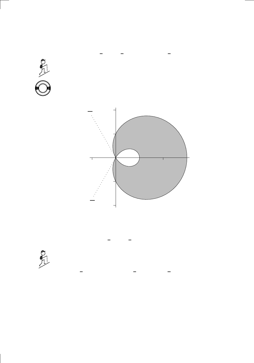
592 • Parametric Equations and Polar Coordinates
should be π(3/2)
2
, or 9π/4 square units. Let’s verify this. We have
area =
Z
π
0
1
2
r
2
dθ =
1
2
Z
π
0
(3 sin(θ))
2
dθ =
9
2
Z
π
0
sin
2
(θ) dθ.
This integral can be done using the double-angle formulas, as described at
PSfrag replacements
(
a, b)
[
a, b]
(
a, b]
[
a, b)
(
a, ∞)
[
a, ∞)
(
−∞, b)
(
−∞, b]
(
−∞, ∞)
{
x : a < x < b}
{
x : a ≤ x ≤ b}
{
x : a < x ≤ b}
{
x : a ≤ x < b}
{
x : x ≥ a}
{
x : x > a}
{
x : x ≤ b}
{
x : x < b}
R
a
b
shadow
0
1
4
−
2
3
−
3
g(
x) = x
2
f(
x) = x
3
g(
x) = x
2
f(
x) = x
3
mirror (
y = x)
f
−
1
(x) =
3
√
x
y = h
(x)
y = h
−
1
(x)
y = (
x − 1)
2
−
1
x
Same height
−
x
Same length,
opposite signs
y = −
2x
−
2
1
y =
1
2
x − 1
2
−
1
y = 2
x
y = 10
x
y = 2
−
x
y = log
2
(
x)
4
3 units
mirror (
x-axis)
y = |
x|
y = |
log
2
(x)|
θ radians
θ units
30
◦
=
π
6
45
◦
=
π
4
60
◦
=
π
3
120
◦
=
2
π
3
135
◦
=
3
π
4
150
◦
=
5
π
6
90
◦
=
π
2
180
◦
= π
210
◦
=
7
π
6
225
◦
=
5
π
4
240
◦
=
4
π
3
270
◦
=
3
π
2
300
◦
=
5
π
3
315
◦
=
7
π
4
330
◦
=
11
π
6
0
◦
= 0 radians
θ
hyp
otenuse
opposite
adjacent
0 (
≡ 2π)
π
2
π
3
π
2
I
II
III
IV
θ
(
x, y)
x
y
r
7
π
6
reference angle
reference angle =
π
6
sin +
sin −
cos +
cos −
tan +
tan −
A
S
T
C
7
π
4
9
π
13
5
π
6
(this angle is
5
π
6
clockwise)
1
2
1
2
3
4
5
6
0
−
1
−
2
−
3
−
4
−
5
−
6
−
3π
−
5
π
2
−
2π
−
3
π
2
−
π
−
π
2
3
π
3
π
5
π
2
2
π
3
π
2
π
π
2
y = sin(
x)
1
0
−
1
−
3π
−
5
π
2
−
2π
−
3
π
2
−
π
−
π
2
3
π
5
π
2
2
π
2
π
3
π
2
π
π
2
y = sin(
x)
y = cos(
x)
−
π
2
π
2
y = tan(
x), −
π
2
< x <
π
2
0
−
π
2
π
2
y = tan(
x)
−
2π
−
3π
−
5
π
2
−
3
π
2
−
π
−
π
2
π
2
3
π
3
π
5
π
2
2
π
3
π
2
π
y = sec(
x)
y = csc(
x)
y = cot(
x)
y = f(
x)
−
1
1
2
y = g(
x)
3
y = h
(x)
4
5
−
2
f(
x) =
1
x
g(
x) =
1
x
2
etc.
0
1
π
1
2
π
1
3
π
1
4
π
1
5
π
1
6
π
1
7
π
g(
x) = sin
1
x
1
0
−
1
L
10
100
200
y =
π
2
y = −
π
2
y = tan
−
1
(x)
π
2
π
y =
sin(
x)
x
, x > 3
0
1
−
1
a
L
f(
x) = x sin (1/x)
(0 < x < 0
.3)
h
(x) = x
g(
x) = −x
a
L
lim
x
→a
+
f(x) = L
lim
x
→a
+
f(x) = ∞
lim
x
→a
+
f(x) = −∞
lim
x
→a
+
f(x) DNE
lim
x
→a
−
f(x) = L
lim
x
→a
−
f(x) = ∞
lim
x
→a
−
f(x) = −∞
lim
x
→a
−
f(x) DNE
M
}
lim
x
→a
−
f(x) = M
lim
x
→a
f(x) = L
lim
x
→a
f(x) DNE
lim
x
→∞
f(x) = L
lim
x
→∞
f(x) = ∞
lim
x
→∞
f(x) = −∞
lim
x
→∞
f(x) DNE
lim
x
→−∞
f(x) = L
lim
x
→−∞
f(x) = ∞
lim
x
→−∞
f(x) = −∞
lim
x
→−∞
f(x) DNE
lim
x →a
+
f(
x) = ∞
lim
x →a
+
f(
x) = −∞
lim
x →a
−
f(
x) = ∞
lim
x →a
−
f(
x) = −∞
lim
x →a
f(
x) = ∞
lim
x →a
f(
x) = −∞
lim
x →a
f(
x) DNE
y = f (
x)
a
y =
|
x|
x
1
−
1
y =
|
x + 2|
x + 2
1
−
1
−
2
1
2
3
4
a
a
b
y = x sin
1
x
y = x
y = −
x
a
b
c
d
C
a
b
c
d
−
1
0
1
2
3
time
y
t
u
(
t, f(t))
(
u, f(u))
time
y
t
u
y
x
(
x, f(x))
y = |
x|
(
z, f(z))
z
y = f(
x)
a
tangent at x = a
b
tangent at x = b
c
tangent at x = c
y = x
2
tangent
at x = −
1
u
v
uv
u + ∆
u
v + ∆
v
(
u + ∆u)(v + ∆v)
∆
u
∆
v
u
∆v
v∆
u
∆
u∆v
y = f(
x)
1
2
−
2
y = |
x
2
− 4|
y = x
2
− 4
y = −
2x + 5
y = g(
x)
1
2
3
4
5
6
7
8
9
0
−
1
−
2
−
3
−
4
−
5
−
6
y = f (
x)
3
−
3
3
−
3
0
−
1
2
easy
hard
flat
y = f
0
(
x)
3
−
3
0
−
1
2
1
−
1
y = sin(
x)
y = x
x
A
B
O
1
C
D
sin(
x)
tan(
x)
y =
sin(
x)
x
π
2
π
1
−
1
x = 0
a = 0
x > 0
a > 0
x < 0
a < 0
rest position
+
−
y = x
2
sin
1
x
N
A
B
H
a
b
c
O
H
A
B
C
D
h
r
R
θ
1000
2000
α
β
p
h
y = g(
x) = log
b
(x)
y = f(
x) = b
x
y = e
x
5
10
1
2
3
4
0
−
1
−
2
−
3
−
4
y = ln(
x)
y = cosh(
x)
y = sinh(
x)
y = tanh(
x)
y = sech(
x)
y = csch(
x)
y = coth(
x)
1
−
1
y = f(
x)
original function
inverse function
slope = 0 at (
x, y)
slope is infinite at (
y, x)
−
108
2
5
1
2
1
2
3
4
5
6
0
−
1
−
2
−
3
−
4
−
5
−
6
−
3π
−
5
π
2
−
2π
−
3
π
2
−
π
−
π
2
3
π
3
π
5
π
2
2
π
3
π
2
π
π
2
y = sin(
x)
1
0
−
1
−
3π
−
5
π
2
−
2π
−
3
π
2
−
π
−
π
2
3
π
5
π
2
2
π
2
π
3
π
2
π
π
2
y = sin(
x)
y = sin(
x), −
π
2
≤ x ≤
π
2
−
2
−
1
0
2
π
2
−
π
2
y = sin
−
1
(x)
y = cos(
x)
π
π
2
y = cos
−
1
(x)
−
π
2
1
x
α
β
y = tan(
x)
y = tan(
x)
1
y = tan
−
1
(x)
y = sec(
x)
y = sec
−
1
(x)
y = csc
−
1
(x)
y = cot
−
1
(x)
1
y = cosh
−
1
(x)
y = sinh
−
1
(x)
y = tanh
−
1
(x)
y = sech
−
1
(x)
y = csch
−
1
(x)
y = coth
−
1
(x)
(0
, 3)
(2
, −1)
(5
, 2)
(7
, 0)
(
−1, 44)
(0
, 1)
(1
, −12)
(2
, 305)
y = 1
2
(2
, 3)
y = f(
x)
y = g(
x)
a
b
c
a
b
c
s
c
0
c
1
(
a, f(a))
(
b, f(b))
1
2
1
2
3
4
5
6
0
−
1
−
2
−
3
−
4
−
5
−
6
−
3π
−
5
π
2
−
2π
−
3
π
2
−
π
−
π
2
3
π
3
π
5
π
2
2
π
3
π
2
π
π
2
y = sin(
x)
1
0
−
1
−
3π
−
5
π
2
−
2π
−
3
π
2
−
π
−
π
2
3
π
5
π
2
2
π
2
π
3
π
2
π
π
2
c
OR
Local maximum
Local minimum
Horizontal point of inflection
1
e
y = f
0
(
x)
y = f (
x) = x ln(x)
−
1
e
?
y = f(
x) = x
3
y = g(
x) = x
4
x
f(
x)
−
3
−
2
−
1
0
1
2
1
2
3
4
+
−
?
1
5
6
3
f
0
(
x)
2 −
1
2
√
6
2 +
1
2
√
6
f
00
(
x)
7
8
g
00
(
x)
f
00
(
x)
0
y =
(
x − 3)(x − 1)
2
x
3
(
x + 2)
y = x ln(
x)
1
e
−
1
e
5
−
108
2
α
β
2 −
1
2
√
6
2 +
1
2
√
6
y = x
2
(
x − 5)
3
−
e
−
1/2
√
3
e
−
1/2
√
3
−
e
−3/2
e
−
3/2
−
1
√
3
1
√
3
−
1
1
y = xe
−
3x
2
/2
y =
x
3
− 6
x
2
+ 13x − 8
x
28
2
600
500
400
300
200
100
0
−
100
−
200
−
300
−
400
−
500
−
600
0
10
−
10
5
−
5
20
−
20
15
−
15
0
4
5
6
x
P
0
(
x)
+
−
−
existing fence
new fence
enclosure
A
h
b
H
99
100
101
h
dA/dh
r
h
1
2
7
shallow
deep
LAND
SEA
N
y
z
s
t
3
11
9
L
(11)
√
11
y = L
(x)
y = f (
x)
11
y = L
(x)
y = f(
x)
F
P
a
a + ∆
x
f(
a + ∆x)
L
(a + ∆x)
f(
a)
error
df
∆
x
a
b
y = f(
x)
true zero
starting approximation
better approximation
v
t
3
5
50
40
60
4
20
30
25
t
1
t
2
t
3
t
4
t
n
−2
t
n
−1
t
0
= a
t
n
= b
v
1
v
2
v
3
v
4
v
n
−1
v
n
−
30
6
30
|
v|
a
b
p
q
c
v(
c)
v(
c
1
)
v(
c
2
)
v(
c
3
)
v(
c
4
)
v(
c
5
)
v(
c
6
)
t
1
t
2
t
3
t
4
t
5
c
1
c
2
c
3
c
4
c
5
c
6
t
0
=
a
t
6
=
b
t
16
=
b
t
10
=
b
a
b
x
y
y = f(
x)
1
2
y = x
5
0
−
2
y = 1
a
b
y = sin(
x)
π
−
π
0
−
1
−
2
0
2
4
y = x
2
0
1
2
3
4
2
n
4
n
6
n
2(
n−2)
n
2(
n−1)
n
2
n
n
= 2
width of each interval =
2
n
−
2
1
3
0
I
II
III
IV
4
y
dx
y = −
x
2
− 2x + 3
3
−
5
y = |−
x
2
− 2x + 3|
I
II
IIa
5
3
0
1
2
a
b
y = f (
x)
y = g(
x)
y = x
2
a
b
5
3
0
1
2
y =
√
x
2
√
2
2
2
dy
x
2
a
b
y = f(
x)
y = g(
x)
M
m
1
2
−
1
−
2
0
y = e
−
x
2
1
2
e
−
1/4
f
av
y = f
av
c
A
M
0
1
2
a
b
x
t
y = f (
t)
F (
x )
y = f (
t)
F (
x + h)
x + h
F (
x + h) − F (x)
f(
x)
1
2
y = sin(
x)
π
−
π
−
1
−
2
y =
1
x
y = x
2
1
2
1
−
1
y = ln
|x|
θ
a
x
a
x
p
a
2
− x
2
3
x
p
9 − x
2
p
x
2
+ a
2
x
a
p
x
2
+ 15
x
√
15
x
p
x
2
− a
2
a
x
p
x
2
− 4
2
x
−
p
x
2
− a
2
a
x
−
p
x
2
− 4
2
y = f(
x)
a
b
a + ε
ε
Z
b
a
+ε
f(x) dx
small
even smaller
y = g(
x)
infinite area
finite area
1
y =
1
x
y =
1
x
p
, p < 1 (typical)
y =
1
x
p
, p > 1 (typical)
a
1
a
2
a
3
a
4
a
5
a
6
a
7
a
8
1
2
3
4
5
6
7
8
n
a
n
x
y
y = f(
x)
(
a, f(a))
a
−
1
0
1
a
6
1
2
7
1
2
7
?
−
2
−
1
−
2
t = 0
t = π/
6
t = π/
4
t = π/
3
t = π/
2
3
0
t = −
2
t = −
3/2
t = ±
1
t = −
1/2
t = 0
t = 1
/2
t = 3
/2
t = 2
12
−
12
θ
r
P
θ
r
P
11π
6
2
(−1, −1)
wrong point
π
4
5π
4
√
2
(0, 1)
(0, −3)
(−2, 0)
π
2
3π
2
π
r = 3 sin(θ)
3π
2
θ
2π
1
0
−1
−2
−3
0
3
2
−
3
2
0
r = 1 + 2 cos(θ)
2π
3
4π
3
0
π
0
pi
−
3
2
3π
2
1
2
3
0
−1
−2
−3
0 ≤ θ ≤
2π
3
0 ≤ θ ≤ π
0 ≤ θ ≤ 2π
r = 1 + cos(θ)
r = 1 +
3
4
cos(θ)
−
1
4
r = sin(2θ)
r = sin(3θ)
r =
1
π
θ
0 ≤ θ ≤ 4π
r =
2
1 + sin(θ)
−
π
4
≤ θ ≤
5π
4
0 ≤ θ ≤ 2π
0 ≤ θ ≤ π
−4
−5
4
5
f(θ)
f(θ + dθ)
θ
dθ
θ + dθ
approximating region
exact region
the beginning of Section 19.1 in Chapter 19. Check that you agree that the
answer is 9π/4.
Here’s a harder example. Let’s try to find the area of the croissant-shaped
PSfrag replacements
(
a, b)
[
a, b]
(
a, b]
[
a, b)
(
a, ∞)
[
a, ∞)
(
−∞, b)
(
−∞, b]
(
−∞, ∞)
{
x : a < x < b}
{
x : a ≤ x ≤ b}
{
x : a < x ≤ b}
{
x : a ≤ x < b}
{
x : x ≥ a}
{
x : x > a}
{
x : x ≤ b}
{
x : x < b}
R
a
b
shadow
0
1
4
−
2
3
−
3
g(
x) = x
2
f(
x) = x
3
g(
x) = x
2
f(
x) = x
3
mirror (
y = x)
f
−
1
(x) =
3
√
x
y = h
(x)
y = h
−
1
(x)
y = (
x − 1)
2
−
1
x
Same height
−
x
Same length,
opposite signs
y = −
2x
−
2
1
y =
1
2
x − 1
2
−
1
y = 2
x
y = 10
x
y = 2
−
x
y = log
2
(
x)
4
3 units
mirror (
x-axis)
y = |
x|
y = |
log
2
(x)|
θ radians
θ units
30
◦
=
π
6
45
◦
=
π
4
60
◦
=
π
3
120
◦
=
2
π
3
135
◦
=
3
π
4
150
◦
=
5
π
6
90
◦
=
π
2
180
◦
= π
210
◦
=
7
π
6
225
◦
=
5
π
4
240
◦
=
4
π
3
270
◦
=
3
π
2
300
◦
=
5
π
3
315
◦
=
7
π
4
330
◦
=
11
π
6
0
◦
= 0 radians
θ
hyp
otenuse
opposite
adjacent
0 (
≡ 2π)
π
2
π
3
π
2
I
II
III
IV
θ
(
x, y)
x
y
r
7
π
6
reference angle
reference angle =
π
6
sin +
sin −
cos +
cos −
tan +
tan −
A
S
T
C
7
π
4
9
π
13
5
π
6
(this angle is
5
π
6
clockwise)
1
2
1
2
3
4
5
6
0
−
1
−
2
−
3
−
4
−
5
−
6
−
3π
−
5
π
2
−
2π
−
3
π
2
−
π
−
π
2
3
π
3
π
5
π
2
2
π
3
π
2
π
π
2
y = sin(
x)
1
0
−
1
−
3π
−
5
π
2
−
2π
−
3
π
2
−
π
−
π
2
3
π
5
π
2
2
π
2
π
3
π
2
π
π
2
y = sin(
x)
y = cos(
x)
−
π
2
π
2
y = tan(
x), −
π
2
< x <
π
2
0
−
π
2
π
2
y = tan(
x)
−
2π
−
3π
−
5
π
2
−
3
π
2
−
π
−
π
2
π
2
3
π
3
π
5
π
2
2
π
3
π
2
π
y = sec(
x)
y = csc(
x)
y = cot(
x)
y = f(
x)
−
1
1
2
y = g(
x)
3
y = h
(x)
4
5
−
2
f(
x) =
1
x
g(
x) =
1
x
2
etc.
0
1
π
1
2
π
1
3
π
1
4
π
1
5
π
1
6
π
1
7
π
g(
x) = sin
1
x
1
0
−
1
L
10
100
200
y =
π
2
y = −
π
2
y = tan
−
1
(x)
π
2
π
y =
sin(
x)
x
, x > 3
0
1
−
1
a
L
f(
x) = x sin (1/x)
(0 < x < 0
.3)
h
(x) = x
g(
x) = −x
a
L
lim
x
→a
+
f(x) = L
lim
x
→a
+
f(x) = ∞
lim
x
→a
+
f(x) = −∞
lim
x
→a
+
f(x) DNE
lim
x
→a
−
f(x) = L
lim
x
→a
−
f(x) = ∞
lim
x
→a
−
f(x) = −∞
lim
x
→a
−
f(x) DNE
M
}
lim
x
→a
−
f(x) = M
lim
x
→a
f(x) = L
lim
x
→a
f(x) DNE
lim
x
→∞
f(x) = L
lim
x
→∞
f(x) = ∞
lim
x
→∞
f(x) = −∞
lim
x
→∞
f(x) DNE
lim
x
→−∞
f(x) = L
lim
x
→−∞
f(x) = ∞
lim
x
→−∞
f(x) = −∞
lim
x
→−∞
f(x) DNE
lim
x →a
+
f(
x) = ∞
lim
x →a
+
f(
x) = −∞
lim
x →a
−
f(
x) = ∞
lim
x →a
−
f(
x) = −∞
lim
x →a
f(
x) = ∞
lim
x →a
f(
x) = −∞
lim
x →a
f(
x) DNE
y = f (
x)
a
y =
|
x|
x
1
−
1
y =
|
x + 2|
x + 2
1
−
1
−
2
1
2
3
4
a
a
b
y = x sin
1
x
y = x
y = −
x
a
b
c
d
C
a
b
c
d
−
1
0
1
2
3
time
y
t
u
(
t, f(t))
(
u, f(u))
time
y
t
u
y
x
(
x, f(x))
y = |
x|
(
z, f(z))
z
y = f(
x)
a
tangent at x = a
b
tangent at x = b
c
tangent at x = c
y = x
2
tangent
at x = −
1
u
v
uv
u + ∆
u
v + ∆
v
(
u + ∆u)(v + ∆v)
∆
u
∆
v
u
∆v
v∆
u
∆
u∆v
y = f(
x)
1
2
−
2
y = |
x
2
− 4|
y = x
2
− 4
y = −
2x + 5
y = g(
x)
1
2
3
4
5
6
7
8
9
0
−
1
−
2
−
3
−
4
−
5
−
6
y = f (
x)
3
−
3
3
−
3
0
−
1
2
easy
hard
flat
y = f
0
(
x)
3
−
3
0
−
1
2
1
−
1
y = sin(
x)
y = x
x
A
B
O
1
C
D
sin(
x)
tan(
x)
y =
sin(
x)
x
π
2
π
1
−
1
x = 0
a = 0
x > 0
a > 0
x < 0
a < 0
rest position
+
−
y = x
2
sin
1
x
N
A
B
H
a
b
c
O
H
A
B
C
D
h
r
R
θ
1000
2000
α
β
p
h
y = g(
x) = log
b
(x)
y = f(
x) = b
x
y = e
x
5
10
1
2
3
4
0
−
1
−
2
−
3
−
4
y = ln(
x)
y = cosh(
x)
y = sinh(
x)
y = tanh(
x)
y = sech(
x)
y = csch(
x)
y = coth(
x)
1
−
1
y = f(
x)
original function
inverse function
slope = 0 at (
x, y)
slope is infinite at (
y, x)
−
108
2
5
1
2
1
2
3
4
5
6
0
−
1
−
2
−
3
−
4
−
5
−
6
−
3π
−
5
π
2
−
2π
−
3
π
2
−
π
−
π
2
3
π
3
π
5
π
2
2
π
3
π
2
π
π
2
y = sin(
x)
1
0
−
1
−
3π
−
5
π
2
−
2π
−
3
π
2
−
π
−
π
2
3
π
5
π
2
2
π
2
π
3
π
2
π
π
2
y = sin(
x)
y = sin(
x), −
π
2
≤ x ≤
π
2
−
2
−
1
0
2
π
2
−
π
2
y = sin
−
1
(x)
y = cos(
x)
π
π
2
y = cos
−
1
(x)
−
π
2
1
x
α
β
y = tan(
x)
y = tan(
x)
1
y = tan
−
1
(x)
y = sec(
x)
y = sec
−
1
(x)
y = csc
−
1
(x)
y = cot
−
1
(x)
1
y = cosh
−
1
(x)
y = sinh
−
1
(x)
y = tanh
−
1
(x)
y = sech
−
1
(x)
y = csch
−
1
(x)
y = coth
−
1
(x)
(0
, 3)
(2
, −1)
(5
, 2)
(7
, 0)
(
−1, 44)
(0
, 1)
(1
, −12)
(2
, 305)
y = 1
2
(2
, 3)
y = f(
x)
y = g(
x)
a
b
c
a
b
c
s
c
0
c
1
(
a, f(a))
(
b, f(b))
1
2
1
2
3
4
5
6
0
−
1
−
2
−
3
−
4
−
5
−
6
−
3π
−
5
π
2
−
2π
−
3
π
2
−
π
−
π
2
3
π
3
π
5
π
2
2
π
3
π
2
π
π
2
y = sin(
x)
1
0
−
1
−
3π
−
5
π
2
−
2π
−
3
π
2
−
π
−
π
2
3
π
5
π
2
2
π
2
π
3
π
2
π
π
2
c
OR
Local maximum
Local minimum
Horizontal point of inflection
1
e
y = f
0
(
x)
y = f (
x) = x ln(x)
−
1
e
?
y = f(
x) = x
3
y = g(
x) = x
4
x
f(
x)
−
3
−
2
−
1
0
1
2
1
2
3
4
+
−
?
1
5
6
3
f
0
(
x)
2 −
1
2
√
6
2 +
1
2
√
6
f
00
(
x)
7
8
g
00
(
x)
f
00
(
x)
0
y =
(
x − 3)(x − 1)
2
x
3
(
x + 2)
y = x ln(
x)
1
e
−
1
e
5
−
108
2
α
β
2 −
1
2
√
6
2 +
1
2
√
6
y = x
2
(
x − 5)
3
−
e
−
1/2
√
3
e
−
1/2
√
3
−
e
−3/2
e
−
3/2
−
1
√
3
1
√
3
−
1
1
y = xe
−
3x
2
/2
y =
x
3
− 6
x
2
+ 13x − 8
x
28
2
600
500
400
300
200
100
0
−
100
−
200
−
300
−
400
−
500
−
600
0
10
−
10
5
−
5
20
−
20
15
−
15
0
4
5
6
x
P
0
(
x)
+
−
−
existing fence
new fence
enclosure
A
h
b
H
99
100
101
h
dA/dh
r
h
1
2
7
shallow
deep
LAND
SEA
N
y
z
s
t
3
11
9
L
(11)
√
11
y = L
(x)
y = f (
x)
11
y = L
(x)
y = f(
x)
F
P
a
a + ∆
x
f(
a + ∆x)
L
(a + ∆x)
f(
a)
error
df
∆
x
a
b
y = f(
x)
true zero
starting approximation
better approximation
v
t
3
5
50
40
60
4
20
30
25
t
1
t
2
t
3
t
4
t
n
−2
t
n
−1
t
0
= a
t
n
= b
v
1
v
2
v
3
v
4
v
n
−1
v
n
−
30
6
30
|
v|
a
b
p
q
c
v(
c)
v(
c
1
)
v(
c
2
)
v(
c
3
)
v(
c
4
)
v(
c
5
)
v(
c
6
)
t
1
t
2
t
3
t
4
t
5
c
1
c
2
c
3
c
4
c
5
c
6
t
0
=
a
t
6
=
b
t
16
=
b
t
10
=
b
a
b
x
y
y = f(
x)
1
2
y = x
5
0
−
2
y = 1
a
b
y = sin(
x)
π
−
π
0
−
1
−
2
0
2
4
y = x
2
0
1
2
3
4
2
n
4
n
6
n
2(
n−2)
n
2(
n−1)
n
2
n
n
= 2
width of each interval =
2
n
−
2
1
3
0
I
II
III
IV
4
y
dx
y = −
x
2
− 2x + 3
3
−
5
y = |−
x
2
− 2x + 3|
I
II
IIa
5
3
0
1
2
a
b
y = f (
x)
y = g(
x)
y = x
2
a
b
5
3
0
1
2
y =
√
x
2
√
2
2
2
dy
x
2
a
b
y = f(
x)
y = g(
x)
M
m
1
2
−
1
−
2
0
y = e
−
x
2
1
2
e
−
1/4
f
av
y = f
av
c
A
M
0
1
2
a
b
x
t
y = f (
t)
F (
x )
y = f (
t)
F (
x + h)
x + h
F (
x + h) − F (x)
f(
x)
1
2
y = sin(
x)
π
−
π
−
1
−
2
y =
1
x
y = x
2
1
2
1
−
1
y = ln
|x|
θ
a
x
a
x
p
a
2
− x
2
3
x
p
9 − x
2
p
x
2
+ a
2
x
a
p
x
2
+ 15
x
√
15
x
p
x
2
− a
2
a
x
p
x
2
− 4
2
x
−
p
x
2
− a
2
a
x
−
p
x
2
− 4
2
y = f(
x)
a
b
a + ε
ε
Z
b
a
+ε
f(x) dx
small
even smaller
y = g(
x)
infinite area
finite area
1
y =
1
x
y =
1
x
p
, p < 1 (typical)
y =
1
x
p
, p > 1 (typical)
a
1
a
2
a
3
a
4
a
5
a
6
a
7
a
8
1
2
3
4
5
6
7
8
n
a
n
x
y
y = f(
x)
(
a, f(a))
a
−
1
0
1
a
6
1
2
7
1
2
7
?
−
2
−
1
−
2
t = 0
t = π/
6
t = π/
4
t = π/
3
t = π/
2
3
0
t = −
2
t = −
3/2
t = ±
1
t = −
1/2
t = 0
t = 1
/2
t = 3
/2
t = 2
12
−
12
θ
r
P
θ
r
P
11π
6
2
(−1, −1)
wrong point
π
4
5π
4
√
2
(0, 1)
(0, −3)
(−2, 0)
π
2
3π
2
π
r = 3 sin(θ)
3π
2
θ
2π
1
0
−1
−2
−3
0
3
2
−
3
2
0
r = 1 + 2 cos(θ)
2π
3
4π
3
0
π
0
pi
−
3
2
3π
2
1
2
3
0
−1
−2
−3
0 ≤ θ ≤
2π
3
0 ≤ θ ≤ π
0 ≤ θ ≤ 2π
r = 1 + cos(θ)
r = 1 +
3
4
cos(θ)
−
1
4
r = sin(2θ)
r = sin(3θ)
r =
1
π
θ
0 ≤ θ ≤ 4π
r =
2
1 + sin(θ)
−
π
4
≤ θ ≤
5π
4
0 ≤ θ ≤ 2π
0 ≤ θ ≤ π
−4
−5
4
5
f(θ)
f(θ + dθ)
θ
dθ
θ + dθ
approximating region
exact region
region enclosed by our curve r = 1 + 2 cos(θ), as shown in the following
diagram:
PSfrag replacements
(
a, b)
[
a, b]
(
a, b]
[
a, b)
(
a, ∞)
[
a, ∞)
(
−∞, b)
(
−∞, b]
(
−∞, ∞)
{
x : a < x < b}
{
x : a ≤ x ≤ b}
{
x : a < x ≤ b}
{
x : a ≤ x < b}
{
x : x ≥ a}
{
x : x > a}
{
x : x ≤ b}
{
x : x < b}
R
a
b
shadow
0
1
4
−
2
3
−
3
g(
x) = x
2
f(
x) = x
3
g(
x) = x
2
f(
x) = x
3
mirror (
y = x)
f
−
1
(x) =
3
√
x
y = h
(x)
y = h
−
1
(x)
y = (
x − 1)
2
−
1
x
Same height
−
x
Same length,
opposite signs
y = −
2x
−
2
1
y =
1
2
x − 1
2
−
1
y = 2
x
y = 10
x
y = 2
−
x
y = log
2
(
x)
4
3 units
mirror (
x-axis)
y = |
x|
y = |
log
2
(x)|
θ radians
θ units
30
◦
=
π
6
45
◦
=
π
4
60
◦
=
π
3
120
◦
=
2
π
3
135
◦
=
3
π
4
150
◦
=
5
π
6
90
◦
=
π
2
180
◦
= π
210
◦
=
7
π
6
225
◦
=
5
π
4
240
◦
=
4
π
3
270
◦
=
3
π
2
300
◦
=
5
π
3
315
◦
=
7
π
4
330
◦
=
11
π
6
0
◦
= 0 radians
θ
hyp
otenuse
opposite
adjacent
0 (
≡ 2π)
π
2
π
3
π
2
I
II
III
IV
θ
(
x, y)
x
y
r
7
π
6
reference angle
reference angle =
π
6
sin +
sin −
cos +
cos −
tan +
tan −
A
S
T
C
7
π
4
9
π
13
5
π
6
(this angle is
5
π
6
clockwise)
1
2
1
2
3
4
5
6
0
−
1
−
2
−
3
−
4
−
5
−
6
−
3π
−
5
π
2
−
2π
−
3
π
2
−
π
−
π
2
3
π
3
π
5
π
2
2
π
3
π
2
π
π
2
y = sin(
x)
1
0
−
1
−
3π
−
5
π
2
−
2π
−
3
π
2
−
π
−
π
2
3
π
5
π
2
2
π
2
π
3
π
2
π
π
2
y = sin(
x)
y = cos(
x)
−
π
2
π
2
y = tan(
x), −
π
2
< x <
π
2
0
−
π
2
π
2
y = tan(
x)
−
2π
−
3π
−
5
π
2
−
3
π
2
−
π
−
π
2
π
2
3
π
3
π
5
π
2
2
π
3
π
2
π
y = sec(
x)
y = csc(
x)
y = cot(
x)
y = f(
x)
−
1
1
2
y = g(
x)
3
y = h
(x)
4
5
−
2
f(
x) =
1
x
g(
x) =
1
x
2
etc.
0
1
π
1
2
π
1
3
π
1
4
π
1
5
π
1
6
π
1
7
π
g(
x) = sin
1
x
1
0
−
1
L
10
100
200
y =
π
2
y = −
π
2
y = tan
−
1
(x)
π
2
π
y =
sin(
x)
x
, x > 3
0
1
−
1
a
L
f(
x) = x sin (1/x)
(0 < x < 0
.3)
h
(x) = x
g(
x) = −x
a
L
lim
x
→a
+
f(x) = L
lim
x
→a
+
f(x) = ∞
lim
x
→a
+
f(x) = −∞
lim
x
→a
+
f(x) DNE
lim
x
→a
−
f(x) = L
lim
x
→a
−
f(x) = ∞
lim
x
→a
−
f(x) = −∞
lim
x
→a
−
f(x) DNE
M
}
lim
x
→a
−
f(x) = M
lim
x
→a
f(x) = L
lim
x
→a
f(x) DNE
lim
x
→∞
f(x) = L
lim
x
→∞
f(x) = ∞
lim
x
→∞
f(x) = −∞
lim
x
→∞
f(x) DNE
lim
x
→−∞
f(x) = L
lim
x
→−∞
f(x) = ∞
lim
x
→−∞
f(x) = −∞
lim
x
→−∞
f(x) DNE
lim
x →a
+
f(
x) = ∞
lim
x →a
+
f(
x) = −∞
lim
x →a
−
f(
x) = ∞
lim
x →a
−
f(
x) = −∞
lim
x →a
f(
x) = ∞
lim
x →a
f(
x) = −∞
lim
x →a
f(
x) DNE
y = f (
x)
a
y =
|
x|
x
1
−
1
y =
|
x + 2|
x + 2
1
−
1
−
2
1
2
3
4
a
a
b
y = x sin
1
x
y = x
y = −
x
a
b
c
d
C
a
b
c
d
−
1
0
1
2
3
time
y
t
u
(
t, f(t))
(
u, f(u))
time
y
t
u
y
x
(
x, f(x))
y = |
x|
(
z, f(z))
z
y = f(
x)
a
tangent at x = a
b
tangent at x = b
c
tangent at x = c
y = x
2
tangent
at x = −
1
u
v
uv
u + ∆
u
v + ∆
v
(
u + ∆u)(v + ∆v)
∆
u
∆
v
u
∆v
v∆
u
∆
u∆v
y = f(
x)
1
2
−
2
y = |
x
2
− 4|
y = x
2
− 4
y = −
2x + 5
y = g(
x)
1
2
3
4
5
6
7
8
9
0
−
1
−
2
−
3
−
4
−
5
−
6
y = f(
x)
3
−
3
3
−
3
0
−
1
2
easy
hard
flat
y = f
0
(
x)
3
−
3
0
−
1
2
1
−
1
y = sin(
x)
y = x
x
A
B
O
1
C
D
sin(
x)
tan(
x)
y =
sin(
x)
x
π
2
π
1
−
1
x = 0
a = 0
x > 0
a > 0
x < 0
a < 0
rest position
+
−
y = x
2
sin
1
x
N
A
B
H
a
b
c
O
H
A
B
C
D
h
r
R
θ
1000
2000
α
β
p
h
y = g(
x) = log
b
(x)
y = f (
x) = b
x
y = e
x
5
10
1
2
3
4
0
−
1
−
2
−
3
−
4
y = ln(
x)
y = cosh(
x)
y = sinh(
x)
y = tanh(
x)
y = sech(
x)
y = csch(
x)
y = coth(
x)
1
−
1
y = f(
x)
original function
inverse function
slope = 0 at (
x, y)
slope is infinite at (
y, x)
−
108
2
5
1
2
1
2
3
4
5
6
0
−
1
−
2
−
3
−
4
−
5
−
6
−
3π
−
5
π
2
−
2π
−
3
π
2
−
π
−
π
2
3
π
3
π
5
π
2
2
π
3
π
2
π
π
2
y = sin(
x)
1
0
−
1
−
3π
−
5
π
2
−
2π
−
3
π
2
−
π
−
π
2
3
π
5
π
2
2
π
2
π
3
π
2
π
π
2
y = sin(
x)
y = sin(
x), −
π
2
≤ x ≤
π
2
−
2
−
1
0
2
π
2
−
π
2
y = sin
−
1
(x)
y = cos(
x)
π
π
2
y = cos
−
1
(x)
−
π
2
1
x
α
β
y = tan(
x)
y = tan(
x)
1
y = tan
−
1
(x)
y = sec(
x)
y = sec
−
1
(x)
y = csc
−
1
(x)
y = cot
−
1
(x)
1
y = cosh
−
1
(x)
y = sinh
−
1
(x)
y = tanh
−
1
(x)
y = sech
−
1
(x)
y = csch
−
1
(x)
y = coth
−
1
(x)
(0
, 3)
(2
, −1)
(5
, 2)
(7
, 0)
(
−1, 44)
(0
, 1)
(1
, −12)
(2
, 305)
y = 1
2
(2
, 3)
y = f(
x)
y = g(
x)
a
b
c
a
b
c
s
c
0
c
1
(
a, f(a))
(
b, f(b))
1
2
1
2
3
4
5
6
0
−
1
−
2
−
3
−
4
−
5
−
6
−
3π
−
5
π
2
−
2π
−
3
π
2
−
π
−
π
2
3
π
3
π
5
π
2
2
π
3
π
2
π
π
2
y = sin(
x)
1
0
−
1
−
3π
−
5
π
2
−
2π
−
3
π
2
−
π
−
π
2
3
π
5
π
2
2
π
2
π
3
π
2
π
π
2
c
OR
Local maximum
Local minimum
Horizontal point of inflection
1
e
y = f
0
(
x)
y = f(
x) = x ln(x)
−
1
e
?
y = f (
x) = x
3
y = g(
x) = x
4
x
f(
x)
−
3
−
2
−
1
0
1
2
1
2
3
4
+
−
?
1
5
6
3
f
0
(
x)
2 −
1
2
√
6
2 +
1
2
√
6
f
00
(
x)
7
8
g
00
(
x)
f
00
(
x)
0
y =
(
x − 3)(x − 1)
2
x
3
(
x + 2)
y = x ln(
x)
1
e
−
1
e
5
−
108
2
α
β
2 −
1
2
√
6
2 +
1
2
√
6
y = x
2
(
x − 5)
3
−
e
−
1/2
√
3
e
−
1/2
√
3
−
e
−3/2
e
−
3/2
−
1
√
3
1
√
3
−
1
1
y = xe
−
3x
2
/2
y =
x
3
− 6
x
2
+ 13x − 8
x
28
2
600
500
400
300
200
100
0
−
100
−
200
−
300
−
400
−
500
−
600
0
10
−
10
5
−
5
20
−
20
15
−
15
0
4
5
6
x
P
0
(
x)
+
−
−
existing fence
new fence
enclosure
A
h
b
H
99
100
101
h
dA/dh
r
h
1
2
7
shallow
deep
LAND
SEA
N
y
z
s
t
3
11
9
L
(11)
√
11
y = L
(x)
y = f(
x)
11
y = L
(x)
y = f(
x)
F
P
a
a + ∆
x
f(
a + ∆x)
L
(a + ∆x)
f(
a)
error
df
∆
x
a
b
y = f(
x)
true zero
starting approximation
better approximation
v
t
3
5
50
40
60
4
20
30
25
t
1
t
2
t
3
t
4
t
n
−2
t
n
−1
t
0
= a
t
n
= b
v
1
v
2
v
3
v
4
v
n
−1
v
n
−
30
6
30
|
v|
a
b
p
q
c
v(
c)
v(
c
1
)
v(
c
2
)
v(
c
3
)
v(
c
4
)
v(
c
5
)
v(
c
6
)
t
1
t
2
t
3
t
4
t
5
c
1
c
2
c
3
c
4
c
5
c
6
t
0
=
a
t
6
=
b
t
16
=
b
t
10
=
b
a
b
x
y
y = f(
x)
1
2
y = x
5
0
−
2
y = 1
a
b
y = sin(
x)
π
−
π
0
−
1
−
2
0
2
4
y = x
2
0
1
2
3
4
2
n
4
n
6
n
2(
n−2)
n
2(
n−1)
n
2
n
n
= 2
width of each interval =
2
n
−
2
1
3
0
I
II
III
IV
4
y
dx
y = −
x
2
− 2x + 3
3
−
5
y = |−
x
2
− 2x + 3|
I
II
IIa
5
3
0
1
2
a
b
y = f(
x)
y = g(
x)
y = x
2
a
b
5
3
0
1
2
y =
√
x
2
√
2
2
2
dy
x
2
a
b
y = f(
x)
y = g(
x)
M
m
1
2
−
1
−
2
0
y = e
−
x
2
1
2
e
−
1/4
f
av
y = f
av
c
A
M
0
1
2
a
b
x
t
y = f(
t)
F (
x )
y = f(
t)
F (
x + h )
x + h
F (
x + h) − F (x)
f(
x)
1
2
y = sin(
x)
π
−
π
−
1
−
2
y =
1
x
y = x
2
1
2
1
−
1
y = ln|
x|
θ
a
x
a
x
p
a
2
− x
2
3
x
p
9 − x
2
p
x
2
+ a
2
x
a
p
x
2
+ 15
x
√
15
x
p
x
2
− a
2
a
x
p
x
2
− 4
2
x
−
p
x
2
− a
2
a
x
−
p
x
2
− 4
2
y = f(
x)
a
b
a + ε
ε
Z
b
a
+ε
f(x) dx
small
even smaller
y = g(
x)
infinite area
finite area
1
y =
1
x
y =
1
x
p
, p < 1 (typical)
y =
1
x
p
, p > 1 (typical)
a
1
a
2
a
3
a
4
a
5
a
6
a
7
a
8
1
2
3
4
5
6
7
8
n
a
n
x
y
y = f(
x)
(
a, f(a))
a
−
1
0
1
a
6
1
2
7
1
2
7
?
−
2
−
1
−
2
t = 0
t = π/6
t = π/4
t = π/3
t = π/2
3
0
t = −2
t = −3/2
t = ±1
t = −1/2
t = 0
t = 1/2
t = 3/2
t = 2
12
−12
θ
r
P
θ
r
P
11π
6
2
(−1, −1)
wrong point
π
4
5π
4
√
2
(0, 1)
(0, −3)
(−2, 0)
π
2
3π
2
π
r = 3 sin(θ)
3π
2
θ
2π
1
0
−1
−2
−3
0
3
2
−
3
2
0
r = 1 + 2 cos(θ)
2π
3
4π
3
0
π
0
pi
−
3
2
3π
2
1
1
2
2
3
0
−1
−1
−2
−3
0 ≤ θ ≤
2π
3
0 ≤ θ ≤ π
0 ≤ θ ≤ 2π
r = 1 + cos(θ)
r = 1 +
3
4
cos(θ)
−
1
4
r = sin(2θ)
r = sin(3θ)
r =
1
π
θ
0 ≤ θ ≤ 4π
r =
2
1 + sin(θ)
−
π
4
≤ θ ≤
5π
4
0 ≤ θ ≤ 2π
0 ≤ θ ≤ π
−4
−5
4
5
f(θ)
f(θ + dθ)
θ
dθ
θ + dθ
approximating region
exact region
0 ≤ θ ≤ 2π
It seems as if we should just be able to use the formula to say that the area
we want is given by
Z
2π
0
1
2
r
2
dθ =
1
2
Z
2π
0
(1 + 2 cos(θ))
2
dθ.
Again, to do this integral we need the double-angle formulas. I leave it to you
to show that
PSfrag replacements
(
a, b)
[
a, b]
(
a, b]
[
a, b)
(
a, ∞)
[
a, ∞)
(
−∞, b)
(
−∞, b]
(
−∞, ∞)
{
x : a < x < b}
{
x : a ≤ x ≤ b}
{
x : a < x ≤ b}
{
x : a ≤ x < b}
{
x : x ≥ a}
{
x : x > a}
{
x : x ≤ b}
{
x : x < b}
R
a
b
shadow
0
1
4
−
2
3
−
3
g(
x) = x
2
f(
x) = x
3
g(
x) = x
2
f(
x) = x
3
mirror (
y = x)
f
−
1
(x) =
3
√
x
y = h
(x)
y = h
−
1
(x)
y = (
x − 1)
2
−
1
x
Same height
−
x
Same length,
opposite signs
y = −
2x
−
2
1
y =
1
2
x − 1
2
−
1
y = 2
x
y = 10
x
y = 2
−
x
y = log
2
(
x)
4
3 units
mirror (
x-axis)
y = |
x|
y = |
log
2
(x)|
θ radians
θ units
30
◦
=
π
6
45
◦
=
π
4
60
◦
=
π
3
120
◦
=
2
π
3
135
◦
=
3
π
4
150
◦
=
5
π
6
90
◦
=
π
2
180
◦
= π
210
◦
=
7
π
6
225
◦
=
5
π
4
240
◦
=
4
π
3
270
◦
=
3
π
2
300
◦
=
5
π
3
315
◦
=
7
π
4
330
◦
=
11
π
6
0
◦
= 0 radians
θ
hyp
oten
use
opposite
adjacent
0 (
≡ 2π)
π
2
π
3
π
2
I
II
III
IV
θ
(
x, y)
x
y
r
7
π
6
reference angle
reference angle =
π
6
sin +
sin −
cos +
cos −
tan +
tan −
A
S
T
C
7
π
4
9
π
13
5
π
6
(this angle is
5
π
6
clockwise)
1
2
1
2
3
4
5
6
0
−
1
−
2
−
3
−
4
−
5
−
6
−
3π
−
5
π
2
−
2π
−
3
π
2
−
π
−
π
2
3
π
3
π
5
π
2
2
π
3
π
2
π
π
2
y = sin(
x)
1
0
−
1
−
3π
−
5
π
2
−
2π
−
3
π
2
−
π
−
π
2
3
π
5
π
2
2
π
2
π
3
π
2
π
π
2
y = sin(
x)
y = cos(
x)
−
π
2
π
2
y = tan(
x), −
π
2
< x <
π
2
0
−
π
2
π
2
y = tan(
x)
−
2π
−
3π
−
5
π
2
−
3
π
2
−
π
−
π
2
π
2
3
π
3
π
5
π
2
2
π
3
π
2
π
y = sec(
x)
y = csc(
x)
y = cot(
x)
y = f(
x)
−
1
1
2
y = g(
x)
3
y = h
(x)
4
5
−
2
f(
x) =
1
x
g(
x) =
1
x
2
etc.
0
1
π
1
2
π
1
3
π
1
4
π
1
5
π
1
6
π
1
7
π
g(
x) = sin
1
x
1
0
−
1
L
10
100
200
y =
π
2
y = −
π
2
y = tan
−
1
(x)
π
2
π
y =
sin(
x)
x
, x > 3
0
1
−
1
a
L
f(
x) = x sin (1/x)
(0 < x < 0
.3)
h
(x) = x
g(
x) = −x
a
L
lim
x
→a
+
f(x) = L
lim
x
→a
+
f(x) = ∞
lim
x
→a
+
f(x) = −∞
lim
x
→a
+
f(x) DNE
lim
x
→a
−
f(x) = L
lim
x
→a
−
f(x) = ∞
lim
x
→a
−
f(x) = −∞
lim
x
→a
−
f(x) DNE
M
}
lim
x
→a
−
f(x) = M
lim
x
→a
f(x) = L
lim
x
→a
f(x) DNE
lim
x
→∞
f(x) = L
lim
x
→∞
f(x) = ∞
lim
x
→∞
f(x) = −∞
lim
x
→∞
f(x) DNE
lim
x
→−∞
f(x) = L
lim
x
→−∞
f(x) = ∞
lim
x
→−∞
f(x) = −∞
lim
x
→−∞
f(x) DNE
lim
x →a
+
f(
x) = ∞
lim
x →a
+
f(
x) = −∞
lim
x →a
−
f(
x) = ∞
lim
x →a
−
f(
x) = −∞
lim
x →a
f(
x) = ∞
lim
x →a
f(
x) = −∞
lim
x →a
f(
x) DNE
y = f (
x)
a
y =
|
x|
x
1
−
1
y =
|
x + 2|
x + 2
1
−
1
−
2
1
2
3
4
a
a
b
y = x sin
1
x
y = x
y = −
x
a
b
c
d
C
a
b
c
d
−
1
0
1
2
3
time
y
t
u
(
t, f(t))
(
u, f(u))
time
y
t
u
y
x
(
x, f(x))
y = |
x|
(
z, f(z))
z
y = f(
x)
a
tangent at x = a
b
tangent at x = b
c
tangent at x = c
y = x
2
tangent
at x = −
1
u
v
uv
u + ∆
u
v + ∆
v
(
u + ∆u)(v + ∆v)
∆
u
∆
v
u
∆v
v∆
u
∆
u∆v
y = f(
x)
1
2
−
2
y = |
x
2
− 4|
y = x
2
− 4
y = −
2x + 5
y = g(
x)
1
2
3
4
5
6
7
8
9
0
−
1
−
2
−
3
−
4
−
5
−
6
y = f (
x)
3
−
3
3
−
3
0
−
1
2
easy
hard
flat
y = f
0
(
x)
3
−
3
0
−
1
2
1
−
1
y = sin(
x)
y = x
x
A
B
O
1
C
D
sin(
x)
tan(
x)
y =
sin(
x)
x
π
2
π
1
−
1
x = 0
a = 0
x > 0
a > 0
x < 0
a < 0
rest position
+
−
y = x
2
sin
1
x
N
A
B
H
a
b
c
O
H
A
B
C
D
h
r
R
θ
1000
2000
α
β
p
h
y = g(
x) = log
b
(x)
y = f(
x) = b
x
y = e
x
5
10
1
2
3
4
0
−
1
−
2
−
3
−
4
y = ln(
x)
y = cosh(
x)
y = sinh(
x)
y = tanh(
x)
y = sech(
x)
y = csch(
x)
y = coth(
x)
1
−
1
y = f(
x)
original function
inverse function
slope = 0 at (
x, y)
slope is infinite at (
y, x)
−
108
2
5
1
2
1
2
3
4
5
6
0
−
1
−
2
−
3
−
4
−
5
−
6
−
3π
−
5
π
2
−
2π
−
3
π
2
−
π
−
π
2
3
π
3
π
5
π
2
2
π
3
π
2
π
π
2
y = sin(
x)
1
0
−
1
−
3π
−
5
π
2
−
2π
−
3
π
2
−
π
−
π
2
3
π
5
π
2
2
π
2
π
3
π
2
π
π
2
y = sin(
x)
y = sin(
x), −
π
2
≤ x ≤
π
2
−
2
−
1
0
2
π
2
−
π
2
y = sin
−
1
(x)
y = cos(
x)
π
π
2
y = cos
−
1
(x)
−
π
2
1
x
α
β
y = tan(
x)
y = tan(
x)
1
y = tan
−
1
(x)
y = sec(
x)
y = sec
−
1
(x)
y = csc
−
1
(x)
y = cot
−
1
(x)
1
y = cosh
−
1
(x)
y = sinh
−
1
(x)
y = tanh
−
1
(x)
y = sech
−
1
(x)
y = csch
−
1
(x)
y = coth
−
1
(x)
(0
, 3)
(2
, −1)
(5
, 2)
(7
, 0)
(
−1, 44)
(0
, 1)
(1
, −12)
(2
, 305)
y = 1
2
(2
, 3)
y = f(
x)
y = g(
x)
a
b
c
a
b
c
s
c
0
c
1
(
a, f(a))
(
b, f(b))
1
2
1
2
3
4
5
6
0
−
1
−
2
−
3
−
4
−
5
−
6
−
3π
−
5
π
2
−
2π
−
3
π
2
−
π
−
π
2
3
π
3
π
5
π
2
2
π
3
π
2
π
π
2
y = sin(
x)
1
0
−
1
−
3π
−
5
π
2
−
2π
−
3
π
2
−
π
−
π
2
3
π
5
π
2
2
π
2
π
3
π
2
π
π
2
c
OR
Local maximum
Local minimum
Horizontal point of inflection
1
e
y = f
0
(
x)
y = f (
x) = x ln(x)
−
1
e
?
y = f(
x) = x
3
y = g(
x) = x
4
x
f(
x)
−
3
−
2
−
1
0
1
2
1
2
3
4
+
−
?
1
5
6
3
f
0
(
x)
2 −
1
2
√
6
2 +
1
2
√
6
f
00
(
x)
7
8
g
00
(
x)
f
00
(
x)
0
y =
(
x − 3)(x − 1)
2
x
3
(
x + 2)
y = x ln(
x)
1
e
−
1
e
5
−
108
2
α
β
2 −
1
2
√
6
2 +
1
2
√
6
y = x
2
(
x − 5)
3
−
e
−
1/2
√
3
e
−
1/2
√
3
−
e
−3/2
e
−
3/2
−
1
√
3
1
√
3
−
1
1
y = xe
−
3x
2
/2
y =
x
3
− 6
x
2
+ 13x − 8
x
28
2
600
500
400
300
200
100
0
−
100
−
200
−
300
−
400
−
500
−
600
0
10
−
10
5
−
5
20
−
20
15
−
15
0
4
5
6
x
P
0
(
x)
+
−
−
existing fence
new fence
enclosure
A
h
b
H
99
100
101
h
dA/dh
r
h
1
2
7
shallow
deep
LAND
SEA
N
y
z
s
t
3
11
9
L
(11)
√
11
y = L
(x)
y = f (
x)
11
y = L
(x)
y = f(
x)
F
P
a
a + ∆
x
f(
a + ∆x)
L
(a + ∆x)
f(
a)
error
df
∆
x
a
b
y = f(
x)
true zero
starting approximation
better approximation
v
t
3
5
50
40
60
4
20
30
25
t
1
t
2
t
3
t
4
t
n
−2
t
n
−1
t
0
= a
t
n
= b
v
1
v
2
v
3
v
4
v
n
−1
v
n
−
30
6
30
|
v|
a
b
p
q
c
v(
c)
v(
c
1
)
v(
c
2
)
v(
c
3
)
v(
c
4
)
v(
c
5
)
v(
c
6
)
t
1
t
2
t
3
t
4
t
5
c
1
c
2
c
3
c
4
c
5
c
6
t
0
=
a
t
6
=
b
t
16
=
b
t
10
=
b
a
b
x
y
y = f(
x)
1
2
y = x
5
0
−
2
y = 1
a
b
y = sin(
x)
π
−
π
0
−
1
−
2
0
2
4
y = x
2
0
1
2
3
4
2
n
4
n
6
n
2(
n−2)
n
2(
n−1)
n
2
n
n
= 2
width of each interval =
2
n
−
2
1
3
0
I
II
III
IV
4
y
dx
y = −
x
2
− 2x + 3
3
−
5
y = |−
x
2
− 2x + 3|
I
II
IIa
5
3
0
1
2
a
b
y = f (
x)
y = g(
x)
y = x
2
a
b
5
3
0
1
2
y =
√
x
2
√
2
2
2
dy
x
2
a
b
y = f(
x)
y = g(
x)
M
m
1
2
−
1
−
2
0
y = e
−
x
2
1
2
e
−
1/4
f
av
y = f
av
c
A
M
0
1
2
a
b
x
t
y = f (
t)
F (
x )
y = f (
t)
F (
x + h)
x + h
F (
x + h) − F (x)
f(
x)
1
2
y = sin(
x)
π
−
π
−
1
−
2
y =
1
x
y = x
2
1
2
1
−
1
y = ln
|x|
θ
a
x
a
x
p
a
2
− x
2
3
x
p
9 − x
2
p
x
2
+ a
2
x
a
p
x
2
+ 15
x
√
15
x
p
x
2
− a
2
a
x
p
x
2
− 4
2
x
−
p
x
2
− a
2
a
x
−
p
x
2
− 4
2
y = f(
x)
a
b
a + ε
ε
Z
b
a
+ε
f(x) dx
small
even smaller
y = g(
x)
infinite area
finite area
1
y =
1
x
y =
1
x
p
, p < 1 (typical)
y =
1
x
p
, p > 1 (typical)
a
1
a
2
a
3
a
4
a
5
a
6
a
7
a
8
1
2
3
4
5
6
7
8
n
a
n
x
y
y = f(
x)
(
a, f(a))
a
−
1
0
1
a
6
1
2
7
1
2
7
?
−2
−1
−2
t = 0
t = π/6
t = π/4
t = π/3
t = π/2
3
0
t = −2
t = −3/2
t = ±1
t = −1/2
t = 0
t = 1/2
t = 3/2
t = 2
12
−12
θ
r
P
θ
r
P
11π
6
2
(−1, −1)
wrong point
π
4
5π
4
√
2
(0, 1)
(0, −3)
(−2, 0)
π
2
3π
2
π
r = 3 sin(θ)
3π
2
θ
2π
1
0
−1
−2
−3
0
3
2
−
3
2
0
r = 1 + 2 cos(θ)
2π
3
4π
3
0
π
0
pi
−
3
2
3π
2
1
2
3
0
−1
−2
−3
0 ≤ θ ≤
2π
3
0 ≤ θ ≤ π
0 ≤ θ ≤ 2π
r = 1 + cos(θ)
r = 1 +
3
4
cos(θ)
−
1
4
r = sin(2θ)
r = sin(3θ)
r =
1
π
θ
0 ≤ θ ≤ 4π
r =
2
1 + sin(θ)
−
π
4
≤ θ ≤
5π
4
0 ≤ θ ≤ 2π
0 ≤ θ ≤ π
−4
−5
4
5
f(θ)
f(θ + dθ)
θ
dθ
θ + dθ
approximating region
exact region
0 ≤ θ ≤ 2π
1
2
Z
(1 + 2 cos(θ))
2
dθ =
3
2
θ + 2 sin(θ) +
1
2
sin(2θ) + C,
so the above definite integral can be evaluated by plugging in θ = 2π and
θ = 0 and subtracting, giving 3π. Unfortunately, this isn’t the correct an-
swer. The problem is that r becomes negative when θ is between 2π/3 and
4π/3. Since the formula for the area involves r
2
, there’s no way to distinguish
between positive and negative area. (This is very different from the situation
in Cartesian coordinates, where area below the y-axis is indeed negative.) So
what we have actually found is the area inside the curve r = |1 + cos(2θ)|,
which looks like this:
Section 27.2.4: Finding areas enclosed by polar curves • 593
PSfrag
replacements
(
a, b)
[
a, b]
(
a, b]
[
a, b)
(
a, ∞)
[
a, ∞)
(
−∞, b)
(
−∞, b]
(
−∞, ∞)
{
x : a < x < b}
{
x : a ≤ x ≤ b}
{
x : a < x ≤ b}
{
x : a ≤ x < b}
{
x : x ≥ a}
{
x : x > a}
{
x : x ≤ b}
{
x : x < b}
R
a
b
shado
w
0
1
4
−
2
3
−
3
g(
x) = x
2
f(
x) = x
3
g(
x) = x
2
f(
x) = x
3
mirror
(y = x)
f
−
1
(x) =
3
√
x
y = h
(x)
y = h
−
1
(x)
y =
(x − 1)
2
−
1
x
Same
height
−
x
Same
length,
opp
osite signs
y = −
2x
−
2
1
y =
1
2
x − 1
2
−
1
y =
2
x
y =
10
x
y =
2
−x
y =
log
2
(x)
4
3
units
mirror
(x-axis)
y = |
x|
y = |
log
2
(x)|
θ radians
θ units
30
◦
=
π
6
45
◦
=
π
4
60
◦
=
π
3
120
◦
=
2
π
3
135
◦
=
3
π
4
150
◦
=
5
π
6
90
◦
=
π
2
180
◦
= π
210
◦
=
7
π
6
225
◦
=
5
π
4
240
◦
=
4
π
3
270
◦
=
3
π
2
300
◦
=
5
π
3
315
◦
=
7
π
4
330
◦
=
11
π
6
0
◦
=
0 radians
θ
hyp
otenuse
opp
osite
adjacen
t
0
(≡ 2π)
π
2
π
3
π
2
I
I
I
I
II
IV
θ
(
x, y)
x
y
r
7
π
6
reference
angle
reference
angle =
π
6
sin
+
sin −
cos
+
cos −
tan
+
tan −
A
S
T
C
7
π
4
9
π
13
5
π
6
(this
angle is
5π
6
clo
ckwise)
1
2
1
2
3
4
5
6
0
−
1
−
2
−
3
−
4
−
5
−
6
−
3π
−
5
π
2
−
2π
−
3
π
2
−
π
−
π
2
3
π
3
π
5
π
2
2
π
3
π
2
π
π
2
y =
sin(x)
1
0
−
1
−
3π
−
5
π
2
−
2π
−
3
π
2
−
π
−
π
2
3
π
5
π
2
2
π
2
π
3
π
2
π
π
2
y =
sin(x)
y =
cos(x)
−
π
2
π
2
y =
tan(x), −
π
2
<
x <
π
2
0
−
π
2
π
2
y =
tan(x)
−
2π
−
3π
−
5
π
2
−
3
π
2
−
π
−
π
2
π
2
3
π
3
π
5
π
2
2
π
3
π
2
π
y =
sec(x)
y =
csc(x)
y =
cot(x)
y = f (
x)
−
1
1
2
y = g(
x)
3
y = h
(x)
4
5
−
2
f(
x) =
1
x
g(
x) =
1
x
2
etc.
0
1
π
1
2
π
1
3
π
1
4
π
1
5
π
1
6
π
1
7
π
g(
x) = sin
1
x
1
0
−
1
L
10
100
200
y =
π
2
y = −
π
2
y =
tan
−1
(x)
π
2
π
y =
sin
(x)
x
,
x > 3
0
1
−
1
a
L
f(
x) = x sin (1/x)
(0 <
x < 0.3)
h
(x) = x
g(
x) = −x
a
L
lim
x
→a
+
f(x) = L
lim
x
→a
+
f(x) = ∞
lim
x
→a
+
f(x) = −∞
lim
x
→a
+
f(x) DNE
lim
x
→a
−
f(x) = L
lim
x
→a
−
f(x) = ∞
lim
x
→a
−
f(x) = −∞
lim
x
→a
−
f(x) DNE
M
}
lim
x
→a
−
f(x) = M
lim
x
→a
f(x) = L
lim
x
→a
f(x) DNE
lim
x
→∞
f(x) = L
lim
x
→∞
f(x) = ∞
lim
x
→∞
f(x) = −∞
lim
x
→∞
f(x) DNE
lim
x
→−∞
f(x) = L
lim
x
→−∞
f(x) = ∞
lim
x
→−∞
f(x) = −∞
lim
x
→−∞
f(x) DNE
lim
x →a
+
f(
x) = ∞
lim
x →a
+
f(
x) = −∞
lim
x →a
−
f(
x) = ∞
lim
x →a
−
f(
x) = −∞
lim
x →a
f(
x) = ∞
lim
x →a
f(
x) = −∞
lim
x →a
f(
x) DNE
y = f (
x)
a
y =
|
x|
x
1
−
1
y =
|
x + 2|
x +
2
1
−
1
−
2
1
2
3
4
a
a
b
y = x sin
1
x
y = x
y = −
x
a
b
c
d
C
a
b
c
d
−
1
0
1
2
3
time
y
t
u
(
t, f(t))
(
u, f(u))
time
y
t
u
y
x
(
x, f(x))
y = |
x|
(
z, f(z))
z
y = f (
x)
a
tangen
t at x = a
b
tangen
t at x = b
c
tangen
t at x = c
y = x
2
tangen
t
at x = −
1
u
v
uv
u +
∆u
v +
∆v
(
u + ∆u)(v + ∆v)
∆
u
∆
v
u
∆v
v∆
u
∆
u∆v
y = f (
x)
1
2
−
2
y = |
x
2
− 4|
y = x
2
− 4
y = −
2x + 5
y = g(
x)
1
2
3
4
5
6
7
8
9
0
−
1
−
2
−
3
−
4
−
5
−
6
y = f(
x)
3
−
3
3
−
3
0
−
1
2
easy
hard
flat
y = f
0
(
x)
3
−
3
0
−
1
2
1
−
1
y =
sin(x)
y = x
x
A
B
O
1
C
D
sin(
x)
tan(
x)
y =
sin
(x)
x
π
2
π
1
−
1
x =
0
a =
0
x
> 0
a
> 0
x
< 0
a
< 0
rest
position
+
−
y = x
2
sin
1
x
N
A
B
H
a
b
c
O
H
A
B
C
D
h
r
R
θ
1000
2000
α
β
p
h
y = g(
x) = log
b
(x)
y = f (
x) = b
x
y = e
x
5
10
1
2
3
4
0
−
1
−
2
−
3
−
4
y =
ln(x)
y =
cosh(x)
y =
sinh(x)
y =
tanh(x)
y =
sech(x)
y =
csch(x)
y =
coth(x)
1
−
1
y = f (
x)
original
function
in
verse function
slop
e = 0 at (x, y)
slop
e is infinite at (y, x)
−
108
2
5
1
2
1
2
3
4
5
6
0
−
1
−
2
−
3
−
4
−
5
−
6
−
3π
−
5
π
2
−
2π
−
3
π
2
−
π
−
π
2
3
π
3
π
5
π
2
2
π
3
π
2
π
π
2
y =
sin(x)
1
0
−
1
−
3π
−
5
π
2
−
2π
−
3
π
2
−
π
−
π
2
3
π
5
π
2
2
π
2
π
3
π
2
π
π
2
y =
sin(x)
y =
sin(x), −
π
2
≤ x ≤
π
2
−
2
−
1
0
2
π
2
−
π
2
y =
sin
−1
(x)
y =
cos(x)
π
π
2
y =
cos
−1
(x)
−
π
2
1
x
α
β
y =
tan(x)
y =
tan(x)
1
y =
tan
−1
(x)
y =
sec(x)
y =
sec
−1
(x)
y =
csc
−1
(x)
y =
cot
−1
(x)
1
y =
cosh
−1
(x)
y =
sinh
−1
(x)
y =
tanh
−1
(x)
y =
sech
−1
(x)
y =
csch
−1
(x)
y =
coth
−1
(x)
(0
, 3)
(2
, −1)
(5
, 2)
(7
, 0)
(
−1, 44)
(0
, 1)
(1
, −12)
(2
, 305)
y =
1
2
(2
, 3)
y = f (
x)
y = g(
x)
a
b
c
a
b
c
s
c
0
c
1
(
a, f(a))
(
b, f(b))
1
2
1
2
3
4
5
6
0
−
1
−
2
−
3
−
4
−
5
−
6
−
3π
−
5
π
2
−
2π
−
3
π
2
−
π
−
π
2
3
π
3
π
5
π
2
2
π
3
π
2
π
π
2
y =
sin(x)
1
0
−
1
−
3π
−
5
π
2
−
2π
−
3
π
2
−
π
−
π
2
3
π
5
π
2
2
π
2
π
3
π
2
π
π
2
c
OR
Lo
cal maximum
Lo
cal minimum
Horizon
tal point of inflection
1
e
y = f
0
(
x)
y = f(
x) = x ln(x)
−
1
e
?
y = f(
x) = x
3
y = g(
x) = x
4
x
f(
x)
−
3
−
2
−
1
0
1
2
1
2
3
4
+
−
?
1
5
6
3
f
0
(
x)
2 −
1
2
√
6
2
+
1
2
√
6
f
00
(
x)
7
8
g
00
(
x)
f
00
(
x)
0
y =
(
x − 3)(x − 1)
2
x
3
(
x + 2)
y = x ln
(x)
1
e
−
1
e
5
−
108
2
α
β
2 −
1
2
√
6
2
+
1
2
√
6
y = x
2
(
x − 5)
3
−
e
−
1/2
√
3
e
−
1/2
√
3
−
e
−3/2
e
−
3/2
−
1
√
3
1
√
3
−
1
1
y = xe
−
3x
2
/2
y =
x
3
− 6
x
2
+ 13x − 8
x
28
2
600
500
400
300
200
100
0
−
100
−
200
−
300
−
400
−
500
−
600
0
10
−
10
5
−
5
20
−
20
15
−
15
0
4
5
6
x
P
0
(
x)
+
−
−
existing
fence
new
fence
enclosure
A
h
b
H
99
100
101
h
dA/dh
r
h
1
2
7
shallo
w
deep
LAND
SEA
N
y
z
s
t
3
11
9
L
(11)
√
11
y = L
(x)
y = f(
x)
11
y = L
(x)
y = f (
x)
F
P
a
a +
∆x
f(
a + ∆x)
L
(a + ∆x)
f(
a)
error
d
f
∆
x
a
b
y = f (
x)
true
zero
starting
approximation
b
etter approximation
v
t
3
5
50
40
60
4
20
30
25
t
1
t
2
t
3
t
4
t
n
−2
t
n
−1
t
0
= a
t
n
= b
v
1
v
2
v
3
v
4
v
n
−1
v
n
−
30
6
30
|
v|
a
b
p
q
c
v(
c)
v(
c
1
)
v(
c
2
)
v(
c
3
)
v(
c
4
)
v(
c
5
)
v(
c
6
)
t
1
t
2
t
3
t
4
t
5
c
1
c
2
c
3
c
4
c
5
c
6
t
0
=
a
t
6
=
b
t
16
=
b
t
10
=
b
a
b
x
y
y = f (
x)
1
2
y = x
5
0
−
2
y =
1
a
b
y =
sin(x)
π
−
π
0
−
1
−
2
0
2
4
y = x
2
0
1
2
3
4
2
n
4
n
6
n
2(
n−2)
n
2(
n−1)
n
2
n
n
=
2
width
of each interval =
2
n
−
2
1
3
0
I
I
I
I
II
IV
4
y
dx
y = −
x
2
− 2x + 3
3
−
5
y = |−
x
2
− 2x + 3|
I
I
I
I
Ia
5
3
0
1
2
a
b
y = f (
x)
y = g(
x)
y = x
2
a
b
5
3
0
1
2
y =
√
x
2
√
2
2
2
dy
x
2
a
b
y = f (
x)
y = g(
x)
M
m
1
2
−
1
−
2
0
y = e
−
x
2
1
2
e
−
1/4
f
a
v
y = f
a
v
c
A
M
0
1
2
a
b
x
t
y = f(
t)
F (
x )
y = f(
t)
F (
x + h )
x + h
F (
x + h) − F (x)
f(
x)
1
2
y =
sin(x)
π
−
π
−
1
−
2
y =
1
x
y = x
2
1
2
1
−
1
y =
ln|x|
θ
a
x
a
x
p
a
2
− x
2
3
x
p
9 − x
2
p
x
2
+ a
2
x
a
p
x
2
+ 15
x
√
15
x
p
x
2
− a
2
a
x
p
x
2
− 4
2
x
−
p
x
2
− a
2
a
x
−
p
x
2
− 4
2
y = f (
x)
a
b
a + ε
ε
Z
b
a
+ε
f(x) dx
small
ev
en smaller
y = g(
x)
infinite
area
finite
area
1
y =
1
x
y =
1
x
p
, p
< 1 (typical)
y =
1
x
p
, p
> 1 (typical)
a
1
a
2
a
3
a
4
a
5
a
6
a
7
a
8
1
2
3
4
5
6
7
8
n
a
n
x
y
y = f (
x)
(
a, f(a))
a
−
1
0
1
a
6
1
2
7
1
2
7
?
−
2
−
1
−
2
t =
0
t = π
/6
t = π
/4
t = π
/3
t = π
/2
3
0
t = −
2
t = −
3/2
t = ±
1
t = −
1/2
t =
0
t =
1/2
t = 3/2
t = 2
12
−12
θ
r
P
θ
r
P
11π
6
2
(−1, −1)
wrong point
π
4
5π
4
√
2
(0, 1)
(0, −3)
(−2, 0)
π
2
3π
2
π
r = 3 sin(θ)
3π
2
θ
2π
1
0
−1
−2
−3
0
3
2
−
3
2
0
r = 1 + 2 cos(θ)
2π
3
4π
3
0
π
0
pi
−
3
2
3π
2
1
1
2
2
3
0
−1
−1
−2
−3
0 ≤ θ ≤
2π
3
0 ≤ θ ≤ π
0 ≤ θ ≤ 2π
r = 1 + cos(θ)
r = 1 +
3
4
cos(θ)
−
1
4
r = sin(2θ)
r = sin(3θ)
r =
1
π
θ
0 ≤ θ ≤ 4π
r =
2
1 + sin(θ)
−
π
4
≤ θ ≤
5π
4
0 ≤ θ ≤ 2π
0 ≤ θ ≤ π
−4
−5
4
5
f(θ)
f(θ + dθ)
θ
dθ
θ + dθ
approximating region
exact region
0 ≤ θ ≤ 2π
r = |1 + 2 cos(θ)|
To fix up this crappy situation, we need to find the area inside the little loop
to the left of the vertical axis, and then take it away twice from our original
area. Why twice? Because taking it away once just gives the rest of the
shaded area in the previous picture, but we actually want to cut out a little
loop from the region to get the area we need. So, how do we find the area
inside the little loop? Just repeat the above integral, except from 2π/3 to
4π/3:
area of little loop =
1
2
Z
4π/3
2π/3
(1 + 2 cos(θ))
2
dθ.
Now you should use the above antiderivative to show that this integral works
PSfrag
replacements
(
a, b)
[
a, b]
(
a, b]
[
a, b)
(
a, ∞)
[
a, ∞)
(
−∞, b)
(
−∞, b]
(
−∞, ∞)
{
x : a < x < b}
{
x : a ≤ x ≤ b}
{
x : a < x ≤ b}
{
x : a ≤ x < b}
{
x : x ≥ a}
{
x : x > a}
{
x : x ≤ b}
{
x : x < b}
R
a
b
shado
w
0
1
4
−
2
3
−
3
g(
x) = x
2
f(
x) = x
3
g(
x) = x
2
f(
x) = x
3
mirror
(y = x)
f
−
1
(x) =
3
√
x
y = h
(x)
y = h
−
1
(x)
y =
(x − 1)
2
−
1
x
Same
height
−
x
Same
length,
opp
osite signs
y = −
2x
−
2
1
y =
1
2
x − 1
2
−
1
y =
2
x
y =
10
x
y =
2
−x
y =
log
2
(x)
4
3
units
mirror
(x-axis)
y = |
x|
y = |
log
2
(x)|
θ radians
θ units
30
◦
=
π
6
45
◦
=
π
4
60
◦
=
π
3
120
◦
=
2
π
3
135
◦
=
3
π
4
150
◦
=
5
π
6
90
◦
=
π
2
180
◦
= π
210
◦
=
7
π
6
225
◦
=
5
π
4
240
◦
=
4
π
3
270
◦
=
3
π
2
300
◦
=
5
π
3
315
◦
=
7
π
4
330
◦
=
11
π
6
0
◦
=
0 radians
θ
hyp
otenuse
opp
osite
adjacen
t
0
(≡ 2π)
π
2
π
3
π
2
I
I
I
I
II
IV
θ
(
x, y)
x
y
r
7
π
6
reference
angle
reference
angle =
π
6
sin
+
sin −
cos
+
cos −
tan
+
tan −
A
S
T
C
7
π
4
9
π
13
5
π
6
(this
angle is
5π
6
clo
ckwise)
1
2
1
2
3
4
5
6
0
−
1
−
2
−
3
−
4
−
5
−
6
−
3π
−
5
π
2
−
2π
−
3
π
2
−
π
−
π
2
3
π
3
π
5
π
2
2
π
3
π
2
π
π
2
y =
sin(x)
1
0
−
1
−
3π
−
5
π
2
−
2π
−
3
π
2
−
π
−
π
2
3
π
5
π
2
2
π
2
π
3
π
2
π
π
2
y =
sin(x)
y =
cos(x)
−
π
2
π
2
y =
tan(x), −
π
2
<
x <
π
2
0
−
π
2
π
2
y =
tan(x)
−
2π
−
3π
−
5
π
2
−
3
π
2
−
π
−
π
2
π
2
3
π
3
π
5
π
2
2
π
3
π
2
π
y =
sec(x)
y =
csc(x)
y =
cot(x)
y = f(
x)
−
1
1
2
y = g(
x)
3
y = h
(x)
4
5
−
2
f(
x) =
1
x
g(
x) =
1
x
2
etc.
0
1
π
1
2
π
1
3
π
1
4
π
1
5
π
1
6
π
1
7
π
g(
x) = sin
1
x
1
0
−
1
L
10
100
200
y =
π
2
y = −
π
2
y =
tan
−1
(x)
π
2
π
y =
sin(
x)
x
,
x > 3
0
1
−
1
a
L
f(
x) = x sin (1/x)
(0 <
x < 0.3)
h
(x) = x
g(
x) = −x
a
L
lim
x
→a
+
f(x) = L
lim
x
→a
+
f(x) = ∞
lim
x
→a
+
f(x) = −∞
lim
x
→a
+
f(x) DNE
lim
x
→a
−
f(x) = L
lim
x
→a
−
f(x) = ∞
lim
x
→a
−
f(x) = −∞
lim
x
→a
−
f(x) DNE
M
}
lim
x
→a
−
f(x) = M
lim
x
→a
f(x) = L
lim
x
→a
f(x) DNE
lim
x
→∞
f(x) = L
lim
x
→∞
f(x) = ∞
lim
x
→∞
f(x) = −∞
lim
x
→∞
f(x) DNE
lim
x
→−∞
f(x) = L
lim
x
→−∞
f(x) = ∞
lim
x
→−∞
f(x) = −∞
lim
x
→−∞
f(x) DNE
lim
x →a
+
f(
x) = ∞
lim
x →a
+
f(
x) = −∞
lim
x →a
−
f(
x) = ∞
lim
x →a
−
f(
x) = −∞
lim
x →a
f(
x) = ∞
lim
x →a
f(
x) = −∞
lim
x →a
f(
x) DNE
y = f (
x)
a
y =
|
x|
x
1
−
1
y =
|
x + 2|
x +
2
1
−
1
−
2
1
2
3
4
a
a
b
y = x sin
1
x
y = x
y = −
x
a
b
c
d
C
a
b
c
d
−
1
0
1
2
3
time
y
t
u
(
t, f(t))
(
u, f(u))
time
y
t
u
y
x
(
x, f(x))
y = |
x|
(
z, f(z))
z
y = f(
x)
a
tangen
t at x = a
b
tangen
t at x = b
c
tangen
t at x = c
y = x
2
tangen
t
at x = −
1
u
v
uv
u +
∆u
v +
∆v
(
u + ∆u)(v + ∆v)
∆
u
∆
v
u
∆v
v∆
u
∆
u∆v
y = f(
x)
1
2
−
2
y = |
x
2
− 4|
y = x
2
− 4
y = −
2x + 5
y = g(
x)
1
2
3
4
5
6
7
8
9
0
−
1
−
2
−
3
−
4
−
5
−
6
y = f (
x)
3
−
3
3
−
3
0
−
1
2
easy
hard
flat
y = f
0
(
x)
3
−
3
0
−
1
2
1
−
1
y =
sin(x)
y = x
x
A
B
O
1
C
D
sin(
x)
tan(
x)
y =
sin(
x)
x
π
2
π
1
−
1
x =
0
a =
0
x
> 0
a
> 0
x
< 0
a
< 0
rest
position
+
−
y = x
2
sin
1
x
N
A
B
H
a
b
c
O
H
A
B
C
D
h
r
R
θ
1000
2000
α
β
p
h
y = g(
x) = log
b
(x)
y = f(
x) = b
x
y = e
x
5
10
1
2
3
4
0
−
1
−
2
−
3
−
4
y =
ln(x)
y =
cosh(x)
y =
sinh(x)
y =
tanh(x)
y =
sech(x)
y =
csch(x)
y =
coth(x)
1
−
1
y = f(
x)
original
function
in
verse function
slop
e = 0 at (x, y)
slop
e is infinite at (y, x)
−
108
2
5
1
2
1
2
3
4
5
6
0
−
1
−
2
−
3
−
4
−
5
−
6
−
3π
−
5
π
2
−
2π
−
3
π
2
−
π
−
π
2
3
π
3
π
5
π
2
2
π
3
π
2
π
π
2
y =
sin(x)
1
0
−
1
−
3π
−
5
π
2
−
2π
−
3
π
2
−
π
−
π
2
3
π
5
π
2
2
π
2
π
3
π
2
π
π
2
y =
sin(x)
y =
sin(x), −
π
2
≤ x ≤
π
2
−
2
−
1
0
2
π
2
−
π
2
y =
sin
−1
(x)
y =
cos(x)
π
π
2
y =
cos
−1
(x)
−
π
2
1
x
α
β
y =
tan(x)
y =
tan(x)
1
y =
tan
−1
(x)
y =
sec(x)
y =
sec
−1
(x)
y =
csc
−1
(x)
y =
cot
−1
(x)
1
y =
cosh
−1
(x)
y =
sinh
−1
(x)
y =
tanh
−1
(x)
y =
sech
−1
(x)
y =
csch
−1
(x)
y =
coth
−1
(x)
(0
, 3)
(2
, −1)
(5
, 2)
(7
, 0)
(
−1, 44)
(0
, 1)
(1
, −12)
(2
, 305)
y =
1
2
(2
, 3)
y = f(
x)
y = g(
x)
a
b
c
a
b
c
s
c
0
c
1
(
a, f(a))
(
b, f(b))
1
2
1
2
3
4
5
6
0
−
1
−
2
−
3
−
4
−
5
−
6
−
3π
−
5
π
2
−
2π
−
3
π
2
−
π
−
π
2
3
π
3
π
5
π
2
2
π
3
π
2
π
π
2
y =
sin(x)
1
0
−
1
−
3π
−
5
π
2
−
2π
−
3
π
2
−
π
−
π
2
3
π
5
π
2
2
π
2
π
3
π
2
π
π
2
c
OR
Lo
cal maximum
Lo
cal minimum
Horizon
tal point of inflection
1
e
y = f
0
(
x)
y = f (
x) = x ln(x)
−
1
e
?
y = f(
x) = x
3
y = g(
x) = x
4
x
f(
x)
−
3
−
2
−
1
0
1
2
1
2
3
4
+
−
?
1
5
6
3
f
0
(
x)
2 −
1
2
√
6
2
+
1
2
√
6
f
00
(
x)
7
8
g
00
(
x)
f
00
(
x)
0
y =
(
x − 3)(x − 1)
2
x
3
(
x + 2)
y = x ln
(x)
1
e
−
1
e
5
−
108
2
α
β
2 −
1
2
√
6
2
+
1
2
√
6
y = x
2
(
x − 5)
3
−
e
−
1/2
√
3
e
−
1/2
√
3
−
e
−3/2
e
−
3/2
−
1
√
3
1
√
3
−
1
1
y = xe
−
3x
2
/2
y =
x
3
− 6
x
2
+ 13x − 8
x
28
2
600
500
400
300
200
100
0
−
100
−
200
−
300
−
400
−
500
−
600
0
10
−
10
5
−
5
20
−
20
15
−
15
0
4
5
6
x
P
0
(
x)
+
−
−
existing
fence
new
fence
enclosure
A
h
b
H
99
100
101
h
dA/dh
r
h
1
2
7
shallo
w
deep
LAND
SEA
N
y
z
s
t
3
11
9
L
(11)
√
11
y = L
(x)
y = f (
x)
11
y = L
(x)
y = f(
x)
F
P
a
a +
∆x
f(
a + ∆x)
L
(a + ∆x)
f(
a)
error
d
f
∆
x
a
b
y = f(
x)
true
zero
starting
approximation
b
etter approximation
v
t
3
5
50
40
60
4
20
30
25
t
1
t
2
t
3
t
4
t
n
−2
t
n
−1
t
0
= a
t
n
= b
v
1
v
2
v
3
v
4
v
n
−1
v
n
−
30
6
30
|
v|
a
b
p
q
c
v(
c)
v(
c
1
)
v(
c
2
)
v(
c
3
)
v(
c
4
)
v(
c
5
)
v(
c
6
)
t
1
t
2
t
3
t
4
t
5
c
1
c
2
c
3
c
4
c
5
c
6
t
0
=
a
t
6
=
b
t
16
=
b
t
10
=
b
a
b
x
y
y = f(
x)
1
2
y = x
5
0
−
2
y =
1
a
b
y =
sin(x)
π
−
π
0
−
1
−
2
0
2
4
y = x
2
0
1
2
3
4
2
n
4
n
6
n
2(
n−2)
n
2(
n−1)
n
2
n
n
=
2
width
of each interval =
2
n
−
2
1
3
0
I
I
I
I
II
IV
4
y
dx
y = −
x
2
− 2x + 3
3
−
5
y = |−
x
2
− 2x + 3|
I
I
I
I
Ia
5
3
0
1
2
a
b
y = f (
x)
y = g(
x)
y = x
2
a
b
5
3
0
1
2
y =
√
x
2
√
2
2
2
dy
x
2
a
b
y = f(
x)
y = g(
x)
M
m
1
2
−
1
−
2
0
y = e
−
x
2
1
2
e
−
1/4
f
a
v
y = f
a
v
c
A
M
0
1
2
a
b
x
t
y = f (
t)
F (
x )
y = f (
t)
F (
x + h)
x + h
F (
x + h) − F (x)
f(
x)
1
2
y =
sin(x)
π
−
π
−
1
−
2
y =
1
x
y = x
2
1
2
1
−
1
y =
ln|x|
θ
a
x
a
x
p
a
2
− x
2
3
x
p
9 − x
2
p
x
2
+ a
2
x
a
p
x
2
+ 15
x
√
15
x
p
x
2
− a
2
a
x
p
x
2
− 4
2
x
−
p
x
2
− a
2
a
x
−
p
x
2
− 4
2
y = f(
x)
a
b
a + ε
ε
Z
b
a
+ε
f(x) dx
small
ev
en smaller
y = g(
x)
infinite
area
finite
area
1
y =
1
x
y =
1
x
p
, p
< 1 (typical)
y =
1
x
p
, p
> 1 (typical)
a
1
a
2
a
3
a
4
a
5
a
6
a
7
a
8
1
2
3
4
5
6
7
8
n
a
n
x
y
y = f(
x)
(
a, f(a))
a
−
1
0
1
a
6
1
2
7
1
2
7
?
−
2
−
1
−2
t = 0
t = π/6
t = π/4
t = π/3
t = π/2
3
0
t = −2
t = −3/2
t = ±1
t = −1/2
t = 0
t = 1/2
t = 3/2
t = 2
12
−12
θ
r
P
θ
r
P
11π
6
2
(−1, −1)
wrong point
π
4
5π
4
√
2
(0, 1)
(0, −3)
(−2, 0)
π
2
3π
2
π
r = 3 sin(θ)
3π
2
θ
2π
1
0
−1
−2
−3
0
3
2
−
3
2
0
r = 1 + 2 cos(θ)
2π
3
4π
3
0
π
0
pi
−
3
2
3π
2
1
2
3
0
−1
−2
−3
0 ≤ θ ≤
2π
3
0 ≤ θ ≤ π
0 ≤ θ ≤ 2π
r = 1 + cos(θ)
r = 1 +
3
4
cos(θ)
−
1
4
r = sin(2θ)
r = sin(3θ)
r =
1
π
θ
0 ≤ θ ≤ 4π
r =
2
1 + sin(θ)
−
π
4
≤ θ ≤
5π
4
0 ≤ θ ≤ 2π
0 ≤ θ ≤ π
−4
−5
4
5
f(θ)
f(θ + dθ)
θ
dθ
θ + dθ
approximating region
exact region
0 ≤ θ ≤ 2π
r = |1 + 2 cos(θ)|
out to be (π − 3
√
3/2) square units. So, we can finally express the area we
want as 3π square units minus twice the area of the loop, then work out the
value of the area:
area we want = 3π − 2
π −
3
√
3
2
!
= (π + 3
√
3) square units.
As this example shows, you have to be very careful when using the above
formula for area in polar coordinates if r can ever be negative.


C h a p t e r 28
Complex Numbers
Why should some quadratics have all the fun? The quadratic x
2
−1 gets the
privilege of having two roots (1 and −1), but poor old x
2
+1 doesn’t have any,
since its discriminant is negative. To even things up a little, let’s introduce
the concept of complex numbers. Using complex numbers, any quadratic has
two roots.
∗
(You have to count the double root a of (x − a)
2
as two roots.)
Anyway, here’s what we’re going to be doing with complex numbers:
• basic manipulations (adding, subtracting, multiplying, dividing) and
solving quadratic equations;
• the complex plane, and Cartesian and polar forms for complex numbers;
• taking large powers of complex numbers;
• solving equations of the form z
n
= w;
• solving equations of the form e
z
= w; and
• using some tricks from power series and complex numbers to solve some
series questions.
28.1 The Basics
It kind of sucks that you can’t take the square root of −1. So, we’ll just do
it anyway. Let’s just create a square root of −1 and call it i. OK, so then we
must have i
2
= −1. Is i the only square root of −1? No, −i should also be a
square root, since if there were any justice in the world, then
(−i)
2
= (−1)
2
(i)
2
= 1(−1) = −1.
(There is in fact justice in the world: this last series of equations is correct.)
Since i
2
+ 1 = 0 and (−i)
2
+ 1 = 0, we now have two roots for the quadratic
∗
The surprising thing is that this also works for higher-degree polynomials: every poly-
nomial of degree n has n complex roots (counting multiplicities). This is due to the so-called
Fundamental Theorem of Algebra, but that’s way beyond the scope of this book. You might
have to look at a book on complex analysis to learn more about this.