Balakumar Balachandran, Magrab E.B. Vibrations
Подождите немного. Документ загружается.

If F
s
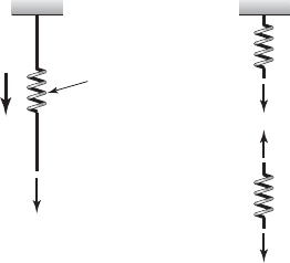
represents the internal force acting within the stiffness element, as
shown in the free-body diagram in Figure 2.5b, then in the lower spring por-
tion this force is equal and opposite to the external force F; that is,
Since the force F
s
tries to restore the stiffness element to its undeformed
configuration, it is referred to as a restoring force. As the stiffness element is
deformed, energy is stored in this element, and as the stiffness element is un-
deformed, energy is released. The potential energy V is defined
2
as the work
done to take the stiffness element from the deformed position to the un-
deformed position; that is, the work needed to undeform the element to its
original shape. For the element shown in Figure 2.5, this is given by
(2.8)
where we have used the identity j j 1 and F
s
Fj. Like the kinetic en-
ergy T, the potential energy V is a scalar-valued function.
The relationship between the deformation experienced by a spring and an
externally applied force may be linear as discussed in Section 2.3.2 or non-
0
x
Fj
#
dxj
x
0
Fdx
V1x 2
0
x
F
s
#
dx
F
s
Fj
30 CHAPTER 2 Modeling of Vibratory Systems
2
A general definition of potential energy V takes the form
where the force F
s
is a conservative force. The work done by a conservative force is independent
of the path followed between the initial and final positions.
V1x 2
initial or reference position
deformed position
F
s
#
dx
Stiffness
element
(b)(a)
j
F
s
F
F
FIGURE 2.5
(a) Stiffness element with a force
acting on it and (b) its free-body
diagram.
linear as discussed in Section 2.3.3. The notion of an equivalent spring ele-
ment is also introduced in Section 2.3.2.
2.3.2 Linear Springs
Translation Spring
If a force F is applied to a linear spring as shown in Figure 2.6a, this force pro-
duces a deflection x such that
(2.9)
where the coefficient k is called the spring constant and there is a linear rela-
tionship between the force and the displacement. Based on Eqs. (2.8) and
(2.9), the potential energy V stored in the spring is given by
(2.10)
Hence, for a linear spring, the associated potential energy is linearly propor-
tional to the spring stiffness k and proportional to the second power of the dis-
placement magnitude.
Torsion Spring
If a linear torsion spring is considered and if a moment t is applied to the
spring at one end while the other end of the spring is held fixed, then
(2.11)
where k
t
is the spring constant and u is the deformation of the spring. The po-
tential energy stored in this spring is
t1u 2 k
t
u
V1x 2
x
0
F1x 2dx
x
0
kxdx k
x
0
xdx
1
2
kx
2
F1x 2 kx
2.3 Stiffness Elements 31
x
(c)
k
1
k
2
F
k
(b)(a)
k
2
F
x
k
1
F
x
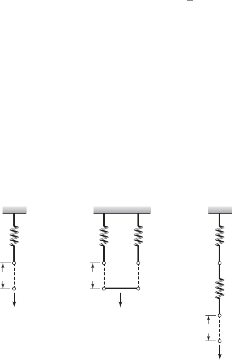
FIGURE 2.6
Various spring configurations:
(a) single spring, (b) two springs
in parallel, and (c) two springs in
series.
(2.12)
Combinations of Linear Springs
Different combinations of linear spring elements are now considered and the
equivalent stiffness of these combinations is determined. First, combinations
of translation springs shown in Figures 2.6b and 2.6c are considered and fol-
lowing that, combinations of torsion springs shown in Figures 2.7a and 2.7b
are considered.
When there are two springs in parallel as shown in Figure 2.6b and the
bar on which the force F acts remains parallel to its original position, then the
displacements of both springs are equal and, therefore, the total force is
(2.13)
where F
j
(x) is the resulting force in spring k
j
, j 1, 2, and k
e
is the equivalent
spring constant for two springs in parallel given by
(2.14)
When there are two springs in series, as shown in Figure 2.6c, the force
on each spring is the same and the total displacement is
(2.15)
where the equivalent spring constant k
e
is
(2.16)k
e
a
1
k
1
1
k
2
b
1
k
1
k
2
k
1
k
2
F
k
1
F
k
2
a
1
k
1
1
k
2
bF
F
k
e
x x
1
x
2
k
e
k
1
k
2
k
1
x k
2
x 1k
1
k
2
2x k
e
x
F1x 2 F
1
1x 2 F
2
1x 2
V1u 2
u
0
t1u 2du
u
0
k
t
udu
1
2
k
t
u
2
32 CHAPTER 2 Modeling of Vibratory Systems
(a)
k
t1
k
t2
(b)
k
t1
k
t2
FIGURE 2.7
Two torsion springs: (a) parallel combination and (b) series combination.

In general, for N springs in parallel, we have
(2.17)
and for N springs in series, we have
(2.18)
The potential energy for the spring combination shown in Figure 2.6b is
given by
where V
1
(x) is the potential energy associated with the spring of stiffness k
1
and V
2
(x) is the potential energy associated with the spring of stiffness k
2
.
Making use of Eq. (2.10) to determine V
1
(x) and V
2
(x), we find that
For the spring combination shown in Figure 2.6c, the potential energy of this
system is given by
where again Eq. (2.10) has been used. Expressions constructed from the po-
tential energy of systems are useful for determining the equations of motion
of a system, as discussed in Sections 3.6 and 7.2.
For two torsion springs in series and parallel combinations, we refer to
Figure 2.7. From Figure 2.7a, the rotation u of each spring is the same and,
therefore,
(2.19)
where t
j
is the resulting moment in spring k
tj
, j 1,2, and k
te
is the equivalent
torsional stiffness given by
(2.20)
For torsion springs in series, as shown in Figure 2.7b, the torque on each
spring is the same, but the rotations are unequal. Thus,
(2.21)u u
1
u
2
t
k
t1
t
k
t2
a
1
k
t1
1
k
t2
bt
t
k
te
k
te
k
t1
k
t2
k
t1
u k
t 2
u 1k
t1
k
t 2
2u k
te
u
t1u 2 t
1
1u 2 t
2
1u 2
1
2
k
1
x
1
2
1
2
k
2
x
2
2
V1x
1
, x
2
2 V
1
1x
1
2 V
2
1x
2
2
V1x 2
1
2
k
1
x
2
1
2
k
2
x
2
1
2
1k
1
k
2
2x
2
V1x 2 V
1
1x 2 V
2
1x 2
k
e
c
a
N
i 1
1
k
i
d
1
k
e
a
N
i 1
k
i
2.3 Stiffness Elements 33
where the equivalent stiffness k
te
is
(2.22)
The potential energy for the torsion-spring combination shown in Fig-
ure 2.7a is given by
where we have used Eq. (2.12). For the torsion-spring combination shown in
Figure 2.7b, the system potential energy is given by
Equivalent Spring Constants of Common Structural Elements
Used in Vibration Models
To determine the spring constant for numerous elastic structural elements one
can make use of known relationships between force and displacement.
Several such spring constants that have been determined for different geom-
etry and loading conditions are presented in Table 2.3. For modeling pur-
poses, the inertias of the structural elements such as the beams of Cases 4
to 6 in Table 2.3 are usually ignored. In Chapter 9, it is shown under what
conditions it is reasonable to make such an assumption.
3
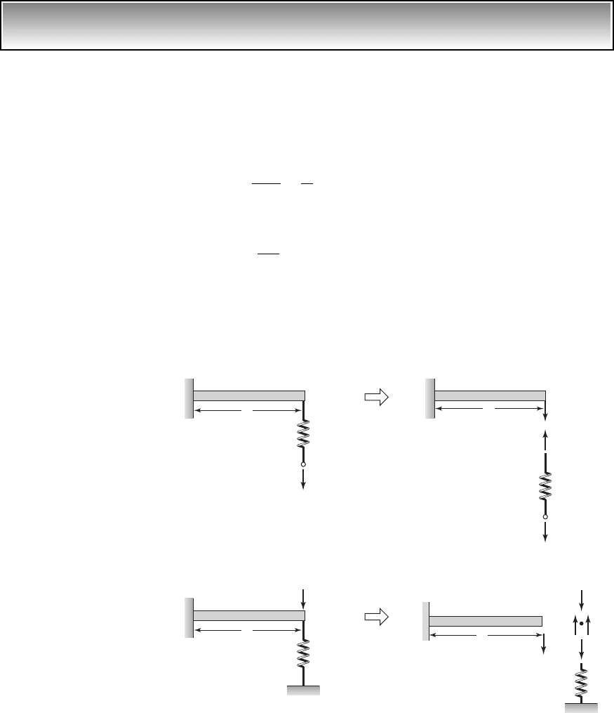
Since it may not always be possible to obtain a spring constant for a given
system through analysis, often one has to experimentally determine this con-
stant. As a representative example, let us return to Figure 2.4a, and consider
the experimental determination of the spring constant for this system. The
loading F is gradually increased to a chosen value and the resulting deflection
x from the unstretched position of the element is recorded for each value of F.
These data are plotted in Figure 2.8, where open squares are used to denote
the values of the experimentally obtained data. Then, assuming that the stiff-
ness element is linear, curve fitting is done to estimate the unknown param-
eter k in Eq. (2.9). The resulting value of the spring constant is also shown in
Figure 2.8. Note that the stiffness constant k is a static concept, and hence, a
static loading is sufficient to determine this parameter.
Force-displacement relationships other than Eq. (2.9) may also be used
to determine parameters such as k that characterize a stiffness element.
Determinationofparameters for anonlinearspring is discussedinSection 2.3.3.
In a broader context, procedures used to determine parameters such as k of a
vibratory system element fall under the area called system identification or
1
2
k
t
1
u
1
2
1
2
k
t
2
u
2
2
V1u
1
, u
2
2 V
1
1u
1
2 V
2
1u
2
2
1
2
k
t
1
u
2
1
2
k
t
2
u
2
1
2
1k
t
1
k
t
2
2u
2
V1u 2 V
1
1u 2 V
2
1u 2
k
te
a
1
k
t1
1
k
t 2
b
1
k
t1
k
t2
k
t1
k
t2
34 CHAPTER 2 Modeling of Vibratory Systems
3
See Eqs. (9.105) and (9.162).
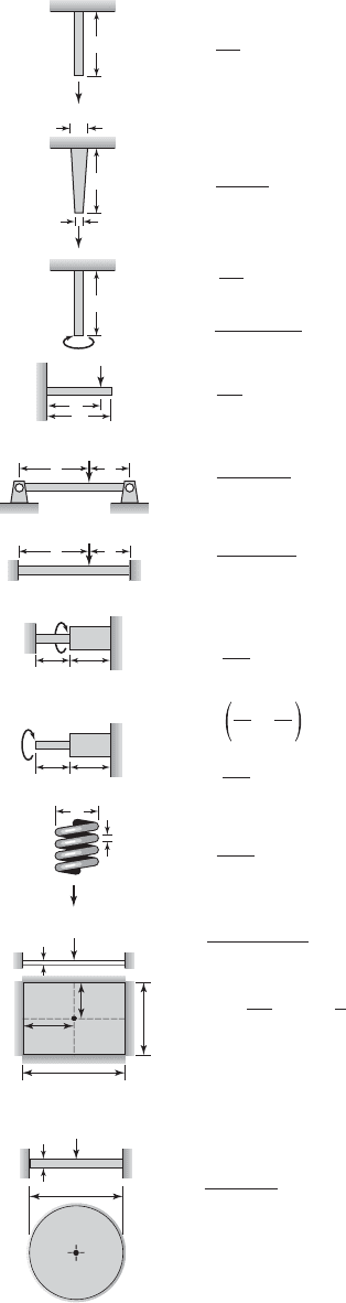
TABLE 2.3
Spring Constants for Some
Common Elastic Elements
F, x
L
,
,
,
L
F, x
F, x
F, x
b
a
a
L
L
d
1
d
2
L
1
L
2
F, x
F, x
n turns
D
d
b
a
k
t2
k
t1
L
1
L
2
k
t2
k
t1
1 Axially loaded rod or cable
k
k
AE
L
2 Axially loaded tapered rod
3 Hollow circular rod in torsion
32
4 Cantilever beam
5 Pinned-pinned beam
(Hinged, simply supported)
6 Clamped-clamped beam
(Fixed-fixed beam)
7 Two circular rods in torsion
8 Two circular rods in torsion
9 Coil spring
k
t
GI
L
k
t
i
G
i
I
i
L
i
k
t
i
G
i
I
i
L
i
k
Gd
4
8nD
3
Ed
1
d
2
4L
I
(d
out
d
in
)
44
3EI
k
k
k
; 0 a L
a
3
3EI(a b)
a
2
b
2
3EI(a b)
3
k
te
k
t1
k
t2
k
te
1
k
t1
1
k
t2
a
3
b
3
1
10
Clamped rectangular
plate, constant thickness,
force at center
a
b/a
α
1.0 0.00560
1.2 0.00647
1.4 0.00691
1.6 0.00712
1.8 0.00720
2.0 0.00722
11
Clamped circular plate,
constant thickness, force
at center
b
;
12
α
a
2
A1 v
2
B
Eh
3
v
Poisson's ratio
a
2
A1 v
2
B
4.189Eh
3
;
v
Poisson's ratio
k
k
b
/2
b
a
/2
a
F
h
2
a
h
F
(continued)
parameter identification; identification and estimation of parameters of
vibratory systems are addressed in the field of experimental modal analysis.
4
In experimental modal analysis, dynamic loading is used for parameter
estimation. A further discussion is provided in Chapter 5, when system input-
output relations (transfer functions and frequency response functions) are
considered.
Next, some examples are considered to illustrate how the information
shown in Table 2.3 can be used to determine equivalent spring constants for
different physical configurations.
36 CHAPTER 2 Modeling of Vibratory Systems
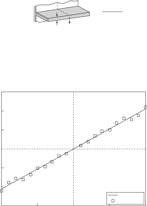
12
Cantilever plate, constant
thickness, force at center
of free edge
c
b
2
A1 v
2
B
0.496Eh
3
;
v
Poisson's ratio,
a
b
k
a
/2
a
/2
b
h
F
A: area of cross section; E: Young’s modulus; G: shear modulus; I: area moment of inertia or polar
moment of inertia
a
S. Timoshenko and S. Woinowsky-Krieger, Theory of Plates and Shells, McGraw-Hill, New York, (1959)
p. 206.
b
S. Timoshenko and S. Woinowsky-Krieger, ibid, p. 69.
c
S. Timoshenko and S. Woinowsky-Krieger, ibid, p. 210.
TABLE 2.3
(continued)
4
D. J. Ewins, Modal Testing: Theory and Practice, John Wiley and Sons, NY (1984).
1500
1000
k 10568 N/m
F (N)
500
0
500
1000
1500
0.1 0.05
0
x (m)
0.05 0.1
Fitted curve
Data
FIGURE 2.8
Experimentally obtained data used to determine the linear spring constant k.
EXAMPLE 2.3 Equivalent stiffness of a beam-spring combination
Consider the combinations shown in Figure 2.9. In Figures 2.9a and 2.9b, we
have a cantilever beam that has a spring attached at its free end. In Figure 2.9a,
the force is applied to the free end of the spring. In this case, the forces acting
on the cantilever beam and the spring are the same as seen from the associ-
ated free-body diagram, and, hence, the springs are in series. Thus, from
Eq. (2.18), we arrive at
(a)
where, from Table 2.3,
(b)
In Figure 2.9b, the force is applied simultaneously to the free end of
the cantilever beam and a linear spring of stiffness k
1
. In this case, the
k
beam
3EI
L
3
k
e
a
1
k
beam
1
k
1
b
1
2.3 Stiffness Elements 37
k
1
L
k
beam
(a)
(b)
F
F
1
F
2
F
2
F
1
F
k
1
L
k
beam
F
F
F
k
1
L
k
beam
F
L
k
1
k
beam
FIGURE 2.9
Spring combinations and free-body diagrams.
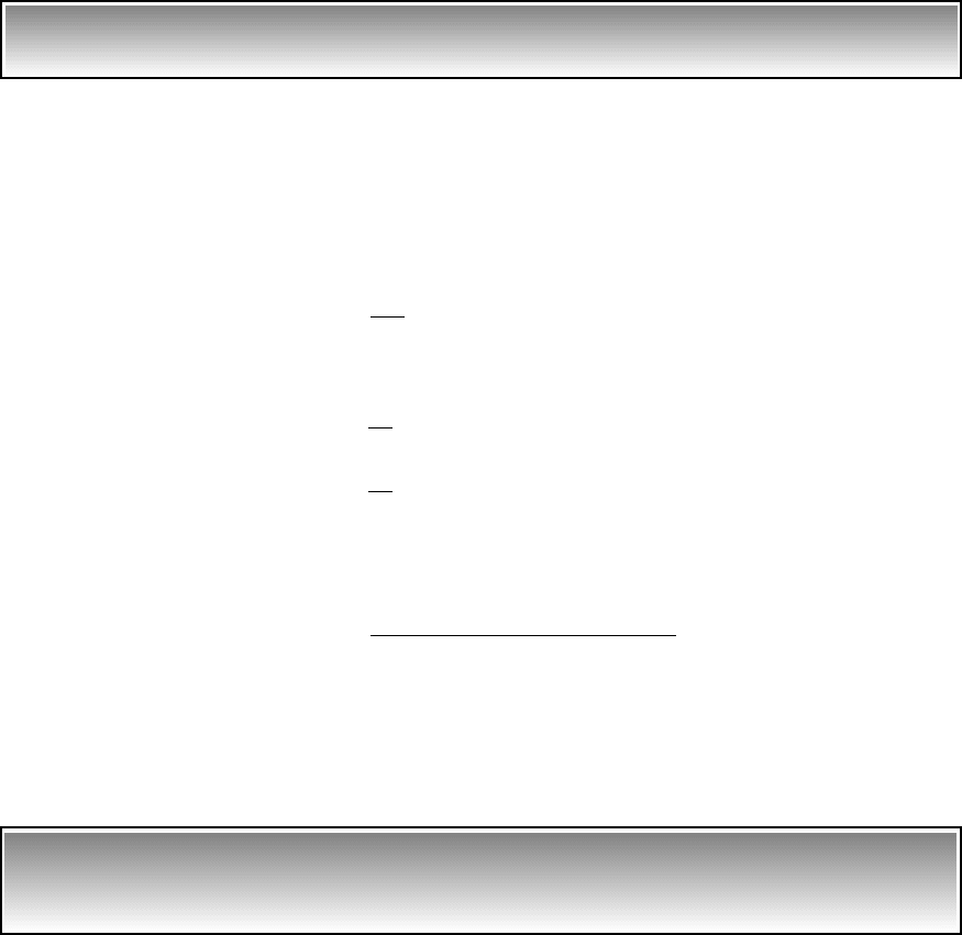
displacements at the attachment point of the cantilever and the spring are
equal and the springs are in parallel. Thus, from Eq. (2.17), we find that
(c)
EXAMPLE 2.4
Equivalent stiffness of a cantilever beam with a transverse end load
A cantilever beam, which is made of an alloy with the Young’s modulus of
elasticity E 72 10
9
N/m
2
, is loaded transversely at its free end. If the
length of the beam is 750 mm and the beam has an annular cross-section with
inner and outer diameters of 110 mm and 120 mm, respectively, then deter-
mine the equivalent stiffness of this beam.
For the given loading, the equivalent stiffness of the cantilever beam is
found from Case 4 of Table 2.3 to be
(a)
where the area moment of inertia I about the bending axis is determined as
(b)
Then, from Eq. (a)
N/m
N/m (c)
When the length is increased from 750 mm to twice its value—that is, to
1500 mm—the stiffness decreases by eightfold from 3.06 10
6
N/m to
0.383 10
6
N/m.
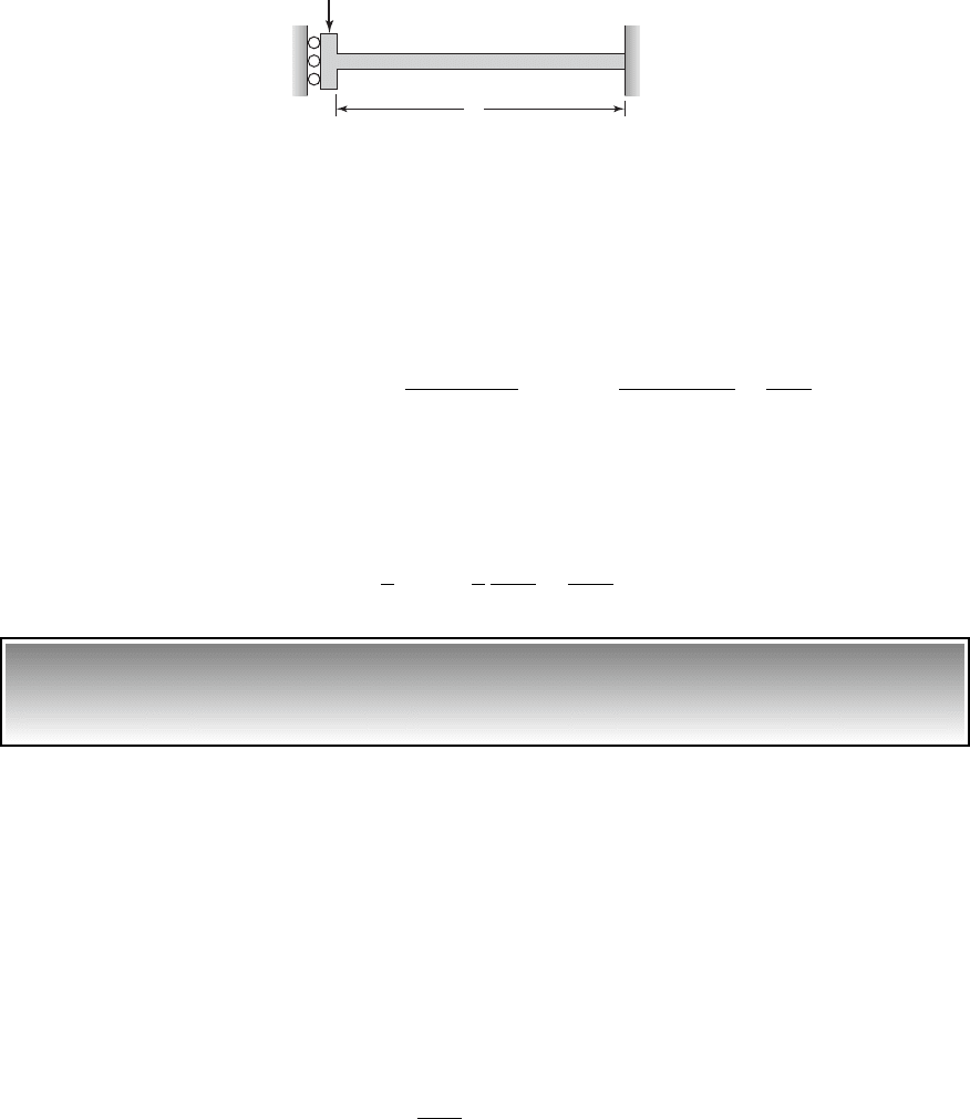
EXAMPLE 2.5
Equivalent stiffness of a beam with a fixed end and a translating
support at the other end
In Figure 2.10, a uniform beam of length L and flexural rigidity EI, where E is
the Young’s modulus of elasticity and I is the area moment of inertia about the
bending axis, is shown. This beam is fixed at one end and free to translate along
the vertical direction at the other end with the restraint that the beam slope is
zero at this end. The equivalent stiffness of this beam is to be determined when
the beam is subjected to a transverse loading F at the translating support end.
3.06 10
6
k
3 172 10
9
2 15.98 10
6
2
1750 10
3
2
3
5.98 10
6
m
4
p
32
31120 10
3
2
4
1110 10
3
2
4
4
I
p
32
1d
outer
4
d
inner
4
2
k
3EI
L
3
k
e
k
beam
k
1
38 CHAPTER 2 Modeling of Vibratory Systems
2.3 Stiffness Elements 39
Since the midpoint of a fixed-fixed beam with a transverse load at its mid-
dle behaves like a beam with a translating support end, we first determine the
equivalent stiffness of a fixed-fixed beam of length 2L that is loaded at its mid-
dle. To this end, we use Case 6 of Table 2.3 and set a b L and obtain
(a)
Recognizing that the equivalent stiffness of a fixed-fixed beam of length
2L loaded at its middle is equal to the total equivalent stiffness of a parallel-
spring combination of two end loaded beams of the form shown in Figure 2.10,
we obtain from Eq. (2.17) and Eq. (a) that
(b)
EXAMPLE 2.6
Equivalent stiffness of a microelectromechanical system (MEMS)
fixed-fixed flexure
5
A microelectromechanical sensor system (MEMS) consisting of four flexures is
shown in Figure 2.11. Each of these flexures is fixed at one end and connected
to a mass at the other end. The length of each flexure is L, the thickness of each
flexure is h, and the width of each flexure is b. A transverse loading acts on the
mass along the Z-direction, which is normal to the X-Y plane. Each flexure is fab-
ricated from a polysilicon material, which has a Young’s modulus of elasticity
E 150 GPa. If the length of each flexure is 100 m and the width and thick-
ness are each 2 m, then determine the equivalent stiffness of the system.
Each of the four flexures can be treated as a beam that is fixed at one end
and free to translate only at the other end, similar to the system shown in Fig-
ure 2.10. This means that the equivalent stiffness of each flexure is given by
Eq. (b) of Example 2.5 as
(a)k
flexure
12EI
L
3
k
e
1
2
k
fixed
1
2
24EI
L
3
12EI
L
3
k
fixed
3EI1a b 2
3
a
3
b
3
`
a b L
3EI1L L 2
3
L
3
L
3
24EI
L
3
F
L
FIGURE 2.10
Beam fixed at one end and free to translate at the other end.
5
G. K. Fedder, “Simulation of Microelectromechanical Systems,” Ph.D. dissertation, Department
of Electrical Engineering and Computer Sciences, University of California, Berkeley, CA (1994).