Awange J.,Grafarend E., Palancz B., Zaletnyik P. Algebraic Geodesy and Geoinformatics

Подождите немного. Документ загружается.

6-4 Solving nonlinear equations via homotopy 75

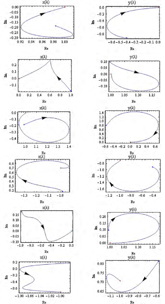
Figure 6.8. Homotopy paths starting from the six starting values expressed by (6.43)-

(6.48)

76 6 Linear homotpy

Table 6.4. Homotopy solutions of the system de scribed by Eqs. (6.31)-(6.32)

x y

0. 1.

1. 0.

−1. −0.707107i −1. + 0.707107i

−1. + 0.707107i −1. − 0.707107i

Computations can be easily achieved using the CAS system Mathematica, as illus-

trated in the Appendix A-3 where this example is solved.

Some features of our Mathematica implementation are as follows:

1. Direct computation of the homotopy paths using the standard Ne wton-

Raphson method.

2. Computation of the homotopy paths using numerical integration. An implicit

diﬀerential equation system can be transformed into an explicit one by com-

puter algebra for the case of 6-8 variables, or special numerical techniques

without inversion can be used for the case of higher dimensions.

3. Computation of a proper start system using Bezout’s theorem for systems

of multivariate polynomial equations, providing initial values for all paths of

roots.

4. Visualization of the paths of all trajectories for the case of arbitrary numbers

of variables and systems.

Generally, all of these functions can be parameterized freely, that is the start

system and the type of linear homotopy can be deﬁned by the user. In addition,

any computation can be carried out to any degree of precision.

6-5 Concluding remarks

As demonstrated in these examples, the linear homotopy method proves to be a

powerful solution tool in solving nonlinear geodetic problems, especially if it is

diﬃcult to ﬁnd proper initial values to ensure the convergence of local solution

methods. Linear homotopy is robust and enlarges the convergency region of the

local methods. This global numerical method c an be successful when symbolic

computation based on Groebner basis or Dixon resultant fail because of the size

and complexity of the problem. However, to reduce the number of paths to be

traced as indicated by Bezout’s theorem as the upper bound of the number of

solutions, it is important to ﬁnd a proper starting system to ensure fewer initial

value problems to solve.

This method provides the geodesy community with an additional powerful

mathematical tool that is useful, not only in root ﬁnding, but also in solving

6-5 Concluding remarks 77

complex problems that can be transformed into systems of p olynomial equations.

We have also shown that it oﬀers faster computations and in some cases solves

complex problems where existing methods such as Groebner basis or eve n local

numerical methods, such as Newton-type methods, fail.

7 Solutions of Overdetermined Systems

“Pauca des Matura” –a few but ripe – C. F. Gauss

7-1 Estimating geodetic and geoinformatics unknowns

In geodesy and geoinformatics, ﬁeld observations are normally collected with the

aim of estimating parameters. Very frequently, one has to handle overdetermined

systems of nonlinear equations. In such cases, there exist more equations than

unknowns, therefore “the solution” of the system can be interpreted only in least

squares sense.

In geodynamics for example, GPS and gravity measurements are undertaken

with the aim of determining crustal deformation. With improvement in instrumen-

tation, more observations are often collected than the unknowns. Let us consider a

simple case of measuring structural deformation. For deformable surfaces, such as

mining areas, or structures (e.g., bridges), several observable points are normally

marked on the surface of the body. These points would then be observed from a

network of points set up on a non-deformable stable surface. Measurements taken

are distances, angles or directions which are normally more than the unknown

positions of the points marked on the deformable surface leading to redundant

observations.

Procedures that are often used to estimate the unknowns from the measured

values will depend on the nature of the equations relating the observations to the

unknowns. If these equations are linear, then the task is much simpler. In such

cases, any procedure that can invert the normal equation matrix such as least

squares, linear Gauss-Markov model etc., would suﬃce. Least squares problems can

be linear or nonlinear. The linear least squares problem has a closed form (exact)

solution while the nonlinear problem does not. They ﬁrst have to be linearized

and the unknown parameters estimated by iterative reﬁnements; at each iteration

the system is approximated by a linear one.

Procedures for estimating parameters in linear models have bee n documented

in [244]. Press et al. [334] present algorithms for solving linear systems of equa-

tions. If the equations relating the observations to the unknowns are nonlinear

as already stated, they have ﬁrst to be linearized and the unknown parameters

estimated iteratively using numerical methods. The operations of these numer-

ical methods require some approximate starting values. At each iteration step,

the preceding estimated values of the unknowns are improved. The iteration steps

are repeated until the diﬀerence between two consecutive estimates of the un-

knowns satisﬁes a speciﬁed threshold. Procedures for solving nonlinear problems

such as the Steepest-descent, Newton’s, Newton-Rapson and Gauss-Newton’s have

been discussed in [334, 379]. In particular, [379] recommends the Gauss-Newton’s

method as it exploits the structure of the objective function (sum of squares)

that is to be minimized. In [381], the manifestation of the nonlinearity of a

function during the various stages of adjustment is considered. While extending

J.L. Awange et al., Algebraic Geodesy and Geoinformatics, 2nd ed.,

DOI 10.1007/978-3-642-12124-1 7,

 Springer-Verlag Berlin Heidelberg 2010

80 7 Solutions of O verdetermined Systems

the work of [252] on nonlinear adjustment with respect to geometric interpreta-

tion, [178, 179] have presented the necessary and suﬃcient conditions for least

squares adjustment of nonlinear Gauss-Markov model, and provided the geomet-

rical interpretation of these conditions. Another geometrical approach include the

work of [83], while non geometrically treatment of nonlinear problems have been

presented by [61, 255, 297, 332, 350, 354].

This Chapter presents diﬀerent approaches for solving the problem. Two pro-

cedures; the Algebraic LEast Square Solution (ALESS) discussed in Sect. 7-2 and

the Gauss- Jacobi combinatorial approach presented in Sect. 7-3. For the ALESS

approach, the original problem is transformed into a minimization problem con-

structing the objective function symbolically. The overdetermined system is then

converted into a determined one by deﬁning the objective function as the sum of

the square of residuals of the equations. The necessary condition for the mini-

mum is set such that each partial derivatives of the objective function should be

zero. In this case the determined model will consist of as many equations as many

parameters that were in the original overdetermined model.

7-2 Algebraic LEast Square Solution (ALESS)

7-21 Transforming overdetermined systems to determined

Let ∆ be the objective function to be minimized

∆(p

, p

, ..., p

) =

, (7.1)

where n is the number of the unknown parameters - p

(j = 1 . . . n) - and

(i = 1 . . . m) are the observational equations. The objective function should

be minimized according to the necessary condition of the minimum,

∂∆

∂p

= 0,

∂∆

∂p

= 0, . . . ,

∂∆

∂p

= 0. (7.2)

Now the system consists of as many equations as the number of the unknown

parameters. The solution of the original, overdetermined system (in least square

sense) will also be the solution of this “square determined system”.

Let us suppose, that our nonlinear system is a system of multivariate polyno-

mial equations, then the following theorem can be considered:

Theorem 7.1. Given m algebraic (polynomial) observational equations, where m

is the dimension of the observation space Y of order l in n unknown variables, and

n is the dimension of the parameter space X. Then there exists n normal equations

of the polynomial order (2l − 1) to be solved with algebraic methods.

This solution will be the algebraic least square solution (ALESS) of the overdeter-

mined system.

7-2 Algebraic LEast Square Solution (ALESS) 81

Proof

Let us consider the following s ystem,

(x, y) = x

+ y − 3

(x, y) = x +

− 1

(x, y) = x − y

here n = 2, m = 3 and l = 2. The objective function to be minimized is

∆ = e

+ e

= 10 − 2x − 4x

+ x

− 6y − 2xy + 2x

y +

The order of the objective function is 2l = 4. The overdetermined system has

one solution from the point of view of least square sense, the minimum of this

objective function.

Now, We need to ﬁnd the solutions of the original system by solving the deter-

mined problem. Considering the necessary condition for the minimum as

∂∆

∂x

= −2 − 8x + 4x

− 2y + 4xy +

= 0

∂∆

∂y

= −6 − 2x + 2x

y +

xy +

= 0,

one obtains the determined system whose order is 2l − 1 = 3. Solving this square

system leads to 6 complex solutions and 3 real ones. The real solutions are

= −1.371 y

= −0.177989

= 1.24747 y

= 1.27393

= −2.69566 y

= −4.24638,

which upon being substituted to the objective function ∆ results into the residuals

) as

= 8.71186

= 0.232361

= 4.48362.

From these residuals, the admissible real solutions is the one which provides the

least value of the residual (r

), i.e., the second solution. I n this case, the solution

in least squares sense is

= 1.24747 y

= 1.27393.

♣

82 7 Solutions of O verdetermined Systems

7-22 Solving the determined system

It is possible to ﬁnd the solutions of the determined square system using local or

global methods. Local methods such as the extended Newton-Raphson (see Chap.

9) or homotopy (see Chap. 7)) can be used if a good initial values are known.

Usually, these initial values can be calculated from the solution of a minimal subset

(see Palancz et al [322, 323, 430]). Using global methods, one should ﬁnd all of the

real solutions of the determined system representing the original overdetermined

system. This is then followed by selecting solutions that provide the least value of

the objective function.

Let us examine two methods of ﬁnding all of the roots of the previous polyno-

mial system. The two main types of the algebraic methods that are at our disposal,

which we have encountered in the previous chapters are:

• symbolic solutions using computer algebra as resultants or Groebner basis

• global numerical methods like linear homotopy

As an illustration, considering our problem, we solve the polynomial system via

reduced Groebner basis using M athematica as

GroebnerBasis[{f

, f

}, {x, y}, {y}]

GroebnerBasis[{f

, f

}, {x, y}, {x}],

which leads to

− 318 + 256x −231x

− 292x

+ 166x

+ 186x

+ 44x

− 56x

+ 8x

= 0,

− 24576 − 110592y + 147456y

− 39168y

+ 2016y

− 48y

+ 104y

+ y

= 0.

Solving the above univariate polynomials provide the real solution for variable x

= −2.69566 x

= −1.371 x

= 1.24747,

and those of the variable y as

= −4.24638 y

= −0.177989 y

= 1.27393,

which are the same solutions we obtained in the previous section. The solutions

giving minimum residuals are

x = 1.24747 y = 1.27393.

In general, for exact solution of determined systems, NSolve, the built-in function

of Mathematica, which utilize numerical Groebner basis seems to be a good choice.

However, if the system has many roots without physical meaning and one does

not need to compute all of the roots, the linear homotopy of ﬁxed point or Find-

Root built-in Mathematica can be an appropriate method. Whereas the statement

above refers to Mathematica, it is essential for users to know that other algebraic

packages, e.g., Matlab and Maple also have similar capabilities as Mathematica.

7-2 Algebraic LEast Square Solution (ALESS) 83

To demonstrate the global numerical me thod, let us employ the linear homo-

topy. As our example is a polynomial system, we can use the automatically gen-

erated start systems with random complex numbers (see Sect. 6-423). The target

system is given by

(x, y) = −2 − 8x + 4x

− 2y + 4xy +

= 0

(x, y) = −6 − 2x + 2x

y +

xy +

= 0.

with x, y variables. The degrees of the polynomials are d

= 3 and d

= 3. The

start system is given by

(x, y) = (−0.814932 + 0.579556i)(−0.550639 + 0.834743i + x

)

(x, y) = (0.858366 − 0.513038i)(−0.77 − 0.638044i + y

)

and its initial values, the solutions of the start system are presented in Table 7.1.

Table 7.1. Initial values of the homotopy function

x y

−0.193155 + 0.981168i −0.288775 − 0.957397i

−0.193155 + 0.981168i 0.973518 + 0.228612i

−0.193155 + 0.981168i −0.684743 + 0.728785i

−0.753139 −0.657861i −0.288775 − 0.957397i

−0.753139 −0.657861i 0.973518 + 0.228612i

−0.753139 −0.657861i −0.684743 + 0.728785i

0.946294 −0.323307i −0.288775 −0.957397i

0.946294 −0.323307i 0.973518 + 0.228612i

0.946294 −0.323307i −0.684743 + 0.728785i

The number of paths is 9. Employing the direct path tracing technique we get

as solutions in Table 7.2.

Table 7.2. End points of the homotopy paths

x y

−1.371 −0.177989

−0.987112 + 1.25442i 2.21036 + 1.61614i

−2.69566 −4.24638

0.33941 + 0.679091i −0.606933 − 7.81887i

−0.987112 −1.25442i 2.21036 − 1.61614i

0.33941 −0.679091i −0.606933 + 7.81887i

2.0573 + 1.28006i −0.0282082 − 7.43985i

1.24747 1.27393

2.0573 −1.28006i −0.0282082 + 7.43985i

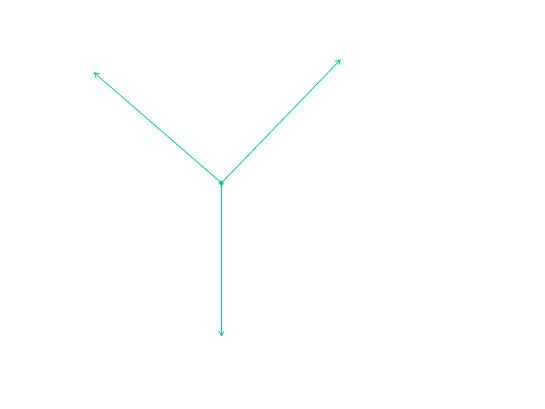
The real solutions are the same as we have seen before. The paths of the good

solution can be seen in Fig. 7.1.

84 7 Solutions of O verdetermined Systems

Figure 7.1. The paths of the good solution

7-3 Gauss-Jacobi combinatorial algorithm

In this section a combinatorial method is presented. The advantage of this method

is that solving a sub-problems in symbolic form, the numerical solution of all of the

combinatorial subproblems can be speedily computed, and using proper weight-

ing technique, the solutions can be e asily achieved. However, the disadvantage of

the method is that for a vastly overdetermined problem, combinatorial explosion

results. To avoid this, one of the appropriate approaches is to solve a few sub-

problems in a closed form and choose the initial solutions that are in the correct

vicinity of the desired solutions and use them as starting values for a least square

optimization. In Mathematica for example, choosing initial solutions that are in

the correct vicinity would involve calling FindMinimum, (Lichtblau, Private Com-

munication) and in Lichtblau[269]. Alternatively, another lo c al method, e.g., the

Extended Newton-Raphson method discussed in Chap. 8 can also be employed

starting with the weighted sub-problem solutions.

7-31 Combinatorial approach: the origin

Presented in this chapter is an alternative approach to traditional iterative numer-

ical procedures for solving overdetermined problems, i.e., where more observations

than unknown exist. This approach, which we call the Gauss-Jacobi combinatorial

has the following advantages:

1. From the start, the objective is known.

2. It does not require linearization.

3. The nee d for iteration does not exist.

4. The variance-covariance matrices of all parameters are considered.

5. It c an be exploited for outlier diagnosis.

The combinatorial approach traces its roots to the work of C. F. Gauss which

was published p osthumously (see Appendix A-2). Whereas the procedures pre-

sented in Chaps. 4 and 5 solve nonlinear systems of equations where the number

of observations n and unknowns m are equal, i.e., n = m, Gauss-Jacobi combina-

torial solves the case where n > m. In Fig. 4.1 on p. 34 for example, two distance

7-3 Gauss-Jacobi combinatorial algorithm 85

measurements from known stations P

and P

were used to determine the position

of unknown station P

. Let us assume that instead of the two known stations,

a third distance was measured from p oint P

as depicted in Fig. 7.2. In such a

Figure 7.2. Planar distance observations

case, there exist three possibilities (combinations) for determining the position of

the unknown station P

. Recall that for Fig. 4.1 on p. 34, two nonlinear distance

equations were written (e.g., 4.1 and 4.2). For Fig. 7.2, systems of distance equa-

tions could be written for combinations {P

}, {P

} and {P

}. For

combination {P

} for example, one writes

= (x

− x

)

+ (y

− y

)

(7.3)

and

= (x

− x

)

+ (y

− y

)

. (7.4)

Equations (7.3) and (7.4) lead to solutions {x

, y

}

1,2

as position of the unknown

station P

, where the subscripts indicate the combinations used. Combination

} gives

= (x

− x

)

+ (y

− y

)

(7.5)

and

= (x

− x

)

+ (y

− y

)

, (7.6)

leading to solutions {x

, y

}

1,3

as the position of the unknown station P

. The last

combination {P

} has

= (x

− x

)

+ (y

− y

)

(7.7)

and