Angermann L. (ed.). Numerical Simulations - Applications, Examples and Theory

Подождите немного. Документ загружается.

Hybrid Type Method of Numerical Solution Integral Equations and its Applications

491

Having generated the points with the density p

opt

(y), received from (5) by approximated

values φ

, we can get a more precise solution of the equation (1). After that with this

equation and by means of (5) we can calculate again (more precise) value of optimal density.

The process can be repeated till the density stops changing. This is the main sense of

adaptive algorithm of choosing an optimal density.

3. Statement of the problem of blade cascade flow

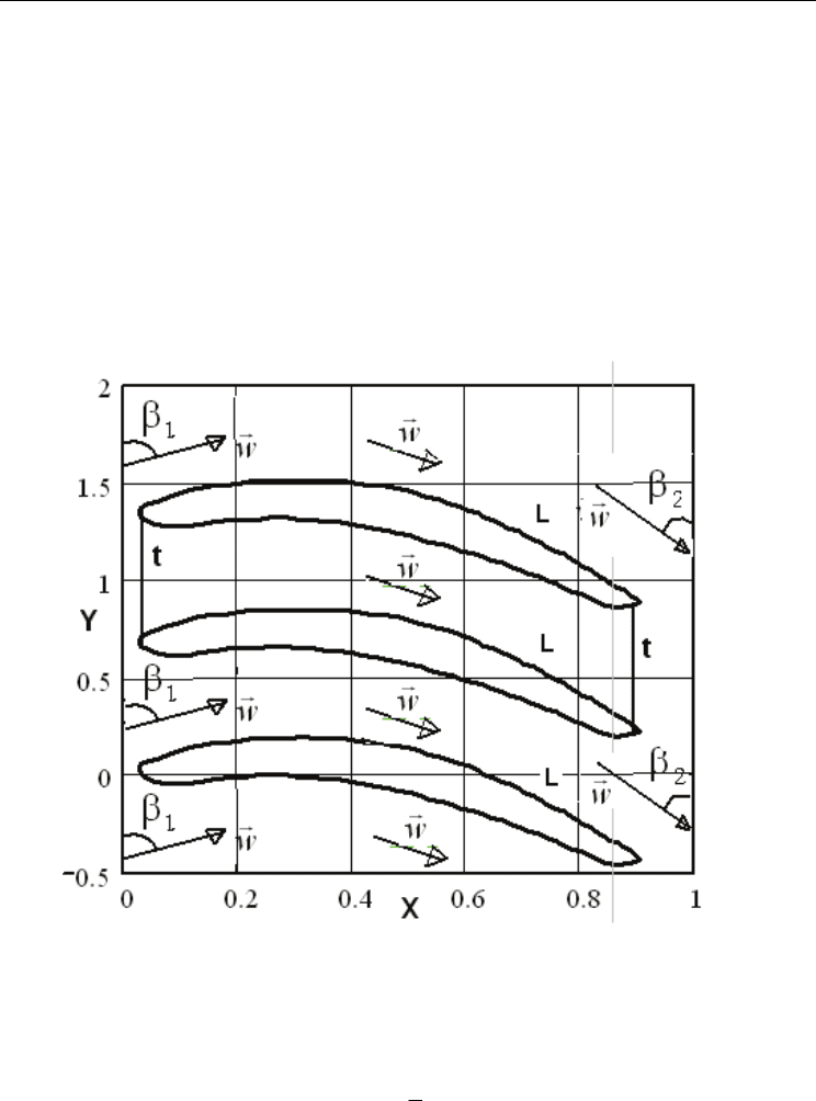
A plane lattice with the increment t (Fig. 1) is given, on which from the infinity under the

angle β

a potential flow of ideal fluid is leaking, coming out from a lattice under the angle

. The task is to find an absolute value of a normed speed of the flow on the edging of the

profiles.

Fig. 1. Lattice of the profiles. w

is a vector of the flow speed, t is an increment of the lattice,

is and input angle of the flow, β

is and output angle of the flow, L is a contour of the

blade profile

This task comes [5] to the solution of integral equation of the following kind:

() () ()

ws K sl w l dl b s

() ,

⎛⎞

+−⋅=

⎜⎟

⎝⎠

∫v

, (6)

where w(s)– normed speed of the flow;

Numerical Simulations - Applications, Examples and Theory

492

()

() ()

()

() ()

()

() ()

()

() ()

()

lxsxl

st s t

Ksl

ys yl xs xl

sin sinh

cos cosh

ππ

∂

⎛⎞⎛⎞

⋅⋅−− ⋅−

⎜⎟⎜⎟

∂∂

⎝⎠⎝⎠

=⋅

⎛⎞⎛⎞

⋅− − ⋅−

⎜⎟⎜⎟

⎝⎠⎝⎠

;

() ()

()

ss L

( ) 2 cot cot

ββ

∂

=− ⋅ − ⋅ + +

∂∂

Here s and l are values of the arch in different points of profile’s edges, arches are counted

from the middle of exiting border of the profile in the positive direction (counterclockwise);

x(l), y(l) are the coordinates of the profile’s point with the length of the arch l;

L is a contour

of the blade profile;

L is the length of the contour of the blade profile.

The direction of the unit tangent vector

∂

⎧

⎫

⎨

⎬

∂

⎩⎭

is chosen in a way that the tracking of the

contour would be made counterclockwise. As opposed to [5], in this research front side of

the lattice is orientated not along the abscises axis, but along the ordinate axis. Besides that,

in [5] the speed is normed so that the flow expense of the fluid on the output would be

unitary, and in this research the speed is normed so that the absolute value of speed vector

on the outcome of the lattice would be unitary. This is achieved by multiplication of the

speed, received after solving equations (1) and sin(β

). Exactly the second norm rate setting

is applied in the computational program of the Ural Polytechnic Institute (UPI), where the

computations were made with the method of rectangles with the optimal setting of the

integration nodes [2, 6] The solutions, received in this program, have been chosen for the

comparison in this research.

4. Scheme of application of semi-statical method to the problem of blade

cascade flow

4.1 Main formulas

In this task contour L acts as a surface S, and an integral equation (6) with an unknown

function w(s) is solved. If by w

(s) we define an average solution after k iterations, and by

(s) - value received on the integration with the number k after solving integral equation

(1) on the N number of generated points, then we’ll have

() ()

ws Ws

=⋅

∑

(7)

Selective standard deviation on the iteration with the number k is computated with the

formula:

() ()

sDs

=⋅

∑

, (8)

where D

–selective dispersion in the end of one iteration with the number l;

Hybrid Type Method of Numerical Solution Integral Equations and its Applications

493

()

( ) () ()

lkmk

Ksl

Ds Wl bs Ws

NN pl

⎛⎞

−

⎜⎟

=⋅+−

⎜⎟

−

⎜⎟

⎝⎠

∑

Here l

, l

, …,l

are random points on the segment [0, 2π], thrown on the iteration number

k, N- a number of points in each iteration (in given below computational calculations is

similar for all iterations), s-point of observation. Values of w(l

) are received as a result of

approximated solution of integral equation (1) at the interation number k- of the method.

Computational practice has shown that deviation (calculating error) do not go behind the

limits of standard deviation multiplied by three and, as usual, are within the boundaries of

standard confidential (95%) interval.

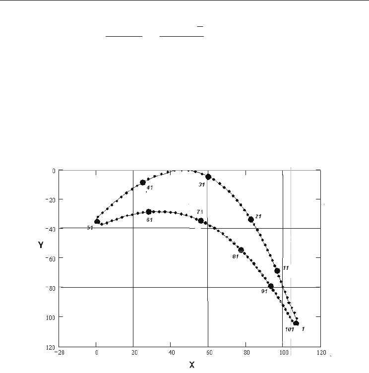
Fig. 2. Points, where the speed is calculated in computational examples – 50 equi-spaced

points on the back and on the trough

Analytic definition of the blade contour

Integral equation (6) on the smooth contour L is of fredgolm type and has a unique solution

[5]. Kernel of the equation (6) in case of two times differentiated contour can be considered

continuous, as it has a removable singularity when s=l [5]. In this research, however,

contour is defined by a spline curve, first derivative of which has jumps in the finite set of

points. This circumstance leads to the jumps of the kernel in the break points of the first

derivative, which doesn’t however influence the quality of computations. Besides that, the

spline can always be approximated by a segment of Fourier row and the task can be solved

on the infinitely derivated contour, as shown in [6].

Both approaches were tested, and the solutions made on a spline and on a segment of

Fourier row were not considerably different. Semi-statical method was applied to the

Numerical Simulations - Applications, Examples and Theory

494

equation (1) in accordance with the general scheme, which is described in detail in [3],

without any additional preparation of regularization type. Values of the speed were

calculated in 100 points of edging, 50 equal-spaced points on the trough and on the back

correspondingly (Fig. 2). After that they were multiplied by sin(β

), the result was compared

to the solution, received by means of method of rectangles at the same contour. Both results

were compared that to the one given by the UPI program. In the UPI program the contour is

defined a little bit different, which causes insignificant divergences, which can be seen of the

diagrams in the section of the results of computational modeling.

4.2 Computation algorithm and optimization.

The calculating was made iteratively. On each iteration a special number of random points

on the segment [0, 2π] was generated with the density, which was calculated by the results

of previous iterations (adaptive algorithm). On the first iterations points were generated

with uniform density on the segment [0, 2π], which means approximately uniform

distribution of the points on the contour of the blade, the results were defining more

precisely by iterations, and approximated solution after iteration number i was considered

to be arithmetic average of the solutions, received during previous iterations.

With the help of this approximated solution optimal density was calculated, using the

method, described in [1]. Here algorithm is more economical, than described in [1], as it uses

a more precise approximation to the right decision. As the computational practice has

proved, on the strongly stretched contours on some iterations very strong spikes are

possible, which are not smoothed by approximation even with the big number of iterations.

However, it turned out that if the solution is very imprecise, than selective dispersions are

also big in the check points, which are calculated during the work of the program.

We can introduce a constraint which will trace summands with a very big dispersion. In the

current research the program is composed in a way that approximation is made not on all

iterations, but only in those where relevant computational error, defined by the selective

dispersion, is not bigger that 100 percent. Other solutions received on other iterations

(usually not more than one percent from total number with the exclusion of the points close

to edgings), are considered as spikes and are not included into the approximated finite sum.

In case of much stretched working blade this improvement gives an undoubted advantage

in the quality of computations.

With the help of semi-statistical method values of the speed were calculated in 150 points,

distributed on the contour of the blade with an equal increment defined by the parameter u

(which means practically equal increment on the arch length), and the values of the speed in

checkpoints (which are distributed in the contour not evenly) were calculated with the help

of interpolation. Selective dispersion is used as an index of precision of current

approximation. It turned out that computer spends the most of time to calculating values of

the kernel in the generated points, that’s why the issue of decreasing number of generated

points but saving precision of computation at the same time is important. In semi-statistical

methods this can be achieved by optimization of the net of integration.

5. Results of computational modeling

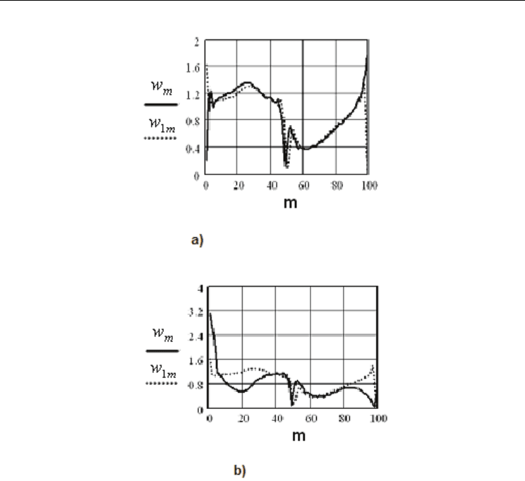
To continue, let us introduce some denominations. On all the figures from 3 to 5 variable m

stands for the number of point of observation, w

is the speed in the point number m,

Hybrid Type Method of Numerical Solution Integral Equations and its Applications

495

calculated by means of semi-statistical method, w

is the speed in point number m,

calculated by means of method of rectangles, w

is the speed in point number m, calculated

by means of UPI program, │w

−w

│is absolute deviation (calculation error) of calculation

of the speed in point number m by means of semi-statistical method in comparison to the

method of rectangles. Phrase “speed, calculated by means of semi-statistical method

(4*400)” will mean that for calculation 4 iterations of semi-statistical method were made,

with 400 points generated in every iteration.

Next (Fig. 3 – Fig. 5) the results of computational modeling are shown.

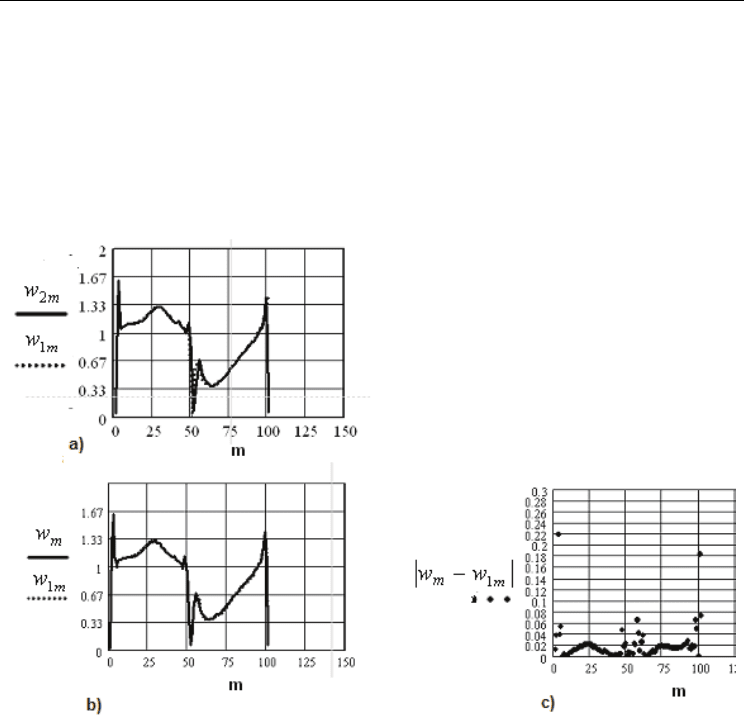
Fig. 3. Results of computational modeling on blade:

a) Speed graph, calculated by means of method of rectangles and speed graph

calculated by means of UPI program

b) Speed graph, calculated by means of semi-statistical method (150*400) and speed

graph, calculated by means of method of rectangles

c) Absolute deviation graph of calculation of the speed by means of semi- statistical

method (150*400) in comparison to the method of rectangles

From given above examples (Fig.3) it is evident, that semi-statistical method commutated

the speed with a good precision in all the points of contour, except for some points in the

edgings, which are not important for practical issues.

6. Analysis of effectiveness of density adaptation

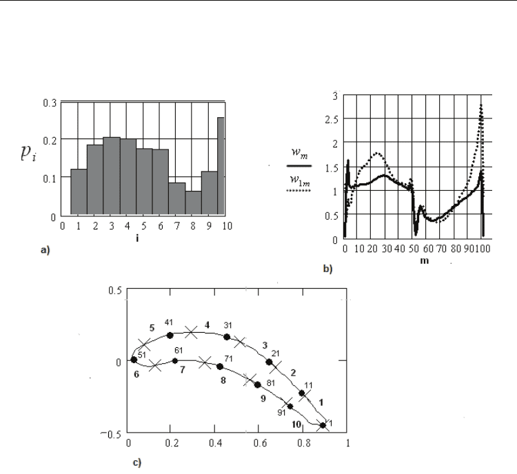
It was very interesting to investigate, how adaptive algorithm works when choosing optimal

density. It appears that the points become denser on the edgings and on the back, which

Numerical Simulations - Applications, Examples and Theory

496

means exactly the same places of profile, where the quality of computation is very bad

during first iterations.

This is illustrated by the Fig. 4.

Fig. 4.

a) Histogram of optimal density after 2 iterations on the blade;

b) Speed graph calculated of the speed by means of semi-statistical method (2

iterations 400 points each) and speed graph calculated by means of method of

rectangles.

c) With the symbol “

” borders of intervals from histogram on the Fig.3 a) are

marked; numbers 1,2,…10 are the numbers of these intervals. Bold points are

checkpoints (marked every 10 points starting with first); numbers 1,11,21,…92 –

numbers of these points

On the Fig. 5 the results of computations on blade are shown, received after five iterations

using adaptive algorithm for choice of optimal density and the results, received after five

iterations with even distribution of generated points. It is easy to see that with the same

number of generated points the results of adaptive algorithm are more precise.

From the Fig. 5 it is clear that using adaptive algorithm makes standard mean-square

distance lower in shorter period, that with even distribution. It allows reducing the number

of thrown points which is necessary to achieve predefined precision.

Hybrid Type Method of Numerical Solution Integral Equations and its Applications

497

Fig. 5. Results of computational modeling on blade:

a) Speed graph, calculated by means of semi-statical method (5*400) and speed graph,

with the use of adaptive algorithm, calculated by means of method of rectangles

b) Speed graph, calculated by means of semi-statical method (5*400) and speed graph,

without the use of adaptive algorithm, calculated by means of method of rectangles

7. Conclusions

To sum up the results of computational modeling, following conclusions can be drawn:

By means of semi-statical method quite precise results can be achieved solving the

problem of potential lattice cascade flow.

In accordance with theoretical computations adaptive algorithm works for optimization

of nodes on the domain of integration. It fastens convergence, reducing selective

dispersion.

However in strongly-stretched areas convergence rate is not very fast. The problem of

fastening the rate of convergence, which is necessary to make semi-statical method

successive in case of strongly-stretched areas and make it competitive to deterministic

Numerical Simulations - Applications, Examples and Theory

498

methods in calculation speed, is still important. One of the ways to solve this problem

is, evidently, improvement of the adaptive algorithm of optimization.

8. References

Arsenjev D.G., Ivanov V.M., Kul'chitsky O.Y. (1999). Adaptive methods of computing

mathematics and mechanics. Stochastic variant. World Scientific Publishing Co.,

Singapore

Arsenjev D.G., Ivanov V.M., Korenevsky M.L. (2004). Semi-statistical and projection-

statistical methods of numerical solving integral equations. World Scientific and

Engineering Academy and Society (WSEAS) Transactions on Circuits and Systems, Issue

9, Volume 3: 1745-1749

Arsenjev D.G., Ivanov V.M., Berkovskiy N.A. (2004). Application of semi-statical method to

inside Dirichle problem in three-dimensional space. Scientific proceedings of SPbSPU,

St.Petersburg, № 4 (38):52–59

Isakov S.N., Tugushev N.U., Pirogova I.N. (1984). Report on scientific research.

Development of computational software for calculating field of velocities and

profile losses in lattices in compression in turbine buckets. Proceedings of Ural

polytechnical institute, Svedrdlovsk

Jhukovskiy M.I. (1967). Aerodynamic computing of flow in axial turbo-machines. Mashgiz,

Leningrad

Vochmyanin S.M., Roost E.G., Bogov I.A. (1997). Computing cooling systems for gas turbine

blades. Bundled software GOLD. International academy of high school, Petersburg

Part 6

Safety Simulation