Amano R.S., Sunden B. (Eds.) Computational Fluid Dynamics and Heat Transfer: Emerging Topics
Подождите немного. Документ загружается.

Sunden CH012.tex 17/8/2010 20: 31 Page 466
466 Computational Fluid Dynamics and Heat Transfer
and if this expression is substituted in equation (13), we arrive to expression
Q
(ν)
= F(Q
(ν−1)
+Q
(ν−1)
) −F(Q
(ν−1)
) (15)
Using the linear expansion of the term F(Q
(ν−1)
+Q
(ν−1)
) in the previous
equation, we obtain
F(Q
(ν−1)
+Q
(ν−1)
) = F(Q
(ν−1)
) +∂
Q
F(Q
(ν−1)
) +O(ε
2
) (16)
Neglecting the terms of higher order, expression in equation (16) becomes
F(Q
(ν−1)
+Q
(ν−1)
) ≈ F(Q
(ν−1)
) +∂
Q
F(Q
(ν−1)
) (17)
Substituting equation (17) into equation (15), expression linking Q
(ν)
and
Q
(ν−1)
is formulated
Q
(ν)
≈ ∂
Q
F(Q
(ν−1)
)Q
(ν−1)
(18)
By letting the index ν to range from 0 to ν +1, equation (18) is used recursively to
obtain the link between Q
(0)
and Q
(ν+1)
Q
(ν+1)
≈ (∂
Q
F(Q
(ν)
))
ν
Q
(0)
(19)
The recursive property of the fixed-point algorithm is given by equation (19) and
uponcloserinspectionitcanbeseenthatitrepresents,apoweriterationofQ
(ν+1)
with matrix ∂
Q
F(Q
(ν)
), within second order of accuracy. Moreover, it can also be
observed that the sequence of Q
(ν+1)
vectors will tend to lie in the dominant
eigenspace of matrix ∂
Q
F(Q
(ν)
) and also define the basis of the Krylov subspace
associated with the iterative procedure described by the fixed-point method, equa-
tion(9).Thispropertyisusedtoapproximatethesolutionofthefixed-pointproblem
byusing the minimal polynomial of the Jacobian matrix ∂
Q
F(Q
(ν)
).A Krylov sub-
space generated by the iterative process defined by equation (10) can be defined
formally by using the local linearization of the fixed-point function
K
n
(M
−1
(∂
Q
R),R
(0)
) = span(R
(0)
,(M
−1
(∂
Q
R))R
(0)
,...,(M
−1
(∂
Q
R))
n−1
R
(0)
)
(20)
Since in equation (20) operator M is kept constant in the local neighborhood of
solution vectors, Krylov subspace K
n
can be shown to be equivalent [14,15] to the
space spanned by correction vectors Q
(ν)
K
n
(M
−1
(∂
Q
R),R
(0)
) = M
−1
K
n
(Q
(n)
)
(21)
= M
−1
span(Q
(0)
,Q
(1)
,···,Q
(n)
)
For strongly nonlinear fixed-point function, the local approximation used in equa-
tion (21) is not valid and the space generated by corrections Q
(ν)
is no longer
Sunden CH012.tex 17/8/2010 20: 31 Page 467
exploiting recursive properties of fixed point algorithms 467
equivalent to the classical Kr ylov subspace. However, the solution to the fixed-
point problem can be still sought in this space although convergence cannot be
guaranteed.
12.3 Reduced Rank Extrapolation
After n iterations, vector sequence extrapolation searches for the solution of the
fixed-pointproblem, equation(10),inthespacedefinedinexpressionequation(21)
by approximating the solution by the following linear combination:
Q
(n)
= Q
(n−1)
+
n
ν=0
α
ν
e
(ν)
(22)
Here α
ν
are extrapolation coefficients that need to be determined, e is error after n
iterations defined as
e
(ν)
= Q
(ν)
− Q
∗
(23)
and Q
∗
is the solution (fixed point) of the problem. Error e
(ν)
shares the recursive
property defined in equation (19)
e
(ν+1)
≈ (∂
Q
F(Q
(ν)
))
ν
e
(0)
(24)
Equation (24) represents the approximate error propagation equation of the given
fixed-point functionanditfollows fromthelinearityof therecursiverelation, equa-
tion (19). The recursive property of the error, equation (24), is used to define
extrapolation coefficients.To achieve that, first we must find what conditions error
must satisfy.
At convergence, the following identity holds
Q
∗
= Q
∗
+
n
ν=0
α
ν
e
(ν)
(25)
due to the fact that the error e is zero.Therefore, at convergence after n iterations,
the following identity must be tr ue:
n
ν=0
α
ν
e
(ν)
= 0 (26)
Equation(26) representstheformal conditionthatcan beusedtodetermine extrap-
olation coefficients α
ν
. Before coefficients can be computed, a formal connection
between equation (26) and Krylov subspace K
n
(Q
(n)
) must be established.
It is a known fact that Krylov space methods for linear problems have the
property to determine implicitly a minimal polynomial of the system matrix with
Sunden CH012.tex 17/8/2010 20: 31 Page 468
468 Computational Fluid Dynamics and Heat Transfer
respect to initial residual. If the minimal polynomial of the Jacobian of the fixed-
point function is denoted by P
m
(∂
Q
F), then the following identity will hold locally
P
m
(∂
Q
F)Q
(0)
=
n
ν=0
c
ν
(∂
Q
F(Q
(ν)
))
ν
Q
(0)
= 0 (27)
Furthermore, using equations (24) and (27)
n
ν=0
c
ν
(∂
Q
F(Q
(ν)
))
ν
Q
(0)
= (I − ∂
Q
F(Q
(ν)
))
n
ν=0
c
ν
e
(ν)
= 0 (28)
and since (I−∂
Q
F(Q
(ν)
)) has a full rank we obtain the following expression:
n
ν=0
c
ν
e
(ν)
= 0 (29)
Fromthis analysis it ispossible to conclude that if thecoefficients c
ν
are chosen so
that they are the coefficients of the minimal polynomial P
m
with respect to Q
(0)
,
then the condition in equation (29) holds. If we chose coefficients α
ν
to be the
coefficients of the minimal polynomial
α
ν
= c
ν
(30)
then they can be determined by requiring that the L
2
norm of the approximation of
the solution in Krylov space is minimized
α = argmin
α
ν
H
H
H
H
H
Q
(ν)
+
n
ν=0
α
ν
Q
(ν)
H
H
H
H
H
2
(31)
The constraints for this optimization problem is obtained from the property of the
minimal polynomial
n
ν=0
α
ν
= 1 (32)
Using the recursive property equation (19) and substituting it into equation (27),
the following over-determined linear system results
n
ν=0
α
ν
Q
(ν)
= 0 (33)
Equations (32) and (33) represent a constrained optimization problem for finding
the extrapolation coefficients for the problem defined by equation (31).The result-
ing system of normal equations is solved using a QR-decomposition algorithm.

Sunden CH012.tex 17/8/2010 20: 31 Page 469
exploiting recursive properties of fixed point algorithms 469
Once the coefficients are determined, the solution is expressed by the following
extrapolation formula
Q
(ν+1)
= Q
(ν)
+
n
ν=0
α
ν
Q
(ν)
(34)
Given the fact that equation (33) represent an over-determined system of linear
equations, it is obvious that not all linear equations in that system will be satisfied
by the computed vector α
ν
. This is the consequence of the inconsistent nature of
the over-determined linear system in equation(33)and this fact plays an important
role in the selection of the size of the dimension of the restart space.
In practical terms, the RRE algorithm is usually implemented in a restarted
version by collecting n vectors Q
(ν)
and storing them in the rectangular matrix
[Q]
[Q] = [Q
(0)
,Q
(1)
,···,Q
(n)
] (35)
leading to the following matrix equation
[Q]α = 0 (36)
With previous definitions, the RRE algorithm is shown in Figure 12.1.
It is evident from the RRE pseudo-code that the iterative algorithm acts as a
preconditionerfortheRREextrapolationalgorithmandonlythesequenceofarrays
Q
(ν)
is requiredin order toform thematrix [Q] thatis used toobtain extrapola-
tioncoefficients.Therefore, theRREalgorithmisimplementedasawrapperaround
Algorithm 1
for k = 0,N
for ν = 0,n
Q
(ν)
=−M
(ν)
(R(Q
(ν)
))
Q
(ν+1)
= Q
(ν)
+Q
(ν)
form matrix
[
Q
]
end
Find α = argmin
α
ν
||Q
(ν)
+
n
ν=0
α
ν
Q
(ν)
||
2
such that
n
ν=0
α
ν
= 1
Q
(k+1)
= Q
(k)
+
n
ν=0
α
ν
Q
(ν)
if converged
stop
else
restart
end if
end
Figure 12.1. RRE pseudo-code.

Sunden CH012.tex 17/8/2010 20: 31 Page 470
470 Computational Fluid Dynamics and Heat Transfer
existingcode thatimplements thefixed-pointalgorithm.Afurtheradvantageof the
proposed algorithm is that no explicit knowledge of the operator M
(ν)
(R(Q
(ν)
))
in equation (11) is ever required; it is only required that the fixed-point algorithm
in equation (10) produce a sequence of solutions. This particular property makes
this approach widely applicable and nonintrusive from the implementation point
of view. Furthermore, due to equivalence between Krylov spaces, equation (21),
the RRE algorithm is equivalent to the GMRES method. In the particular case of
nonlinear flow solvers, the RRE algorithm corresponds to GMRES algorithm with
nonlinear preconditioning and it is sometimes referred to as nonlinear GMRES.
Since the theory of RRE and its application relies on the linearized problem,
most of the properties of the algorithm are valid within some small neighborhood
of the operator M(R(Q). Furthermore, since we are using a restarted version of
RRE, the choice of the restart space is very important.The size of the restart space
isveryimportantandsomewhatproblemdependent.RestartedversionsofGMRES
suffer from the same problems [11] and there is no theory on how to choose the
size of the restart space. Therefore, some numerical experimentation is needed in
order to establish the proper size of the restart space for a given class of problems.
12.4 Numerical Experiments
As was shown in the algorithm in Figure 12.1, the RRE algorithm requires only
a sequence of arrays produced by the preconditioning solver M(R(Q
(ν)
). Due
to this property, RRE is implemented as a wrapper around several nonlinear
flow solvers including coupled pressure-based, segregated pressure-based, explicit
coupled density-based and implicit coupled density-based solvers [19]. Here we
describe results obtained through numerical experiments in the application of the
RRE algorithm to mentioned solvers.
12.4.1 RRE acceleration of implicit density-based solver
Here we considerinviscidand viscous turbulentflowaround NACA0012 airfoil at
0
◦
angleofattack withthe free-streamMach numberMa=0.7.The computational
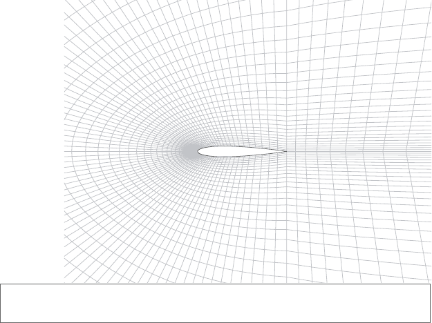
grid is shown in Figure 12.2 and it consists of 4,800 finite volume cells. The
governing equations are described by two dimensional inviscid Euler equations
thatcan beobtained fromequation (1)byremoving viscousfluxesF
v
anddropping
the momentum, continuity, and energy term in the z-direction
∂
∂t
&
Qd +
G
∂
F
c
dA = 0 (37)
Here Q and F
c
are given by
Q =
⎛
⎜
⎜
⎝
ρ
ρu
ρv
ρE
⎞
⎟
⎟
⎠
, F
c
=
⎛
⎜
⎜
⎝
ρV
ρuV + n
x
p
ρvV + n
y
p
ρHV
⎞
⎟
⎟
⎠
Sunden CH012.tex 17/8/2010 20: 31 Page 471
exploiting recursive properties of fixed point algorithms 471
Grid
Figure 12.2. Computational grid for NACA 0012 airfoil.
The numerical flux scheme used to approximatefluxes at the centroids of faces
offinitevolumesistheRoefluxdifferencesplittingscheme[1,6]withsecond-order
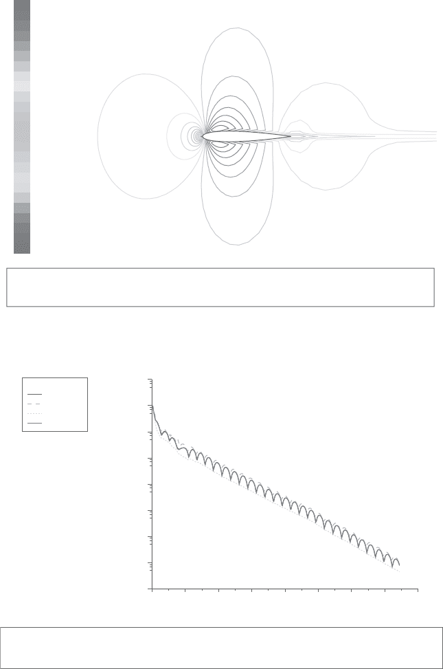
spatialaccuracy. Steadystatewasobtainedafter 375implicititerationsaccordingto
theschemeinequation(8)andwithCFLnumberequalto25.Asymmetricflowfield
pattern that wasexpected at 0
◦
angle of attackis shownin Figure 12.3. Figure 12.4
shows the convergence history of all conserved variables. Convergence behavior
is overall linear, but a small marginally unstable mode in the momentum equation
is observed that corresponds to almost a periodic half-sinusoidal oscillation of the
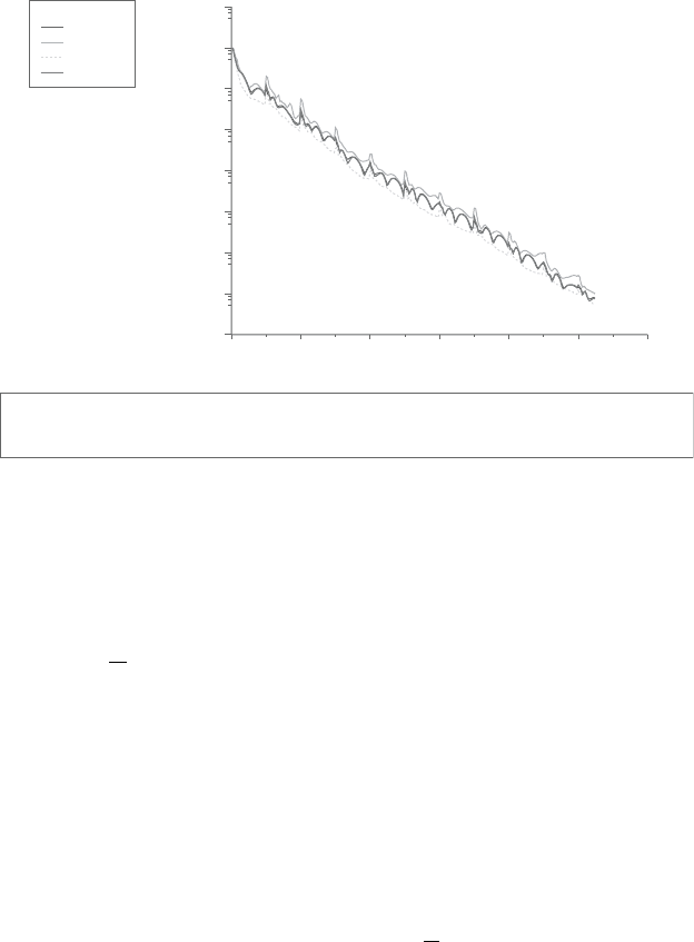
residuals. Results of the RRE algorithm that uses coupled density-based implicit
solver are shown in Figure 12.5. These results are obtained by using a size of the
restart space of 25 and it is evident from Figure 12.5 that the accelerated case
converges after 265 implicititerations of density-basedsolver. Moreover, itcan be
observed that an almost periodic marginally unstable mode evident in Figure 12.4
is no longer present and it is substituted with higher more irregular modes. The
overall savings in terms of number of iterations between baseline and accelerated
runs is about 100 iteration or 25%.
A more interesting case to consider is turbulent viscous flow over the same
NACA 0012 at an angle of attack of 1.25
◦
. For this angle of attack, a weak shock
waveappearsontheuppersurf aceoftheairfoil, closetotheleadingedge.Thebasic
set of equations, equation (1) was extended with additional turbulence transport
equations.The generic form of transport equations is given by equation (2) and in
Sunden CH012.tex 17/8/2010 20: 31 Page 472
472 Computational Fluid Dynamics and Heat Transfer
Contours of Mach number May 20, 2007
FLUENT 6.3 (2d, dp, dbns imp)
9.10eⴚ01
8.83eⴚ01
8.56eⴚ01
8.28eⴚ01
8.01eⴚ01
7.74eⴚ01
7.46eⴚ01
7.19eⴚ01
6.92eⴚ01
6.64eⴚ01
6.37eⴚ01
6.10eⴚ01
5.82eⴚ01
5.55eⴚ01
5.28eⴚ01
5.00eⴚ01
4.73eⴚ01
4.46e⫺01
4.18e⫺01
3.91e⫺01
3.64e⫺01
3.36e⫺01
3.09e⫺01
2.82e⫺01
2.54e⫺01
2.27e⫺01
Figure 12.3. Contours of Mach number for NACA 0012 airfoil at the zero angle
of attack using implicit density-based solver.
Coupled airfoil: No extrapolation
scaled residuals
May 20, 2007
FLUENT 6.3 (2d, dp, dbns imp)
Iterations
400350300250200150100500
1e⫹02
1e⫹00
1e⫺02
1e⫺04
1e⫺06
1e⫺08
1e⫺10
1e⫺12
1e⫺14
energy
y-velocity
x-velocity
continuity
Residuals
Figure 12.4. Residual history of the baseline run (no acceleration) of NACA 0012
airfoilininviscidflowatthezeroangleofattackusingimplicitdensity-
based solver.
Sunden CH012.tex 17/8/2010 20: 31 Page 473
exploiting recursive properties of fixed point algorithms 473
Coupled airfoil: With extrapolation
scaled residuals
May 20, 2007
FLUENT 6.3 (2d, dp, dbns imp)
Iterations
300250200150100500
1e⫹02
1e⫹00
1e⫺02
1e⫺04
1e⫺06
1e⫺08
1e⫺10
1e⫺12
1e⫺14
energy
y-velocity
x-velocity
continuity
Residuals
Figure 12.5. Residual history of the the accelerated run of NACA 0012 airfoil in
inviscid flow at the zero angle of attack using implicit density-based
solver.
the case of two equation turbulence model it takes the following form:
∂
∂t
&
d +
G
∂
(F
,c
− F
,v
)dA −
&
S
d = 0
Here , F
,c
, and F
,v
are given by
=
ρK
ρ!
, F
,c
=
ρKV
ρ!
∗
V
, F
,v
=
n
x
τ
K
xx
+ n
y
τ
K
yy
n
x
τ
!
xx
+ n
y
τ
!
yy
whereas S
is given by
=
P − ρ!
(C
!1
f
!1
− C
!2
f
!2
ρ!
∗
)
!
∗
K
+ φ
!
where P is production term [20] and τ
xx
and τ
yy
are normal turbulent viscous
stresses [20].The turbulence model that was used in the computation is realizable
k −! modelwiththefreestreamturbulenceconditionsthatcorrespondto0.5%tur-
bulence intensitywith a viscousratioof turbulent tolaminar viscosity of10.These
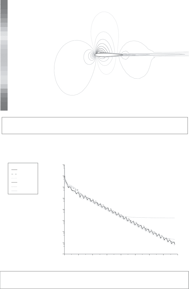
conditionscorrespond tofree streamconditions inthecalm atmosphere.Resultsof
thecomputationsusingbaselinecoupledimplicitdensity-basedsolverareshownin
Figure12.6. ConvergencebehaviorforthiscaseisshowninFigure12.7whereitcan
be seen that the convergence was achieved after 390 nonlinear iterations. It is also
Sunden CH012.tex 17/8/2010 20: 31 Page 474
474 Computational Fluid Dynamics and Heat Transfer
Contours of Mach number May 20, 2007
FLUENT 6.3 (2d, dp, dbns imp, rke)
1.01eⴙ00
9.79eⴚ01
9.47eⴚ01
9.15eⴚ01
8.84eⴚ01
8.52eⴚ01
8.20eⴚ01
7.88eⴚ01
7.56eⴚ01
7.24eⴚ01
6.93eⴚ01
6.61eⴚ01
6.29eⴚ01
5.97eⴚ01
5.65eⴚ01
5.34eⴚ01
5.02eⴚ01
4.70eⴚ01
4.38eⴚ01
4.06eⴚ01
3.75eⴚ01
3.43eⴚ01
3.11eⴚ01
2.79eⴚ01
2.47eⴚ01
2.16eⴚ01
Figure 12.6. Mach contours of NACA 0012 airfoil in viscous turbulent flow at
1.25
◦
angle of attack using implicit density-based solver.
Coupled airfoil: No extrapolation
scaled residuals
May 20, 2007
FLUENT 6.3 (2d, dp, dbns imp, rke)
Iterations
400350300250200150100500
1eⴙ02
1eⴙ00
1eⴚ02
1eⴚ04
1eⴚ06
1eⴚ08
1eⴚ10
1eⴚ12
1eⴚ14
epsilon
k
energy
y-velocity
x-velocity
continuity
Residuals
Figure 12.7. Residual history of the baseline (no acceleration) r un of NACA 0012
in viscous turbulent flow at 1.25
◦
angle of attack using implicit
density-based solver.
Sunden CH012.tex 17/8/2010 20: 31 Page 475
exploiting recursive properties of fixed point algorithms 475
observedthatturbulentdissipationrateexperiencesaplateaueffectafter200nonlin-
ear iterations,keeping thelevelof residualsat 1E–07 without any further decrease.
For practical computations, this level of residuals may be acceptable but it clearly
indicates a difficulty with the convergence of k-equation. Application of the RRE
accelerating algorithm produces better convergence behavior since the problem
converges in 275 nonlinear iterations without the plateau effect in k-equation.
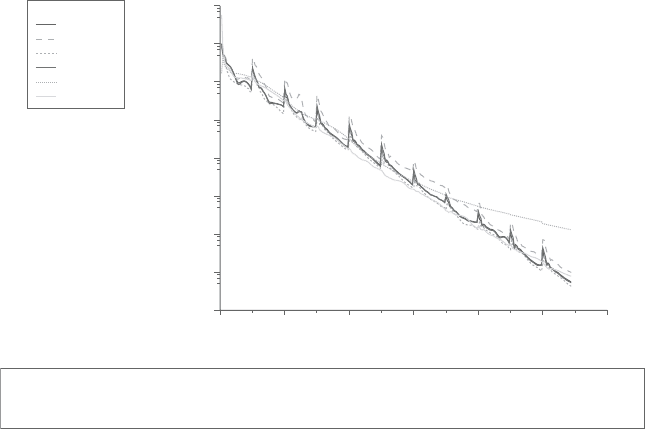
12.4.2 RRE acceleration of explicit density-based solver
HereagainweconsiderinviscidandviscousturbulentflowaroundNACA0012air-
foil at 0
◦
and 1.25
◦
angles of attack with the free-stream Mach number Ma =0.7.
However,thistimeweusetheexplicitmultistageRunge–Kuttaschemewiththefull
approximation storage scheme [1,18,19].The same set of equations, equation (37)
and the nonlinear update is performed by the explicit scheme in equation (7) with
modifications to accommodate FAS and Runge–Kutta multistage algorithms. Due
tostabilityrestrictions,CFLnumberof2isusedwithsecond-orderschemeinspace
(Figure 12.8).
ThefirstcasethatwasconsideredistheinviscidflowoverNACA0012atthezero
angle ofattack with free-stream Machnumber Ma=0.7. Convergencebehaviorof
residuals of the conserved variables are shown in Figure 12.9 where it can be seen
that it takes approximately 3,470 nonlinear iterations to reduce residuals below
tolerance level set to be 1E −12.
Coupled airfoil: With extrapolation
scaled residuals
May 20, 2007
FLUENT 6.3 (2d, dp, dbns imp, rke)
Iterations
300250200150100500
1eⴙ02
1eⴙ00
1eⴚ02
1eⴚ04
1eⴚ06
1eⴚ08
1eⴚ10
1eⴚ12
1eⴚ14
epsilon
k
energy
y-velocity
x-velocity
continuity
Residuals
Figure 12.8. Residual history of the accelerated run of NACA 0012 in viscous
turbulent flow at 1.25
◦
angle of attack using implicit density-based
solver.