Amano R.S., Sunden B. (Eds.) Computational Fluid Dynamics and Heat Transfer: Emerging Topics

Подождите немного. Документ загружается.

Sunden CH006.tex 10/9/2010 15: 39 Page 226

226 Computational Fluid Dynamics and Heat Transfer

Finally, the transformed governing equations (10–12) are written as:

Mass conservation:

∂

∂ξ

(

√

) = 0, (24)

Momentum conservation:

∂

∂t

(

√

) +

∂

∂ξ

(

√

) =−

∂

∂ξ

(

√

g(a

)

∂

∂ξ





√

∂u

∂ξ



√

(25)

Energy equation:

∂

∂t

(

√

gT)+

∂

∂ξ

(

√

T) =

∂

∂ξ



PrRe



√

∂T

∂ξ



√

(26)

Here

√

g(a

)

is the contravariant ﬂux vector where (a

)

denotes the

kth element of the vector a

, and u

the Cartesian velocity basis vector. S

and S

are additional source terms in the momentum and energy equation, respectively.

Forthefully-developedformulation,whilethemasscontinuityequationremains

unchanged, the momentum and energy equation take the form:

Momentum conservation:

∂

∂t

(

√

) +

∂

∂ξ

(

√

) =−

∂

∂ξ

(

√

g(a

)

p) +

∂

∂ξ





√

∂u

∂ξ



√

gβe

√

(27)

Energy equation:

∂

∂t

(

√

gθ) +

∂

∂ξ

(

√

θ) =

∂

∂ξ



PrRe



√

∂θ

∂ξ



−

√

gγu

−

√

∂γ

∂t

√

(28)

where Re=Re

is the Reynolds number based on the friction velocity u

∗

(Equation 13).

6.3.1 Source terms in rotating systems

Equations (24–26) are the base incompressible conservation equations in a gen-

eralized coordinate system. Additional terms due to body forces can be included

in the source terms S

and S

. In noninertial systems as that encountered in the

internal cooling of turbine blades additional Coriolis and centrifugal force terms

are included in nondimensional form:

√

=−2

√

g Ro

∈

ikm

−

√

g ∈

ilm

∈

jlk

(29)

Sunden CH006.tex 10/9/2010 15: 39 Page 227

Time-accurate techniques for turbulent heat transfer analysis 227

where Ro

is the rotation number given by ω

∗

ref

∗

ref

, ω

∗

is the component of

angular velocityin the i-direction, r

is the radialcomponent from the axis ofrota-

tion in the k-direction, and ∈

jlk

is the permutation tensor. In the case of orthogonal

rotation about one axis (say the z-axis; ω

∗

= ω

∗

=0), equation (29) reduces to

√

= 2

√

gRo

√

gRo

;

√

=−2

√

gRo

√

gRo

√

= 0

(30)

Coriolis forces have a preferential effect on turbulence, augmenting or attenu-

ating it depending on the orientation of the rotational axis with respect to the

primary strain rate in the ﬂow. The preferential effect has a profound impact

on heat transfer coefﬁcients, and ﬂuid temperatures can vary substantially in the

domain makingthe densitydifferencesnontrivial.Thedensity differencesgive rise

to differential centrifugal forces which are aptly referred to as centrifugal buoy-

ancyforces.Thisis usuallyaccommodatedbyusingthe Boussinesqapproximation

ρ

∗

/ρ

∗

ref

=−T

∗

ref

to give

√

=−2

√

gRo

∈

ikm

−

√

g ∈

ilm

∈

jlk



1 −T

∗

ref



(31)

wherethe second term in theparenthesis represents thecentrifugalbuoyancy term.

For developing and fully-developed ﬂow T

∗

ref

= T

∗

, and T

∗

= (T

∗

−T

∗

)orT

∗

ref

∗

ref

/κ

∗

for constant temperature and constant heat ﬂux boundary conditions,

respectively.

6.4 Computational Framework

Thetransformedequationscaneitherbesolvedonastaggeredornonstaggeredgrid.

Heretheequationsarediscretized andsolvedon anonstaggered grid usinga ﬁnite-

volumeapproach.The dependent variablesu, v, w, P,orp andT or θ are calculated

at the cell center, while the contravariant ﬂux vector, which is representative of the

normalﬂuxtoacoordinatesurface,isdeﬁnedandcalculatedatthecellfaces,

√

at ξ

=const. Typically, the grid metrics are calculated using appropriate second-

order central (SOC) difference approximations. If high-order accuracy is desired,

high-orderapproximationsareusedtocalculatethegridmetrics.Thecovariantbasis

vectors(a

,a

),theJacobian

√

g, thecontravariantbasisvectors(a

,a

),the

diagonal elements of the covariant metric tensor (g

), and off-diagonal

elements ofthe contravariantmetrictensor (g

) arecalculated and stored

at the cell center. Further, to calculate the contravariant ﬂuxes at the cell faces the

contravariantbasisvectorsanddiagonalelementsof thecontravariantmetrictensor

are calculated and stored at the appropriate cell face (a

at ξ

=const).

Theaboveequations arediscretizedand solved inamultiblockframework.This

is accomplishedby introducingan overlap region or ghost cellsat interblockfaces.

Typically, the overlap region is dictated by the order of discretization used in the

Sunden CH006.tex 10/9/2010 15: 39 Page 228

228 Computational Fluid Dynamics and Heat Transfer

Face

Axis 2

Axis 1

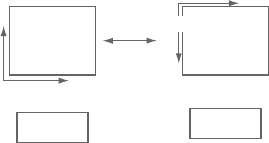
Figure 6.2. Anexampleofunstructuredblocktopology.Eastface(ξ+)ofoneblock

exchangesinformation with thenorth face (η+)ofan adjoining block.

The axes are also arbitrarily oriented with each other.

domain – for second-order discretizations, a single ghost cell region is needed at

an interblock boundary; for second-orderupwind approximationsand fourth-order

central approximations, the ghost cells increase to two and so on. Obviously, the

expected increase in accuracy has to be balanced against the increased cost of the

scheme itself, to which updating the overlap regions would addto, particularlyin a

parallel distributed computing framework.

While each block has a structured mesh, the interblock topology can either

be structured or unstructured. In a str uctured topology, a ξ

block face can only

interface with an adjoining ξ

−

block face with coordinate axes perfectly aligned

with each other on the two faces. In an unstructured topology, this restriction is

relaxed and a ξ

block face can interface with any of the six adjoining block faces

with any axesorientations. Figure 6.2 shows suchanexample in which the ξ

face

of one block interfaces with η

face of another block.

In this instance, data transferred from one face to the other has to be sorted

and realigned with the receiving coordinate system. The sorting operation is

abstracted as:



= [S]



(32)

where



A is the data-vector (of size equal to the number of nodes in the surface) to

be transferred from one face to the other and [S] is a symmetric sorting matrix.

If the elements of



A have a directional dependence on the transformed coordi-

natessuchascomponentsofthecovariantvectorsx

,x

orotherderivativesw.r.t.

ξ, η, and ζ, an additional transformation is performed. For example in Figure 6.2,



face

=−



face

.A general transformation is represented as:

⎡

⎣



⎤

⎦

face

= [S][T]

⎡

⎣



⎤

⎦

face

(33)

Sunden CH006.tex 10/9/2010 15: 39 Page 229

Time-accurate techniques for turbulent heat transfer analysis 229

where [T] is a 3×3 transformation matrix. For the example in Figure 6.2

[T] =

⎡

⎣

010

−100

001

⎤

⎦

An additional feature that is useful is the capability to handle nonconforming or

nonmatchingblockinterfaces,i.e.,whenthereisnoone-to-onematchbetweennode

locationsintwoadjoiningblockinterfaces.Thiscapabilityisusefulinzonalreﬁning

or coarsening of meshes from one block to another. In such cases, in addition to

the sorting matrix, an interpolation matrix is constructed. Consider the η

face in

Figure 6.2 to have n total nodes, which need to be transferred to ξ

face with m

nodes.Then a further generalization of equation (32) can be written as:



m×1

= []

m×n

[S]

n×n



n×1

(34)

where []isthem ×n interpolation matrix.

Theinterpolationoperatorshouldataminimumhavethesameorderofaccuracy

as the discrete approximations in the code. Bi-linear interpolation is the simplest

giving close to second-order accuracy. Higher-order methods based on quadratic

or cubic splines can also be used but at a higher cost [5]. During interpolation it is

also important to conserve the mass, momentum, and energy ﬂuxes moving across

the interface. Some elements of this are explained in Section 5.3.

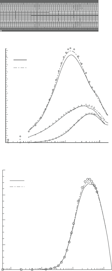
Figure6.3 shows resultsfrom a zonalmeshused for thesimulation of turbulent

channel ﬂow at Re

=180.The results are compared to the DNS data of Kim et al.

[6] (KMM). Turbulent channel ﬂow in spite of its geometrical simplicity embod-

ies all the essential characteristics of wall-bounded turbulence and is an ideal test

case for numerical developments in the simulationofturbulent ﬂow.The zones are

demarcatedat y

=50and100, withresolutions of64×14×80, 48×9×64, and

32×9×48 cells, respectively, for L

=2π and L

=π and half-channel height for

a total resolution of 226,304 cells on a six-block mesh. Because of the relatively

small-scale turbulence present in the ﬂow, it provides a stringent test case for the

treatment of nonmatching boundaries. The results are compared to a single zone

mesh of 64×64×64 or 262,144 cells. Bi-linear interpolations are used at block

boundaries, together with Dirichlet boundary conditions for pressure with the con-

servation of integrated mass ﬂux and pressure gradients across zonal boundaries.

Theoverallpredictionaccuracyissatisfactoryforthezonaldecomposition,butpeak

valuesareslightlyunderpredictedcomparedtothesinglezonemesh.Inaddition, at

the zonal boundary y

=50, the normal and shear stresses exhibit discontinuities

in slope.

Thiscanbeattributedtothehighlyenergeticsmall-scaleeddiesinthisregionand

the resultinginterpolation errors. Hence, unless high-orderinterpolations are used,

nonmatching boundaries should be used in regions where the ﬂow has relatively

large-scale features that can be captured relatively well on the grid [7].

Sunden CH006.tex 10/9/2010 15: 39 Page 230

230 Computational Fluid Dynamics and Heat Transfer

Z X

(a)

(b)

2.6

2.4

2.2

Symbols

DNS (KMM)

Zonal mesh

Single mesh

1.8

1.6

1.4

1.2

rms

, v

rms

, w

rms

0.8

0.6

0.4

0.2

rms

0.8

0.6

0.4

turbulent shear stress (−u′v′)

DNS (KMM)

Zonal mesh

Single mesh

0.2

−1

Symbols

(c)

Figure 6.3. (a) Zonal mesh in x–y plane; (b) rms quantities in wall coordinates;

interfaces are at y

=50 and 100.

Sunden CH006.tex 10/9/2010 15: 39 Page 231

Time-accurate techniques for turbulent heat transfer analysis 231

6.5 Time-IntegrationAlgorithm

A number of algorithms are available for time integration of the conservative

equations. The most common methods for incompressible ﬂow are the so-called

“pressure” based methods, which solve for pressure by formulating a pressure

equation using the mass continuity equation. Typically within this framework, the

momentumequationsareintegratedintimeusingsomeguessforthepressuregradi-

ent(fromapreviousiterateortimestep)togiveanintermediatevelocityﬁeld,which

is then made to satisfy mass continuity by correcting with the calculated pressure

ﬁeld. Whereas for steady-ﬂow calculations, algorithms based on the semi-implicit

pressure-linked equations (SIMPLE) method are quite popular (Patankar [8];

VersteegandMalalasekera [9]),for unsteady solutionsthe fractional stepapproach

ﬁnds widespread use (Ferziger and Peric [10]). Whereas methods based on the

SIMPLE algorithm solve the full set ofnonlinear equations iteratively ateach time

step and hence technically do not have any time step restrictions, methods based

on fractional step can be fully explicit with time step limited by both convective

Courant–Frederichs–Levy(CFL)condition andviscous limits(Chorin [11]),semi-

implicitinwhichonlytheviscoustermsaretreatedimplicitly(KimandMoin[12]),

and fully implicit in which both convection and viscous terms are treated implic-

itly (Choi and Moin [13]). Although time step limitations in the fractional step

approach can be an impediment to efﬁcient solution, for unsteady turbulent ﬂows

small time steps are indeed desirable to resolve the small turbulent time scales. In

fact a balanced spatio-temporal discretization dictates a CFL of O(∼1) and large

time steps can have the same undesirable effect on the solution as a coarse spatial

grid or a dissipative spatial discretization.

Here threealgorithmic implementations within thefractional step approachare

given. In the predictor step an intermediate velocityﬁeld ˜u

is computed explicitly,

semi-implicitly, or implicitly by neglecting the effect of pressure gradient. In the

explicit treatment, a second-order accurate in time Adams-Bashforth scheme is

used to approximate both the convective and viscous terms. In the semi-implicit

treatment, which is primarily used for low Reynolds number ﬂows, the viscous

terms are treated implicitly by a second-order Crank–Nicolson approximation. In

the implicit treatment, both convective and viscous terms are treated by a Crank–

Nicolson approximation. In all three methods the convection ter ms are linearized

byusing the contravariant ﬂuxes at time level n or n−1.Additionally, built into the

algorithm is the explicit conservation of surface-integrated mass, momentum, and

energyat nonmatching block interfaces, whichyield conserved variables 

√

,

u

, and T

, respectively, where  denotes conserved variables. The energy

equation needs only the predictor step to obtain T

n+1

and takes a form similar to

the equations (35)–(37) below.

6.5.1 Predictor step

First, momentum and energy ﬂuxes across nonmatching interfaces are conserved

to obtain the conserved quantity u

 or T

.

Sunden CH006.tex 10/9/2010 15: 39 Page 232

232 Computational Fluid Dynamics and Heat Transfer

Explicit formulation:

˜u

−u



t

−

n−1

(35)

where

=−

√

∂

∂ξ

(

√

u

) +

√

∂

∂ξ





√

∂u



∂ξ



+ S

Semi-implicit formulation:

˜u

−u



t

−

n−1

√

∂

∂ξ





√



∂˜u

∂ξ

∂u



∂ξ



(36)

where H

=−

√

∂

∂ξ

(

√

u

) +S

Implicit formulation:

˜u

−u



t

=−

√

∂

∂ξ



√

˜u

+

√

u



√

∂

∂ξ





√



∂˜u

∂ξ

∂u



∂ξ



+ S

(37)

where

√

−

√

n−1

is a linearized estimation of

√

The superscript

∼

denotes the intermediate ﬁeld,  denotes quantities based on

conserved ﬂuxes at nonmatching boundaries, and n the present time level. In the

semi-implicit and implicit formulation, at inhomogeneous boundaries ˜u

n+1

in the momentum equations and

T =T

n+1

are used in the energy equation. The

semi-implicit and implicit splitting of the momentum equations introduce an error

of O(t

), which is of the same order as the temporal discretization.

6.5.2 Pressure formulation and corrector step

After obtaining the intermediate Cartesian velocity ﬁeld, the continuity equationis

used to derive the pressure equation, which is then solved to obtain the pressure

ﬁeld at time (n +1)t. The calculated pressure ﬁeld is then used to correct the

intermediate velocity ﬁeld to satisfy the divergence-free condition. On a staggered

grid,thisprocedureisstraightforwardsincetheintermediatevelocitiesareavailable

onthe cellfaceof thepressure nodeand thereis noambiguity insatisfying discrete

continuity. On the other hand, on a nonstaggered grid, interpolations of nodal

velocities and pressure gradient terms are necessary at the cell face. This leads to

a discrete pressure Laplacian, which does not exhibit good ellipticity as dictated

by the continuous Laplace operator and leads to the classic problem of grid scale

Sunden CH006.tex 10/9/2010 15: 39 Page 233

Time-accurate techniques for turbulent heat transfer analysis 233

i + 1i − 1 i

i + 1/2

i + 1/2i − 1/2

Staggered

Nonstaggered

i − 1/2

i − 1

u-velocity

i + 1

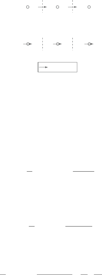
Figure 6.4. One-dimensional staggered and nonstaggered g rids.

pressureoscillations(Taftietal.[14]).Thealleviationoreliminationofthisproblem

isanimportantissueonnonstaggeredgridsand isdealtwithin somedetailhere.To

understand it better, a general framework is developed in which the nonstaggered

grid approximations are written in terms of their staggered grid counterparts.This

frameworkis thenusedtoelucidateon someof thetechniques usedin theliterature

to approach the staggered grid formulation.

Figure 6.4 shows a one-dimensional (1-D) Cartesian staggered and nonstag-

gered grid, with the locations of velocity and pressure. On a staggered grid, the

nondimensional x-momentum equation is solved at i ±1/2 location as follows:



∂u

∂t



i+1/2

=f (u) −

i+1

− p



(38)

where f (u) are the convection and viscous terms. Here, the pressure gradient term

is approximated by a compact gradient operator. On the nonstaggered grid, the

x-momentum equation with a SOC difference approximation for the pressure

gradient at location i is discretized as follows:



∂u

∂t



=f (u) −

i+1

− p

i−1

2

(39)

In this case, the pressure gradient is approximated by the noncompact form of

the gradient operator. By using Taylor series approximations, we can rewrite this

equation in a compact gradient operator form and an “error” term as follows:



∂u

∂t



= f (u) −

i+1/2

− p

i−1/2



−





∂

∂x



+ ... (40)

Inessence,thenodalmomentumequationonanon-staggeredgridhasanadditional

third derivative pressure term implicitly included in its formulation which can be

Sunden CH006.tex 10/9/2010 15: 39 Page 234

234 Computational Fluid Dynamics and Heat Transfer

written as:



∂u

∂t





∂u

∂t



−





∂

a+1

∂x

a+1



+ ... (41)

where the superscript ns refers to nonstaggered and s refers to staggered grid. In

this case a=2, and ε

=8.

In deriving the pressure equation, the 1-D equivalent of the discrete continuity

equation is of the form:

i+1/2

− u

i−1/2



= 0or







∂u

∂t



i+1/2

−



∂u

∂t



i−1/2



= 0 (42)

In the staggered grid system, u

i+1/2

and u

i−1/2

are available at the cell faces from

thex-momentumequation.However,inthenonstaggeredgrid,thesevelocitieshave

to be interpolated to the cell faces. Using second-order symmetric inter polations

for (∂u/∂t)

i+1/2

and equation (39) gives



∂u

∂t



i+1/2

(f (u)

i+1

+ f (u)

) −

i+2

+ p

i+1

− p

i−1

4

(43)

Using Taylor series expansions for f (u) about the staggered node i +1/2, and

expressing the pressure gradient term in terms of its compact form (p

i+1

−p

,),

equation (43) can be written as:



∂u

∂t



i+1/2

= f (u)

i+1/2

−

i+1

− p





∂

f (u)

∂x



i+1/2

−





∂

c+1

∂x

c+1



i+1/2

+...

(44)

or in general



∂u

∂t





∂u

∂t







∂

f (u)

∂x



−





∂

c+1

∂x

c+1



+ ... (45)

whereb=2, ε

=8,c =2, andε

=4.Equation (45)givesageneral expressionfor

the equivalent cell face momentum equation used on a nonstaggered grid in terms

of itsstaggered grid counterpart toconstruct thepressure equation.The expression

includestwoadditionalterms, oneofwhichis aresultof thecellfaceinterpolation,

andtheother,asintheexpressionforthenodalvelocity,isaresultofthenoncompact

form of the g radient operator. It is to be noted that the order of the interpolation

error term can in fact be reduced by using high-order interpolations. Zang et al.

[15] have used a QUICK type upwind biased approximation to interpolate the cell

face values which gives b=3 and ε

=24 in equation (45). However, although the

Sunden CH006.tex 10/9/2010 15: 39 Page 235

Time-accurate techniques for turbulent heat transfer analysis 235

magnitude of the error term introduced by the noncompact form of the pressure

gradient can be reduced (Tafti et al. [14]), the order of the error always remains

O(

) with the third derivative of pressure.

Finally, using the 2-D equivalent forms of equations (45) and (42) a modiﬁed

pressure equation in two dimensions is derived as:

∇





∂

c+2

∂x

c+2







∂

c+2

∂y

c+2



+ ...=

t

(∇·˜u)





∂

b+1

f (u,v)

∂x

b+1







∂

b+1

g(u,v)

∂y

b+1



+ ...

(46)

where∇

isa compactLaplacianand (∇·˜u)

isthe compactdivergenceoperator

as obtained on a staggered g rid. The constants b, c, ε

, and ε

have the same

values as in equation (45). It is clear that the extra terms in the modiﬁed pressure

equation introduce high frequency errors of O(

) into the pressure ﬁeld, which

contribute to the grid scale pressure oscillations. The elimination of the spurious

pressure terms in equation (46) has been researched extensively. For example,

Sotiropoulus andAbdallah [16] use regularizingterms in the pressure equation (of

type −



∂

∂x

,0≤ε ≤1) which partially or exactly cancel the spurious terms in

equation(46).Ina2-D-drivencavitytheyfoundthatε =0.1wassufﬁcienttoobtain

smoothpressureﬁelds.However,byarbitrarily“regularizing”thepressureequation,

discrete continuity is not exactly satisﬁed. In order to overcome this deﬁciency,

Tafti et al. [14] used equation (42) for discretizing the divergence operator in the

continuityequation,anddirectionallybiasedthepressuregradientoperatortoobtain

a discrete Laplacian that exhibited better ellipticity (L

Laplacian in reference

[14]). This Laplacian was found to eliminate pressure oscillations in a 2-D-driven

cavity and also satisﬁed discrete continuity. For this approximation, equation (39)

took the equivalent form:



∂u

∂t



= f (u) −

−p

i+2

+ 6p

i+1

− 3p

− 2p

i−1

6

(47)

resultingina=2,andε

=−24inequation(41)forthenodalmomentumequation,

b=c =2, and ε

=8 and ε

=12 in equations (45) and (46). Hence, the direction-

ally biased pressure gradient approximation was successful in reducing the error

in the spurious pressure term by a factor of 3; however, as noted previously, the

order of the error term remained the same. A limitation of this method is that the

discreteLaplacianhas alargestencil andhencemakesimplementation in ageneral

coordinate frame quite cumbersome.

An additional criterion that needs to be satisﬁed when solving the pressure

equation is the integ rability constraint. It states that the discrete pressure Poisson