Amano R.S., Sunden B. (Eds.) Computational Fluid Dynamics and Heat Transfer: Emerging Topics

Подождите немного. Документ загружается.

Sunden CH004.tex 10/9/2010 15: 9 Page 146

146 Computational Fluid Dynamics and Heat Transfer

u /u

mean

−1

Chen et al. [18]

PresentAC-CBS

Ra = 0

Ra = 10

Ra = 2x10

Ra = 5x10

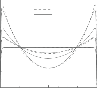
Figure 4.24. Mixed convection in porous vertical channel. Non-dimensional

vertical velocity at different Ra for aiding ﬂow, at Da=10

−4

The ﬂow enters the domain from the bottom at a non-dimensional temperature

of T =0 with a fully developed parabolic velocity proﬁle. The uniform heat ﬂux

condition is symmetrically imposed on both walls. Figure 4.23b shows the details

of the computational grid near the entrance. The mesh employed has 8,601 nodes

and 16,800 elements and it is reﬁned near the walls and at the inlet region.

Figure4.24showsthedimensionlessverticalvelocityproﬁleata Darcynumber

equalto10

−4

andfourdifferentRayleighnumbers.Thepresentresultsarecompared

with the numericalresults of Chen et al. [18]. Forpure forced convection (Ra=0),

the velocity proﬁle is ﬂat in the central part of the domain and sharply goes to

zero at the walls of the channel. In the case of aiding ﬂow, if the Rayleigh number

increases, the buoyancy forces result in an increase in the ﬂuid velocity near the

walls.As the ﬂow rate entering the channel is the same for any Rayleigh numbers

considered, the increase in ﬂuid velocity in the near-wall regions will result in a

decreased velocity at the centre region of the channel. When Rayleigh number is

increased to 5×10

, the maximum velocity inthenear-wallregion is signiﬁcantly

higher than the ﬂuid velocity at the centre of the channel.

4.2 The Finite Element Method

We provide here an introduction to weighted residual approximation and ﬁnite

element method for self-adjoint equations and for convection–diffusion equations.

4.2.1 Strong and weak forms

TheLaplaceequationisaveryconvenientexampleforthestartofnumericalapprox-

imations.Weshallgeneralizeslightlyanddiscussinsomedetailthequasi-harmonic

Sunden CH004.tex 10/9/2010 15: 9 Page 147

Applications of ﬁnite element method to heat convection problems 147

(Poisson) equation:

−

∂

∂x



∂φ

∂x



+ Q = 0 (29)

where k and Q are speciﬁed functions. These equations together with appropriate

boundary conditions deﬁne the problem uniquely.The boundary conditions can be

of Dirichlet type:

φ =

φ, on 

(30)

or that of Neumann type:

=−k

∂φ

∂n

, on 

(31)

where a bar denotes a speciﬁed quantity. Equations (29)–(31) are known as the

strong form of the problem.

We note that directuse of equation (29) requirescomputation of second deriva-

tives to solve a problem using approximate techniques. This requirement may be

weakened by considering an integral expression for equation (29) written as:





−

∂

∂x



∂φ

∂x



+ Q



d = 0 (32)

in which v is an arbitrary function.

Ifweassume equation(29) isnot zeroat somepoint x

in thenwecan alsolet

v be a positive parameter times the same value resulting in a positive result for the

integral equation (32). Since this violates the equality we conclude that equation

(29) must be zero for every x

in , hence proving its equality with equation (32).

Wemayintegratebypartsthesecondderivativetermsinequation(32)toobtain:



∂v

∂x



∂φ

∂x



d +



vQd −



∂φ

∂x



d = 0 (33)

We now split the boundary into two parts, 

and 

, with  =

+

, and

use equation (31) in equation (33) to give:



∂v

∂x



∂φ

∂x



d +



vQd −



d = 0 (34)

which is valid only if v vanishes on 

. Hence we must impose equation (30) for

equivalence.

Equation (34) is known as the weak form of the problem since only ﬁrstderiva-

tivesarenecessaryinconstructingasolution. Suchformsarethebasisforobtaining

the ﬁnite element solutions.

Sunden CH004.tex 10/9/2010 15: 9 Page 148

148 Computational Fluid Dynamics and Heat Transfer

4.2.2 Weighted residual approximation

In a weighted residual scheme, an approximation to the independent variable φ is

written as a sum of known trial functions (basis functions) N

) and unknown

parameters

.Thus we can always write:

φ ≈

φ = N

)

+ N

)

+ ...

(35)



a=1

)

= N(x

)

where

N = [N

,...N

] (36)

and

φ = [

,...,

]

(37)

In a similar way we can express the arbitrary variable v as:

v ≈ˆv = W

)˜v

+ W

)˜v

+ ...



a=1

)˜v

= W(x

)˜v (38)

in which W

are test functions and ˜v

arbitrary parameters. Using this form of

approximation will convert equation (34) to a set of algebraic equations.

In the ﬁnite element method and indeed in all other numerical procedures for

which a computer-based solution can be used, the test and trial functions will

generally be deﬁned in a local manner. It is convenient to consider each of the

tests and basis functions to be deﬁned in partitions 

of the total domain .This

division is denoted by:

 ≈ 



(39)

and in a ﬁnite element method 

are known as elements. The very simplest uses

lines in one dimension, triangles in two dimensions and tetrahedra in three dimen-

sions in which the basis functions are usually linear polynomials in each element

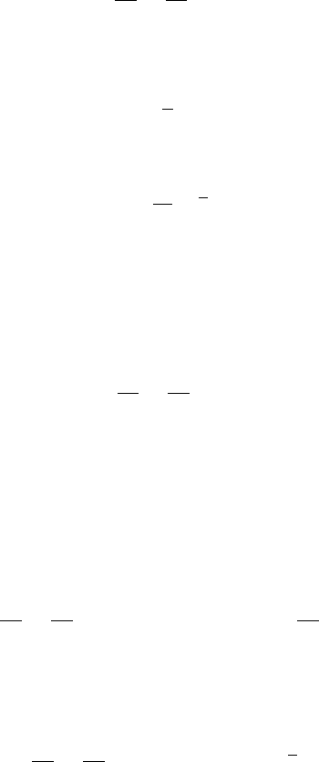
andtheunknownparametersarenodalvaluesofφ. InFigure4.25weshowatypical

set of such linear functions deﬁned in two dimensions.

In a weighted residual procedure, we ﬁrst insert the approximate function

into the governing differential equation creating a residual, R(x

), which of course

should be zero at the exact solution. In the present case for the quasi-harmonic

equation we obtain:

R =−

∂

∂x





∂N

∂x



+ Q (40)

Sunden CH004.tex 10/9/2010 15: 9 Page 149

Applications of ﬁnite element method to heat convection problems 149

∼

Figure 4.25. Basisfunctioninlinearpolynomialsforapatchoftriangularelements.

and we now seek the best values of the parameter set

, which ensures that:



Rd = 0, b = 1,2,...,n (41)

Note that this is the term multiplying the arbitrary parameter ˜v

. As noted

previously, integration by parts is used to avoid higher-order derivatives (i.e. those

greater than or equal to two) and therefore reduce the constraints on choosing the

basis functions to permit integration over individual elements using equation (39).

In the present case, for instance, the weighted residual after integration by parts

and introducing the natural boundary condition becomes:



∂W

∂x





∂N

∂x



d +



Qd +



d = 0 (42)

4.2.3 The Galerkin, ﬁnite element, method

IntheGalerkinmethod wesimplytakeW

, whichgivestheassembledsystem

of equations:



a=1

+ f

= 0, b = 1,2,...,n −r (43)

where r is the number of nodes appearing in the approximation to the Dirich-

let boundary condition (i.e., equation (30)) and K

is assembled from element

contributions K

with:



∂N

∂x

∂N

∂x

d (44)

Sunden CH004.tex 10/9/2010 15: 9 Page 150

150 Computational Fluid Dynamics and Heat Transfer

Similarly, f

is computed from the element as:



Qd +



d (45)

To impose the Dirichlet boundary condition we replace

by φ

for the r

boundary nodes.

ItisevidentinthisexamplethattheGalerkinmethodresultsinasymmetricsetof

algebraic equations (e.g. K

). However, this only happens if the differential

equations are self-adjoint. Indeed the existence of symmetry provides a test for

self-adjointness and also for existence of a variational principle whose stationarity

is sought.

It is necessary to remark here that if we were considering a pure convection

equation:

∂φ

∂x

+ Q = 0 (46)

symmetry would not exist and such equations can often become unstable if the

Galerkin method is used.

4.2.4 Characteristic Galerkin scheme for convection–diffusion equation

Unlikeasimpleconductionequation(astheLaplaceequation),anumericalsolution

for the convection equation has to deal with the convection part of the governing

equationinaddition todiffusion.For most conductionequations, the ﬁniteelement

solution is straightforward. However, if a Galerkin type approximation was used

in the solution of convection equations, the results will be marked with spurious

oscillations in space if certain parameters exceed a critical value (element Peclet

number). This problem is not unique to ﬁnite elements as all other spatial dis-

cretization techniques have the same difﬁculties.A very well-known method used

in ﬁnite elements approximation to reduce these oscillations is the Characteristic

Galerkin (CG) scheme (Lewis et al. [19], Zienkiewicz et al. [20]). Here, we follow

the Characteristic Galerkin (CG) approach to deal with spatial oscillations due to

the discretization of the convection transport terms.

In order to demonstrate the CG method, let us consider the simple convection–

diffusion equation in one dimension, namely:

∂φ

∂t

+ u

∂φ

∂x

−

∂

∂x



∂φ

∂x



= 0 (47)

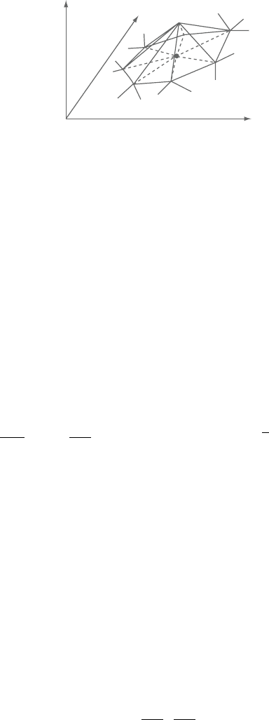
Let usconsidera characteristic of theﬂowas shown in Figure 4.26 in thetime–

space domain.The incremental time period covered by the ﬂow is t from the nth

timeleveltothe n+1thtime leveland theincremental distancecoveredduringthis

Sunden CH004.tex 10/9/2010 15: 9 Page 151

Applications of ﬁnite element method to heat convection problems 151

Characteristic

n + 1

∆t

− ∆x

∆x

− ∆x

Figure 4.26. Characteristic in a space–time domain.

timeperiodisx

,thatis, from(x

−x

)tox

.Ifamovingcoordinateisassumed

along the path of the characteristic wave with a speed of u

, the convection terms

of equation(47) disappear(as ina Lagrangian ﬂuid dynamicsapproach).Although

this approach eliminates the convection term responsible for spatial oscillation

when discretized in space, the complication of a moving coordinate system x



introduced, that is, equation (47) becomes:

∂φ

∂t



,t) −

∂

∂x





∂φ

∂x





= 0 (48)

The semi-discrete form of the above equation can be written as:

n+1

− φ

−x

t

−

∂

∂x





∂φ

∂x





−x

= 0 (49)

Notethatthediffusiontermis treatedexplicitly. It ispossibleto solvethe above

equationbyadaptingamovingcoordinatestrategy.However,asimplespatialTaylor

seriesexpansioninspaceavoidssuchamovingcoordinateapproach.Withreference

to Figure 4.26, we can write using aTaylor series expansion:

−x

= φ

−

∂φ

∂x

x

∂

∂x

x

− ... (50)

Similarly, the diffusion term is expanded as:

∂

∂x





∂φ

∂x





−x

∂

∂x



∂φ

∂x



−

∂

∂x



∂

∂x



∂φ

∂x





x (51)

Sunden CH004.tex 10/9/2010 15: 9 Page 152

152 Computational Fluid Dynamics and Heat Transfer

Figure 4.27. One-dimensional linear element.

On substituting equations (50) and (51) into equation (49), we obtain (higher-

order terms being neglected) the following expression:

n+1

− φ

t

=−

x

t

∂φ

∂x

x

2t

∂

∂x

∂

∂x



∂φ

∂x



(52)

In this case, all the terms are evaluated at position x

, and not at two positions

asinequation(49).If theﬂowvelocityis u

, we canwrite x=u

t. Substituting

into equation (52), we obtain the semi-discrete form as:

n+1

− φ

t

=−u

∂φ

∂x

+ u

t

∂

∂x

∂

∂x



∂φ

∂x



(53)

By carrying out a Taylor series expansion (Figure 4.26), the convection term

reappears inthe equationalong withan additional second-orderterm.Thissecond-

order term acts as a smoothing operator that reduces the oscillations arising from

the spatial discretization of the convection terms. The equation is now ready for

spatial approximation.

The following linear spatial approximation of the scalar variable ϕ in space is

used to approximate equation (53):

φ = N

+ N

= [N]{ϕ} (54)

where [N] are the shape functions and subscripts i and j indicate the nodes of a

linear element as shown in Figure 4.27.

On employing the Galerkin weighting to equation (53), we obtain:



[N]

n+1

− φ

t

d +



[N]

∂φ

∂x

d

(55)

−

t



[N]

∂

∂x

d −



[N]

∂

∂x



∂φ

∂x



= 0

The above equation is equal to zero only if all the element contributions are

assembled. For a domain with only one element, we can substitute:

[N]





(56)

Sunden CH004.tex 10/9/2010 15: 9 Page 153

Applications of ﬁnite element method to heat convection problems 153

On substituting a linear spatial approximation for the variable φ, over elements

as typiﬁed in Figure 4.27, into equation (55), we get:



[N]

{φ

n+1

− φ

}

t

d =−u



[N]

∂

∂x

([N]{φ})

d

(57)

t



[N]

∂

∂x

([N]{φ})

d +



[N]

∂

∂x

([N]{φ})

d

Before utilizing thelinear integration formulae, weapply Green’s lemma to the

second-order terms of equation (57), we obtain:



[N]

{φ

n+1

− φ

}

t

d =−u



[N]

∂[N]

∂x

{φ}

d

−

t



∂[N]

∂x

∂[N]

∂x

{φ}

d +

t



[N]

∂[N]

∂x

{φ}

d (58)

−



∂[N]

∂x

∂[N]

∂x

{φ}

d +



[N]

∂[N]

∂x

{φ}

d

wheren

and n

are thedirection cosinesof the outward normal n,  is thedomain

and  is the domain boundary. The ﬁrst-order convection term can be integrated

eitherdirectlyorviaGreen’slemma.Here,theconvectiontermisintegrateddirectly

without applying Green’s lemma. However, integration of the ﬁrst derivatives by

partsisusefulforproblemsinwhichthetractionisprescribed.Usingtheintegration

formulae (Lewis et al. [19]), it is possible to derive the element matrices for all the

terms in equation (58).The term on the left-hand side for a single element is:



[N]

{φ

n+1

− φ

}

t

d =





⎧

⎨

⎩

n+1

−φ

t

n+1

−φ

t

⎫

⎬

⎭

= [M

]

{ϕ}

t

(59)

where [M

] is the mass matrix for a single element. The above mass matrix for a

single element will have to beutilizedin an assembly procedure for a ﬂuid domain

containing many elements.

In a similar fashion, all other terms can be integrated; for example, the

convection term is given by:



[N]

∂[N]

∂x

{φ}

d =



−11

$

= [C

]{ϕ}

(60)

where [C

] is the elemental convection matrix.The values of the derivatives of the

shape functions are substituted in order to derive the above matrix.

Sunden CH004.tex 10/9/2010 15: 9 Page 154

154 Computational Fluid Dynamics and Heat Transfer

The diffusion term within the domain is integrated as:



∂[N]

∂x

∂[N]

∂x

{φ}

d =



1 −1

−11

$

= [K

]{ϕ}

(61)

where [K

] is the elemental diffusion matrix. The characteristic Galerkin term

within the domain is integrated as:

t



∂[N]

∂x

∂[N]

∂x

{φ}

d = u

t



1 −1

−11

$

= [K

]{ϕ}

(62)

where [K

] is the elemental stabilization matrix.

The boundary term from the diffusion operator is integrated by assuming that i

is a boundary node, as follows:



[N]

∂[N]

∂x

{φ}

d = k

⎧

⎨

⎩

−

⎫

⎬

⎭

= [f

] (63)

where {f

} is the forcing vector due to the diffusion term.

Theboundary integralfromthecharacteristic Galerkintermisintegrated,again

by assuming that i is a boundary node, as:

t



[N]

∂[N]

∂x

{φ}

d =

t

⎧

⎨

⎩

−

⎫

⎬

⎭

= [f

] (64)

where {f

} is the forcing vector due to the stabilization term.

Foraone-dimensional domainwithmore thanoneelement, allthematrices and

vectorsneedtobeassembledinordertoobtaintheglobalmatrices.Onceassembled,

the discretized one-dimensional equation becomes:

[M]

{ϕ}

t

=−[C]{φ}

− [K]{φ}

− [K

]{φ}

+{f}

+{f

}

(65)

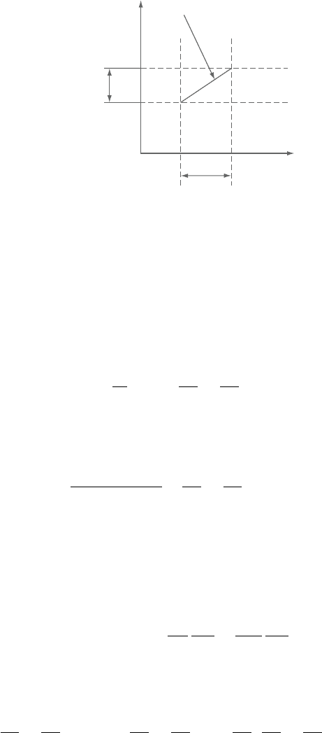
Let us now consider a simple one-dimensional convection problem, as given in

Figure 4.28, to demonstrate the effect of a discretization with and without the CG

scheme.

The scalar variable value at the inlet is ϕ =0, and at the exit its value is 1.This

scalar variable is transported in the direction of the velocity as shown in Figure

4.28. Note that the convection velocity u

is constant. The element Peclet number

for this problem is deﬁned as:

Pe =

(66)

where h is the element size in the ﬂow direction, which, in one dimension is the

local element length. Figure 4.29 shows the comparison between a solution with

Sunden CH004.tex 10/9/2010 15: 9 Page 155

Applications of ﬁnite element method to heat convection problems 155

= 0

Inlet

= constant

φ = 1

Exit

Figure 4.28. One-dimensional convection–diffusion problems.

0.8

0.6

Function

0.4

0.2

0 0.2 0.4

Horizontal distance

(a) Pe = 1.0

0.6 0.8 1

0.8

0.6

Function

0.4

0.2

0 0.2 0.4

Horizontal distance

(b) Pe = 1.5

0.6 0.8

Standard Galerkin

Characteristic Galerkin

Exact solution

Standard Galerkin

Characteristic Galerkin

Exact solution

Figure 4.29. Spatial variation of a function, φ, in one-dimensional space for

different element Peclet numbers.

the CG discretization scheme and one without it. Only two Peclet numbers are

shown in these diagrams to demonstrate the spatial oscillations without the CG

discretization. As seen, both discretizations give no spatial oscillations at a Pe

value of unity. However, at a Pe value of 1.5, the CG discretization is accurate and

stable,whilethe discretizationwithout theCG term becomesoscillatory.The exact

solution to this problem is given as follows (Brooks and Hughes [21]):

φ =

1 −e

(67)

In this equation, L is the total length of the domain and x

is the local length of

the domain.

The extension of the characteristic Galerkin scheme to a multi-dimensional

scalar convection–diffusion equation is straightforward and follows the previous

procedure as discussed for a one-dimensional case.

4.2.5 Stability conditions

The stability conditions for a given time discretization may be derived using

a Von Neumann or Fourier analysis for either the convection equation or the

convection–diffusion equations. However, for more complicated equations such