ACCA F5 Performance Management - 2010 - Study text

Подождите немного. Документ загружается.

Chapter 8: Quantitative analysis in budgeting

Time series analysis

 The nature of a time series

 Linear regression analysis and forecasting a trend line

 Moving averages

 Calculating seasonal variations

 Using the trend line and seasonal variations to make forecasts

 Problems with seasonal variation analysis

4 Time series analysis

4.1 The nature of a time series

A time series is a record of data over a period of time. In budgeting, an important

time series is the amount of annual sales revenue (or sales revenue per month or

revenue per quarter) over time. Historical data about sales might be used to predict

what sales will be in the future, in the budget period, when it is assumed that there

is an upward or downward trend over time.

Trends might be identified over time for other aspects of a business, such as the

number of people employed by the entity or the number of customer orders

handled.

There are several techniques that may be used to predict a future from historical

data for a time series. With these techniques, it is assumed that:

 There is an underlying trend, which is either an upward trend or downward

trend.

 There may be seasonal variations (or monthly variation or daily variations)

around the trend line.

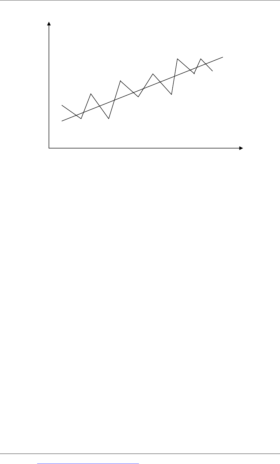
The diagram below shows a trend line with seasonal variations above and below the

trend line. The general trend in this diagram is up and the trend can be shown as a

straight line. However the actual value in each time period is above or below the

trend, because of the seasonal variations.

Paper F5: Performance management

206 Go to www.emilewoolfpublishing.com for Q/As, Notes & Study Guides © EWP

Analysing a time series

There are two aspects to analysing a time series from historical data:

 Estimating the trend line

 Calculating the amount of the seasonal variations (or monthly variations or daily

variations).

The time series can then be used to make estimates for a future time period, by

calculating a trend line value and then either adding or subtracting the appropriate

seasonal variation for that time period.

Two methods of calculating a trend line are:

 Linear regression analysis

 Moving averages.

Methods of calculating seasonal variations are explained later.

4.2 Linear regression analysis and forecasting a trend line

Linear regression analysis can be used in forecasting, if it can be assumed that there

has been a linear trend in the past, and this same linear trend will continue into the

future. For example, if sales revenue has grown at a fairly constant rate in the past, it

might be assumed that sales will continue to grow at the same rate in the future.

Linear regression analysis can be used to establish a time series and forecast future

sales.

Exactly the same method is used in forecasting as for estimating fixed and variable

costs. The trend line is a formula y = a + bx, where x is the year or month.

To simplify the arithmetic for analysing the historical data, you should number the

years 1, 2, 3, 4 and so on (or even start at year 0, and number the years 0, 1, 2, 3 and

Time

Historical data

with seasonal

variations

Trend line

Chapter 8: Quantitative analysis in budgeting

so on). This is much easier than using the actual numbers for the years 2004, 2005,

2006, 2007, 2008, 2009 and so on.

Linear regression analysis is a useful method for analysing a time series, but only if:

 a straight line trend can be assumed, and

 there are no seasonal variations in the historical data..

4.3 Moving averages

Moving averages are an alternative method to linear regression analysis for

estimating a trend line, particularly when there are seasonal variations in the data.

Moving averages are calculated as follows:

 Step 1. Decide the length of the cycle. The cycle is a number of days or weeks, or

seasons or years. For example, the cycle will be seven days when historical data

is collected daily for each day of the week. The cycle will be one year when data

is collected monthly for each month of the year, or quarterly for each season.

 Step 2. Use the historical data to calculate a series of moving averages. A moving

average is the average of all the historical data in one cycle. For example,

suppose that historical data is available for daily sales over a period Day 1 – Day

21, and there are seven days of selling each week. A moving average can be

calculated for Day 1 – Day 7. Another moving average can be calculated for Day

2 – Day 8. Another moving average can be calculated for Day 3 – Day 9, and so

on up to a moving average for Day 15 – Day 21.

 Step 3. Match each moving average with an actual time period. The moving

average should be matched with the middle time period of the cycle. For

example a moving average for Day 1 – Day 7 is matched with Day 4, which is

the middle of the period. Similarly, a moving average for Day 2 – Day 8 is

matched with Day 5, and a moving average for Day 15 – Day 21 is matched with

Day 18.

 Step 4. Use the moving averages (and their associated time periods) to calculate

a trend line, using simple averaging, the high low method or linear regression

analysis. It is also often useful to plot the data on a graph and extend a line of

best fit.

Example

A company operates for five days each week. Sales data for the most recent three

weeks are as follows:

Sales Monday Tuesday Wednesday

Thursday Friday

units units units units units

Week 1

78 83 89 85 85

Week 2

88 93 99 95 95

Week 3

98 103 109 105 105

For convenience, it is assumed that Week 1 consists of Days 1 – 5, Week 2 consists of

Days 6 – 10, and Week 3 consists of Days 11 – 15.

Paper F5: Performance management

208 Go to www.emilewoolfpublishing.com for Q/As, Notes & Study Guides © EWP

This sales data can be used to estimate a trend line. A weekly cycle in this example

is 5 days, so we must calculate moving averages for five day periods, as follows:

Period Middle day Moving average

Days 1 – 5 Day 3 [78 + 83 + 89 + 85 + 85] /5 84

Days 2 – 6 Day 4 [83 + 89 + 85 + 85 + 88] /5 86

Days 3 – 7 Day 5 [89 + 85 + 85 + 88 + 93] /5 88

Days 4 – 8 Day 6 [85 + 85 + 88 + 93 + 99] /5 90

Days 5 – 9 Day 7 [85 + 88 + 93 + 99 + 95] /5 92

Days 6 – 10 Day 8 [88 + 93 + 99 + 95 + 95] /5 94

Days 7 – 11 Day 9 [93 + 99 + 95 + 95 + 98] /5 96

Days 8 – 12 Day 10 [99 + 95 + 95 + 98 + 103] /5 98

Days 9 – 13 Day 11 [95 + 95 + 98 + 103 + 109] /5 100

Days 10 – 14 Day 12 [95 + 98 + 103 + 109 + 105] /5 102

Days 11 – 15 Day 13 [98 + 103 + 109 + 105 + 105]/5 104

In this example, all the moving average figures lie on a perfect straight line. It can be

seen that each day the trend increases by 2. If x = the day number, the formula for

the trend can be calculated by taking any day, say day 12

a + 2 × 12 = 102 so a = 78.

The formula is daily sales = 78 + 2x.

This trend line can be used to calculate the ‘seasonal variations’ (in this example the

daily variations in sales above or below the trend).

Moving averages and trend line when there is an even number of seasons

When there is an even number of seasons in a cycle, the moving averages will not

correspond to an actual season. When this happens it is necessary to take moving

averages of the moving averages, which will correspond to an actual season of the

year.

Example

The following sales figures have been recorded for a company, where sales are

known to fluctuate with the season of the year. There are four seasons (four

quarters) in the year. Historical data for quarterly sales is shown in the table below.

Sales Quarter 1 Quarter 2 Quarter 3 Quarter 4

$000 $000 $000 $000

Year 1

20 24 27 31

Year 2

35 39 44 47

Year 3

49 56 60 64

These quarters for the three years will be called Quarter 1 – Quarter 12. There are

four seasons in the annual cycle, so moving average values for each quarter are

calculated as follows:

Chapter 8: Quantitative analysis in budgeting

Period Middle quarter Moving average Moving average

of moving average

(average of 2)

Quarters 1 – 4 Quarter 2.5 25.50

Quarter 3 27.375

Quarters 2 – 5 Quarter 3.5 29.25

Quarter 4 31.125

Quarters 3 – 6 Quarter 4.5 33.00

Quarter 5 35.125

Quarters 4 – 7 Quarter 5.5 37.25

Quarter 6 39.250

Quarters 5 – 8 Quarter 6.5 41.25

Quarter 7 43.000

Quarters 6 – 9 Quarter 7.5 44.75

Quarter 8 46.875

Quarters 7 – 10 Quarter 8.5 49.00

Quarter 9 51.000

Quarters 8 – 11 Quarter 9.5 53.00

Quarter 10 55.125

Quarters 9 – 12 Quarter 10.5 57.25

The moving averages in the right hand column correspond with an actual season.

These moving averages are used to estimate the trend line and the seasonal

variations.

4.4 Calculating seasonal variations

The trend line on its own is not sufficient to make forecasts for the future. We also

need estimates of the size of the ‘seasonal’ variation for each of the different seasons.

In the two examples above:

 In the first example we need an estimate of the amount of the expected daily

variation in sales, for each day of the week.

 In the second example we need to calculate the variation above or below the

trend line for each season or quarter of the year.

A ‘seasonal variation’ can be measured from historical data as the difference

between the actual historical value for the time period, and:

 the corresponding moving average value, where moving averages are used, or

 the corresponding straight line value for the trend line, where linear regression

analysis is used.

Either of two assumptions might be made about seasonal variations.

Paper F5: Performance management

210 Go to www.emilewoolfpublishing.com for Q/As, Notes & Study Guides © EWP

 The additive assumption. This assumption is that the sum of seasonal variations

above and below the trend line in each cycle adds up to zero. Seasonal variations

below the trend line have a negative value and variations above the trend line

have a positive value. Taking all the seasonal variations together in one cycle,

they will add up to 0.

 The proportional assumption. This assumption is that the actual value in each

season can be expressed as a proportion of the trend line value. For example,

sales in Quarter 1 might be 120% of the trend line value, sales in Quarter 2 95%

of the trend line value, sales in Quarter 3 103% of the trend line value and sales

in Quarter 4 85% of the trend line value. When the proportional assumption is

used for seasonal variations, the seasonal variations in the cycle multiplied

together must = 1. In the example above, 1.20 × 0.95 × 1.03 × 0.85 = 1.0 (allowing

for a small rounding error).

Estimating seasonal variations: the additive model

The seasonal variation for each season (or daily variation for each day) is estimated

as follows, when the additive assumption is used:

 Use the moving average values that have been calculated from the historical

data, and the corresponding historical data. (‘actual’ data) for the same time

period.

 Calculate the difference between the moving average value and the actual

historical figure for each time period. This is a seasonal variation. You will now

have a number of seasonal variations, covering several weekly or annual cycles.

 Group these seasonal variations into the different seasons of the year (or days of

the week). You will now have several seasonal variations for each day of the

week or season of the year.

 For each season (or day), calculate the average of these seasonal variations.

 This average seasonal variation for each day of the week or season of the year is

used as the seasonal variation for the purpose of forecasting. However, if the

seasonal variations for the cycle do not add up to zero, adjust the seasonal

variations so that they do add up to zero.

The seasonal variations can then be used, with the estimated trend line, to make

forecasts for the future.

Chapter 8: Quantitative analysis in budgeting

Example

Using the example above of the trend line for daily sales, the seasonal variations are

calculated as follows:

Middle

day

Day of the

week

Moving

average value

Actual sales Variation

(Actual – Moving

average)

Day 3 Wednesday 84 89 + 5

Day 4 Thursday 86 85 - 1

Day 5 Friday 88 85 - 3

Day 6 Monday 90 88 - 2

Day 7 Tuesday 92 93 + 1

Day 8 Wednesday 94 99 + 5

Day 9 Thursday 96 95 - 1

Day 10 Friday 98 95 - 3

Day 11 Monday 100 98 - 2

Day 12 Tuesday 102 103 + 1

Day 13 Wednesday 104 109 + 5

The seasonal variation (daily variation) is now calculated as the average seasonal

variation for each day, as follows:

Variation Monday Tuesday Wednesday Thursday Friday

units units units units units

Week 1 + 5 - 1 - 3

Week 2 - 2 + 1 + 5 - 1 - 3

Week 3 - 2 + 1 + 5

Average - 2 + 1 + 5 - 1 - 3

Points to note

(1) In this example, the average seasonal variation for each day of the week is

exactly the same as the actual seasonal variations. This is because the historical

data in this example produces a perfect trend line.

(2)

The total of the seasonal variations for each day of the week is 0. (- 2 + 1 + 5 – 1 –

3 = 0.) When seasonal variations are applied to a straight-line trend line, they

must always add up to zero. If the seasonal variations did not add up to 0, the

trend line would not be straight. It would ‘curve’ up or down, depending on

whether the sum of the seasonal variations is positive or negative.

(3)

If the total of the seasonal variations over a cycle do not add up to 0, the

variations should be adjusted so that they do add up to 0 – for example by

adding 1 or subtracting 1 from the variation for the seasons with the largest

variations.

Paper F5: Performance management

212 Go to www.emilewoolfpublishing.com for Q/As, Notes & Study Guides © EWP

Estimating seasonal variations with the proportional model

When a proportional model is used to calculate seasonal variations, rather than the

additive model, the seasonal variations for each time period are calculated by

dividing the actual data by corresponding moving average or trend line value.

Example

Using the previous example for quarterly sales, actual sales and the corresponding

moving average value were as follows:

Quarter

Actual sales in

the quarter

Moving average

value of sales

Seasonal variation:

actual sales as a

proportion of the

moving average

Year 1, Quarter 3 27 27.375 0.986

Year 1, Quarter 4 31 31.125 0.996

Year 2, Quarter 1 35 35.125 0.996

Year 2, Quarter 2 39 39.250 0.994

Year 2, Quarter 3 44 43.000 1.023

Year 2, Quarter 4 47 46.875 1.003

Year 3, Quarter 1 49 51.000 0.961

Year 3, Quarter 2 56 55.125 1.016

Variation Quarter 1 Quarter 2 Quarter 3 Quarter 4

Year 1 0.986 0.996

Year 2 0.996 0.994 1.023 1.003

Year 3 0.961 1.016

Average 0.978 1.004 1.004 0.999

Adjust to 0.98 1.01 1.01 1.00

In this example, the seasonal variations are very small. The average variation for

each quarter is found by multiplying the values for the variations, and taking the

nth root. In quarter 1 for example, the average variation is calculated as √ (0.996 ×

0.961) = 0.978.

The adjustment is made so that the seasonal variations, when multiplied together,

come to 1.0.

In this example, the seasonal variations are very small.

Chapter 8: Quantitative analysis in budgeting

4.5 Using the trend line and seasonal variations to make forecasts

When the trend line and seasonal variations have been estimated, we can make

forecasts for the future. In the example above of daily sales, suppose that we wanted

to forecast sales in units each day during Week 4 (days 16 – 20) and the trend line is

78 + 2x.

The ‘seasonal variations’ (daily variations) are as calculated above: - 2, + 1, + 5, - 1

and - 3.

The daily sales forecasts are calculated as follows:

Day Trend line value

(78 + 2x)

Seasonal

variation

Forecast

sales

(units)

16 Monday 110 - 2 108

17 Tuesday 112 + 1 113

18 Wednesday 114 + 5 119

19 Thursday 116 - 1 115

20 Friday 118 - 3 115

4.6 Problems with seasonal variation analysis

There are two problems with using this technique to make forecasts with seasonal

variations.

(1)

The historical data will not provide a perfect trend line. The trend line that is

estimated with the historical data is a ‘best estimate’, not a perfect estimate.

(2)

It is assumed that seasonal variations are a constant value, whereas they

might be changing over time.

(3)

Forecasts using estimated trends and seasonal variations are based on the

assumptions that the past is a reliable guide to the future. This assumption

may be incorrect. However, forecasts must be made; otherwise it is impossible

to make plans beyond the very short term.

Estimates based on judgement and experience

There is an argument that instead of using models to forecast future sales (or make

any other time series forecast), it might be better to rely on the judgement and

experience of management.

Management will be aware of changes in the business environment or in the market

that might affect results in the future, and time series analysis based on moving

averages and seasonal variations would not make any allowance for these expected

changes.

However, the drawback to relying on management judgement is that managers can

make incorrect guesses.

Paper F5: Performance management

The learning curve

 Learning curve theory: the learning effect

 The learning curve model

 Graph of the learning curve

 Formula for the learning curve

 Conditions for the learning curve to apply

5 The learning curve

5.1 Learning curve theory: the learning effect

When a team of workers begins a skilled task for the first time, and the task then

becomes repetitive, they will probably do the job more quickly as the workers learn

the task and so become more efficient. They will find quicker ways of performing

tasks, and will become more efficient as their knowledge and understanding

increase. This improvement in efficiency through experience is called the learning

effect.

When a skilled task is well-established and has been in operation for a long time, the

learning effect wears out, and the time to complete the task eventually becomes the

same every time the task is subsequently carried out.

When the average time to produce an additional unit becomes constant, a ‘

steady

state’

has been reached.

However, during the learning period, the time to complete each subsequent task can

fall by a very large amount and the earning effect can be substantial.

The learning effect (and learning curve) was first discovered in the US during the

1940s, in aircraft manufacture. It probably still applies today in aircraft manufacture.

Aircraft manufacture is a highly-skilled task, where:

 the skill of the work force is important, and

 the labour time is a significant element in production resources and production

costs.

Where the learning effect is significant, it has implications for:

 costs of completing the task, and

 budgeting/forecasting production requirements and production costs

 pricing the output so as to make a profit.

Prices charged to the customer can allow for the cost savings that will be made

because of the learning effect

ACCA F5 Performance Management - 2010 - Study text - Emile Woolf Publishing

Подождите немного. Документ загружается.