Zdunkowski W., Trautmann T., Bott A. Radiation in the atmosphere: A course in Theoretical Meteorology
Подождите немного. Документ загружается.


9.5 Mie’s scattering problem 345
so that we finally obtain the orthogonality relations for the n functions in the
form
2π
0
π
0
n
e
o,mn
· n
e
o,mn
sin ϑdϑdϕ =π
(1 + δ
0,m
)
(1 − δ
0,m
)
2n(n + 1)
(2n + 1)
2
(n + m)!
(n − m)!
×{(n + 1)
[
z
n−1
(kr )
]
2
+ n
[
z
n+1
(kr )
]
2
}
(9.57)
The orthogonality relations involving mixed products of the m and n functions
may be obtained in the same way as described above. A detailed derivation of the
corresponding relations is given by Stratton (1941). For completeness we list the
additional orthogonality relations
2π
0
π
0
m
e
o,mn
· n
e
o,ml
sin ϑdϑdϕ = 0
2π
0
π
0
m
e
o,mn
· n
o
e,ml
sin ϑdϑdϕ = 0
2π
0
π
0
m
e
o,mn
· m
o
e,ml
sin ϑdϑdϕ = 0
2π
0
π
0
n
e
o,mn
· n
o
e,ml
sin ϑdϑdϕ = 0
(9.58)
9.5 Mie’s scattering problem
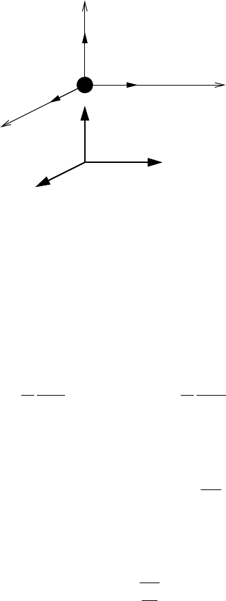
We are now prepared to discuss the actual scattering problem. Given is a spherical
particle of radius a which is embedded in a vacuum. This particle is illuminated by
a plane electromagnetic wave of wavelength λ. We assume that the wave is linearly
polarized and propagating in the positive z-direction. It is traditional to designate
the direction of the electric vector as the direction of polarization.
1
The task at hand
is to determine the scattered electromagnetic field.
9.5.1 The incoming wave
The center of the particle is located at the origin of the coordinate system and the
incoming electric vector E
i
is directed along the x-axis as shown in Figure 9.3.
1
A detailed treatment of the effects of polarization on radiative transfer will be given in the next chapter.
346 Light scattering theory for spheres
x
y
z
E
i
H
i
e
x
e
y
e
z
Fig. 9.3 Mie’s scattering problem: the incoming wave.
Again assuming a harmonic time dependency, the field vectors can be described
by
E
i
= e
x
E
i
0
exp
[
i(k
0
z − ωt)
]
, H
i
= e
y
H
i
0
exp
[
i(k
0
z − ωt)
]
(9.59)
whereby (e
x
, e
y
) are the unit vectors in (x, y)-direction. E
i
and H
i
satisfy the vector
wave equations
∇
2
E
i
−
1
c
2
∂
2
E
i
∂t
2
= 0, ∇
2
H
i
−
1
c
2
∂
2
H
i
∂t
2
= 0 (9.60)
We will now attempt to express E
i
and H
i
by means of the vectors M and N.
Substituting (9.10) into (9.1) yields
∇×E = iωB, ∇×B =−iω
N
2
c
2
E (9.61)
where (9.2) and the defining expression of the complex index of refraction N (9.7)
have been used.
For brevity we introduce the vector B
∗
by means of
B
∗
= cB =
%
µ
0
ε
0
H (9.62)
so that (9.61) assumes the form
∇×E = ik
0
B
∗
, ∇×B
∗
=−ik
0
N
2
E (9.63)
with k
0
= ω/c. Furthermore, according to (9.9), E and B
∗
fulfill the vector wave
equations
∇
2
E + k
2
0
N
2
E = 0, ∇
2
B
∗
+ k
2
0
N
2
B
∗
= 0 (9.64)

9.5 Mie’s scattering problem 347
By comparing (9.63) with (9.43), utilizing (9.42) and (9.62), it is seen that the field
vectors of the incoming wave may be written as
E
i
= E
i
0
(M
v
− iN
u
), H
i
=−H
i
0
(M
u
+ iN
v
) with H
i
0
=
%
ε
0
µ
0
E
i
0
(9.65)
In order to apply the boundary conditions to the scattering sphere, we introduce
the spherical coordinates (ϑ, ϕ, r) by means of the well-known transformation
equations
x = r sin ϑ cos ϕ, y = r sin ϑ sin ϕ, z = r cos ϑ (9.66)
The relations between the unit vectors (e
x
, e
y
, e
z
) of the Cartesian system and
(e
ϑ
, e
ϕ
, e
r
) of the spherical coordinate system are
e
ϑ
= cos ϑ cos ϕe
x
+ cos ϑ sin ϕe
y
− sin ϑe
z
e
ϕ
=−sin ϕe
x
+ cos ϕe
y
e
r
= sin ϑ cos ϕe
x
+ sin ϑ sin ϕe
y
+ cos ϑe
z
e
x
= sin ϑ cos ϕe
r
+ cos ϑ cos ϕe
ϑ
− sin ϕe
ϕ
e
y
= sin ϑ sin ϕe
r
+ cos ϑ sin ϕe
ϑ
+ cos ϕe
ϕ
e
z
= cos ϑe
r
− sin ϑe
ϑ
(9.67)
A detailed derivation of these relations may be found, for instance, in Zdunkowski
and Bott (2003). Replacing in (9.59) e
x
and e
y
by the corresponding expressions in
(9.67) yields
(9.68)
(a) E
i
= E
i
0
exp
[
i(k
0
r cos ϑ − ωt)
]
(sin ϑ cos ϕe
r
+ cos ϑ cos ϕe
ϑ
− sin ϕe
ϕ
)
(b) H
i
= H
i
0
exp
[
i(k
0
r cos ϑ − ωt)
]
(sin ϑ sin ϕe
r
+ cos ϑ sin ϕe
ϑ
+ cos ϕe
ϕ
)
The representation of the field vectors as stated in (9.65) and (9.68) shall now be
harmonized by writing series expressions for E
i
and H
i
in terms of still unknown
expansions coefficients A
mn
, B
mn
, C
mn
and D
mn
. Recalling (9.47) we may write
E
i
= E
i
0
∞
n=0
n
m=0
(
A
mn
m
mn
+ B
mn
n
mn
)
exp(−iωt)
H
i
= H
i
0
∞
n=0
n
m=0
(
C
mn
m
mn
+ D
mn
n
mn
)
exp(−iωt)
(9.69)
Comparison of coefficients of the terms involving the cos ϕ and sin ϕ functions in
(9.68), in view of the defining equations (9.48) and (9.54) for m and n, shows that
unless m =1 the coefficients A
mn
, B
mn
, C
mn
and D
mn
vanish. For this reason the

348 Light scattering theory for spheres
sums over m may be evaluated in (9.69) yielding
(a) E
i
= E
i
0
∞
n=0
A
n
m
o,1n
+ B
n
n
e
1n
exp(−iωt)
(b) H
i
= H
i
0
∞
n=0
C
n
m
e
1n
+ D
n
n
o,1n
exp(−iωt)
(9.70)
with A
1n
= A
n
, B
1n
= B
n
, C
1n
= C
n
and D
1n
= D
n
. The reason that either the
odd or the even parts of the m and n functions occur in (9.70) results from the
comparison of the cos ϕ and the sin ϕ terms appearing in (9.68) with (9.48) and
(9.54).
In order to determine the expansion coefficients A
n
, B
n
, C
n
and D
n
we make
use of the orthogonality relations (9.52) and (9.57) of the m and n functions. We
will demonstrate how to proceed by determining A
n
. The remaining coefficients
are found analogously.
First we set (9.68a) equal to (9.70a). Then we multiply both sides by the func-
tion m
o,1l
and integrate the resulting expression over the unit sphere. Thus we
obtain
2π
0
π
0
exp(ik
0
r cos ϑ)(sin ϑ cos ϕe
r
+cos ϑ cos ϕe
ϑ
−sin ϕe
ϕ
) · m
o,1l
sin ϑdϑdϕ
=
2π
0
π
0
A
n
m
o,1n
· m
o,1l
sin ϑdϑdϕ
(9.71)
Due to the orthogonality relations of the trigonometric functions, see (9.51), and
by using (9.52) we first find
π z
n
(k
0
r)
π
0
exp(ik
0
r cos ϑ)
cos ϑ
sin ϑ
P
1
n
(cos ϑ) +
dP
1
n
dϑ
sin ϑdϑ
= A
n
z
2
n
(k
0
r)2π
n(n + 1)
2n + 1
(n + 1)!
(n − 1)!
(9.72)
Recalling the relationship between the associated and the ordinary Legendre poly-
nomials
P
m
n
(x) = (1 − x
2
)
m/2
d
m
dx
m
P
n
(x) (9.73)
we may replace the expression in parenthesis on the left-hand side of (9.72) by
cos ϑ
sin ϑ
P
1
n
(cos ϑ) +
dP
1
n
dϑ
=−(1 − x
2
)
d
2
P
n
dx
2
+ 2x
dP
n
dx
= n(n + 1)P
n
(x) with x = cos ϑ
(9.74)

9.5 Mie’s scattering problem 349
where we have made use of Legendre’s differential equation
(1 − x
2
)
d
2
P
n
dx
2
− 2x
d
dx
P
n
+ n(n + 1)P
n
(x) = 0 (9.75)
Thus we obtain
A
n
=
1
z
n
(k
0
r)
2n + 1
2n(n + 1)
π
0
exp(ik
0
r cos ϑ)P
n
(cos ϑ) sin ϑdϑ (9.76)
which contains the unspecified spherical Bessel function z
n
(k
0
r). We choose z
n
= j
n
which is defined by means of
j
n
(k
0
r) =
i
−n
2
π
0
exp(ik
0
r cos ϑ)P
n
(cos ϑ) sin ϑdϑ (9.77)
The function j
n
is known as the spherical Bessel function of the first kind which is
finite at the origin. This spherical Bessel function is related to the ordinary Bessel
function of the first kind by
j
n
(k
0
r) =
%
π
2k
0
r
J
n+1/2
(k
0
r) (9.78)
Introducing (9.77) into (9.76) gives the final form of the expansion coefficient A
n
A
n
= i
n
2n + 1
n(n + 1)
, B
n
=−iA
n
, C
n
=−A
n
, D
n
= B
n
(9.79)
The remaining expansion coefficients are also stated as part of this equation. Thus
(9.70) can be rewritten as
E
i
= E
i
0
∞
n=0
i
n
2n + 1
n(n + 1)
m
o,1n
− in
e
1n
exp(−iωt)
H
i
=−H
i
0
∞
n=0
i
n
2n + 1
n(n + 1)
m
e
1n
+ in
o,1n
exp(−iωt)
(9.80)
Due to the choice z
n
= j
n
the solutions (u
n
,v
n
) of the scalar wave equation
appearing in the M and N functions for the incoming wave can be written down
immediately. From (9.37), including the factor i
n
(2n + 1)/n(n + 1) in the definition
of the u
n
and v
n
functions, we obtain
u
i
n
(r,ϑ,ϕ,t) = i
n
2n + 1
n(n + 1)
cos ϕ P
1
n
(cos ϑ) j
n
(k
0
r) exp(−iωt )
v
i
n
(r,ϑ,ϕ,t) = i
n
2n + 1
n(n + 1)
sin ϕ P
1
n
(cos ϑ) j
n
(k
0
r) exp(−iωt )
(9.81)

350 Light scattering theory for spheres
In view of equations (9.47) we may thus write the series expressions for the field
vectors of the incoming wave as
E
i
= E
i
0
∞
n=0
M
v
i
n
− iN
u
i
n
, H
i
=−H
i
0
∞
n=0
M
u
i
n
+ iN
v
i
n
with H
i
0
=
%
ε
0
µ
0
E
i
0
(9.82)
9.5.2 The scattered and the interior waves
A periodic wave which is incident on the particle gives rise to a forced oscillation
of free and bound charges synchronous with the applied field. These motions of the
charge set up a secondary field both inside and outside of the particle. The resultant
field at any point is the vector sum of the primary and the secondary fields. After
the transient oscillations are damped out a steady-state situation will occur which
will now be investigated.
As the incident wave interacts with the particle, the induced secondary field must
be constructed in two parts. The interior part of the sphere we will call transmitted (t)
while the other part, denoted by (s), refers to scattering. In analogy to the structure
of the incident field vectors we now use the forms
E
s,t
= E
i
0
∞
n=0
M
v
s,t
n
− iN
u
s,t
n
, H
s,t
=−H
s,t
0
∞
n=0
M
u
s,t
n
+ iN
v
s,t
n
with H
s
0
=
E
i
0
µ
0
c
= H
i
0
, H
t
0
=
N E
i
0
µc
(9.83)
In contrast to the incoming wave, for the wave functions u
s
n
and v
s
n
of the scattered
field we select z
n
= h
n
where h
n
are the spherical Hankel functions of the first kind.
The reason for this particular choice is the asymptotic behavior of the spherical
Hankel functions. For large values of the argument we have
h
1
n
(k
0
r) ∼
exp(ik
0
r)
k
0
r
(−i)
n+1
(9.84)
If this expression is multiplied by the factor exp(−iωt) it represents an outgoing
spherical wave (of amplitude 1), as required for the scattered wave. Thus, analo-
gously to (9.81) we may write
u
s
n
(r,ϑ,ϕ,t) = i
n
2n + 1
n(n + 1)
a
s
n
cos ϕ P
1
n
(cos ϑ)h
1
n
(k
0
r) exp(−iωt )
v
s
n
(r,ϑ,ϕ,t) = i
n
2n + 1
n(n + 1)
b
s
n
sin ϕ P
1
n
(cos ϑ)h
1
n
(k
0
r) exp(−iωt )
(9.85)

9.5 Mie’s scattering problem 351
For the inside wave we choose the function j
n
(N k
0
r) because the refractive index
is finite and the spherical Bessel function is finite at the origin. This results
in
u
t
n
(r,ϑ,ϕ,t) = i
n
2n + 1
n(n + 1)
a
t
n
cos ϕ P
1
n
(cos ϑ) j
n
(N k
0
r) exp(−iωt )
v
t
n
(r,ϑ,ϕ,t) = i
n
2n + 1
n(n + 1)
b
t
n
sin ϕ P
1
n
(cos ϑ) j
n
(N k
0
r) exp(−iωt )
(9.86)
with 0 ≤r ≤a. For the calculation of the unknown coefficients a
s,t
n
and b
s,t
n
we apply
the boundary conditions at the spherical surface which have been derived in Section
9.3. Replacing in (9.20) the unit normal vector n by e
r
we obtain
e
r
× (E
i
+ E
s
) = e
r
× E
t
, e
r
× (H
i
+ H
s
) = e
r
× H
t
(9.87)
The boundary conditions at the particle’s surface r = a can now be written down
for the various components of the M and N functions
(a)
M
v
i
n
− iN
u
i
n
ϑ
+
M
v
s
n
− iN
u
s
n
ϑ
=
M
v
t
n
− iN
u
t
n
ϑ
(b)
M
v
i
n
− iN
u
i
n
ϕ
+
M
v
s
n
− iN
u
s
n
ϕ
=
M
v
t
n
− iN
u
t
n
ϕ
(c)
M
u
i
n
+ iN
v
i
n
ϑ
+
M
u
s
n
+ iN
v
s
n
ϑ
=
N µ
0
µ
M
u
t
n
+ iN
v
t
n
ϑ
(d)
M
u
i
n
+ iN
v
i
n
ϕ
+
M
u
s
n
+ iN
v
s
n
ϕ
=
N µ
0
µ
M
u
t
n
+ iN
v
t
n
ϕ
(9.88)
Let us examine in detail equation (9.88a). Using (9.45) we obtain at r =a
1
sin ϑ
∂
∂ϕ
v
i
n
+ v
s
n
− v
t
n
−
i
k
0
r
∂
2
∂r ∂ϑ
ru
i
n
+ru
s
n
−
ru
t
n
N
= 0 (9.89)
Employing the required equations (9.81), (9.85) and (9.86) we find at r = a
N a
s
n
ρ
0
h
1
n
(ρ
0
)
= a
t
n
[
ρ j
n
(ρ)
]
− N
[
ρ
0
j
n
(ρ
0
)
]
b
s
n
h
1
n
(ρ
0
) = b
t
n
j
n
(ρ) − j
n
(ρ
0
) with
[
ρ
0
j
n
(ρ
0
)
]
=
d
dρ
0
[
ρ
0
j
n
(ρ
0
)
]
r =a
,
ρ
0
h
1
n
(ρ
0
)
=
d
dρ
0
ρ
0
h
1
n
(ρ
0
)
r =a
[
ρ j
n
(ρ)
]
=
d
dρ
[
ρ j
n
(ρ)
]
r =a
, ρ
0
= k
0
r, ρ = N ρ
0
(9.90)
Had we used the azimuthal components we would have obtained the same result.
With the help of (9.88c,d) we can obtain two additional relations for the coefficients

352 Light scattering theory for spheres
a
n
and b
n
. Altogether we find
a
t
n
[
ρ j
n
(ρ)
]
− N a
s
n
ρ
0
h
1
n
(ρ
0
)
= N
[
ρ
0
j
n
(ρ
0
)
]
µ
0
N a
t
n
j
n
(ρ) − µa
s
n
h
1
n
(ρ
0
) = µj
n
(ρ
0
)
µ
0
b
t
n
[
ρ j
n
(ρ)
]
− µb
s
n
ρ
0
h
1
n
(ρ
0
)
= µ
[
ρ
0
j
n
(ρ
0
)
]
b
t
n
j
n
(ρ) − b
s
n
h
1
n
(ρ
0
) = j
n
(ρ
0
)
(9.91)
from which the coefficients a
n
and b
n
of the scattered wave can be calculated as
a
s
n
=−
µj
n
(ρ
0
)
[
ρ j
n
(ρ)
]
− N
2
µ
0
j
n
(ρ)
[
ρ
0
j
n
(ρ
0
)
]
µh
1
n
(ρ
0
)
[
ρ j
n
(ρ)
]
− N
2
µ
0
j
n
(ρ)
ρ
0
h
1
n
(ρ
0
)
b
s
n
=−
µ
0
j
n
(ρ
0
)
[
ρ j
n
(ρ)
]
− µj
n
(ρ)
[
ρ
0
j
n
(ρ
0
)
]
µ
0
h
1
n
(ρ
0
)
[
ρ j
n
(ρ)
]
− µj
n
(ρ)
ρ
0
h
1
n
(ρ
0
)
(9.92)
The coefficients a
s
n
and b
s
n
are of paramount importance for the Mie computations.
The evaluation of the Mie expressions in some cases may pose numerical
difficulties. In order to avoid these see, for example, Deirmendjian (1969). It is
possible to state (9.92) in a somewhat simplified form by introducing the so-called
Riccati–Bessel functions which differ from the spherical Bessel functions. For
details see van de Hulst (1957). Moreover, equations (9.92) simplify by setting
µ = µ
0
which is permissible if the scattering particle is non-magnetic.
The transmission coefficients have not been stated explicitly. They are also
of great importance for the calculation of the electromagnetic energy of a scat-
tering sphere. This is, for instance, necessary if photochemical reactions within
water drops are calculated. A detailed analysis of this topic is given by Bott and
Zdunkowski (1987).
We will now return to equation (9.85) and replace the spherical Hankel function
by its asymptotic expression (9.84). Thus we find for the wave functions of the
scattered wave
u
s
n
(r,ϑ,ϕ,t) =−i
2n + 1
n(n + 1)
a
s
n
cos ϕ
k
0
r
P
1
n
(cos ϑ)exp
[
i(k
0
r − ωt)
]
v
s
n
(r,ϑ,ϕ,t) =−i
2n + 1
n(n + 1)
b
s
n
sin ϕ
k
0
r
P
1
n
(cos ϑ)exp
[
i(k
0
r − ωt)
]
(9.93)
The following abbreviations will be introduced
π
n
(cos ϑ) =
P
1
n
(cos ϑ)
sin ϑ
=
dP
n
d cos ϑ
τ
n
(cos ϑ) =
dP
1
n
dϑ
= cos ϑπ
n
(cos ϑ) − sin
2
ϑ
dπ
n
d cos ϑ
(9.94)

9.5 Mie’s scattering problem 353
where we have used (9.74). First let us treat the components of the field vectors of
the scattered wave. According to (9.83) they are given by
E
s
ϑ
=E
i
0
∞
n=0
M
v
s
n
− iN
u
s
n
ϑ
, E
s
ϕ
=E
i
0
∞
n=0
M
v
s
n
− iN
u
s
n
ϕ
, E
s
r
=−iE
i
0
∞
n=0
N
u
s
n
r
H
s
ϑ
=−H
i
0
∞
n=0
M
u
s
n
+ iN
v
s
n
ϑ
, H
s
ϕ
=−H
i
0
∞
n=0
M
u
s
n
+ iN
v
s
n
ϕ
, H
s
r
=−H
i
0
∞
n=0
i
N
v
s
n
r
(9.95)
Employing (9.45) and (9.46) we may write for the horizontal components
E
s
ϑ
= E
i
0
∞
n=0
1
sin ϑ
∂v
s
n
∂ϕ
−
i
k
0
r
∂
2
ru
s
n
∂r ∂ϑ
E
s
ϕ
= E
i
0
∞
n=0
−
∂v
s
n
∂ϑ
−
i
k
0
r sin ϑ
∂
2
ru
s
n
∂r ∂ϕ
H
s
ϑ
=−H
i
0
∞
n=0
1
sin ϑ
∂u
s
n
∂ϕ
+
i
k
0
r
∂
2
rv
s
n
∂r ∂ϑ
H
s
ϕ
=−H
i
0
∞
n=0
−
∂u
s
n
∂ϑ
+
i
k
0
r sin ϑ
∂
2
rv
s
n
∂r ∂ϕ
(9.96)
The r-component of the scattered field is proportional to r
−2
so that it may be
ignored at large distances from the scattering center.
Inserting (9.93) into (9.96) and using the definitions (9.94) we find
E
s
ϑ
=−E
i
0
cos ϕ
∞
n=1
2n + 1
n(n + 1)
a
s
n
τ
n
(cos ϑ) + b
s
n
π
n
(cos ϑ)
i
k
0
r
exp
[
i(k
0
r − ωt)
]
E
s
ϕ
= E
i
0
sin ϕ
∞
n=1
2n + 1
n(n + 1)
a
s
n
π
n
(cos ϑ) + b
s
n
τ
n
(cos ϑ)
i
k
0
r
exp
[
i(k
0
r − ωt)
]
H
s
ϑ
=−H
i
0
sin ϕ
∞
n=1
2n + 1
n(n + 1)
a
s
n
π
n
(cos ϑ) + b
s
n
τ
n
(cos ϑ)
i
k
0
r
exp
[
i(k
0
r − ωt)
]
H
s
ϕ
=−H
i
0
cos ϕ
∞
n=1
2n + 1
n(n + 1)
a
s
n
τ
n
(cos ϑ) + b
s
n
π
n
(cos ϑ)
i
k
0
r
exp
[
i(k
0
r − ωt)
]
(9.97)
Inspection of these equations shows that the following relations hold
H
s
ϑ
=−
%
ε
0
µ
0
E
s
ϕ
, H
s
ϕ
=
%
ε
0
µ
0
E
s
ϑ
(9.98)
354 Light scattering theory for spheres
Incident wave
Scattered wave
Scattering plane
x
y
l
r
l
r
z
E
i
E
s
e
ϑ
ϑ
e
ϕ
l
0
r
0
ϕ
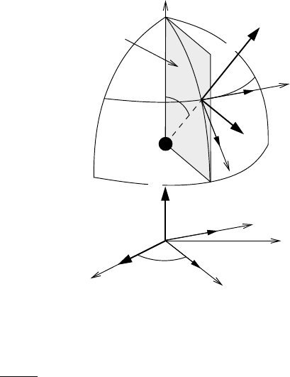
Fig. 9.4 The (l, r, z)-coordinate system and the scattering plane.
since H
i
0
=
√
ε
0
/µ
0
E
i
0
, see (9.82). For this reason, in the following it is sufficient
to discuss the electric field only.
In order to treat scattering of electromagnetic waves on spherical particles it is
advantageous to introduce the so-called (l, r)-system. For the incoming wave the
new system is obtained by rotating the original (x, y, z)-system about the z-axis in
counterclockwise direction by the angle ϕ. For the scattered wave the directions
of the l- and r -axes agree with the directions ϑ and ϕ of the spherical coordinate
system. Thus the l-axes are located in the plane defined by the directions of the
incoming and the scattered wave. This particular plane is called the scattering
plane. Figure 9.4 depicts the directions of the l- and r-axes as well as the scattering
plane. The labels l and r are taken from the last letters of the words ‘parallel’ and
‘perpendicular’ describing the directions of the components of the electric field
vectors with respect to the scattering plane.
If l
0
and r
0
are unit vectors along the l and r axis of the incident wave, according
to Figure 9.4 we may express E
i
as
E
i
= E
i
l
l
0
+ E
i
r
r
0
= E
i
0
cos ϕ exp
[
i(k
0
z − ωt)
]
l
0
− E
i
0
sin ϕ exp
[
i(k
0
z − ωt)
]
r
0
(9.99)