Yang X.-S. Introductory Mathematics for Earth Scientists

Подождите немного. Документ загружается.

170 Chapter 11. Ordinary Differential Equations

and

= h

(1 − e

−t

/τ

), (11.98)

we have

− h

= h

−t

/τ

− e

−t

/τ

), (11.99)

− h

)

−t

/τ

− e

−t

)

. (11.100)

If we take the ratio of (11.97) to (11.98), we have

1 − e

−t

/τ

1 − e

−t

/τ

, (11.101)

which can be solved to get τ by numerical methods such as the Newton-

Raphson method, to be introduced in the ﬁnal chapter. Mathemati-

cally, this is achievable, but in practice, it is very diﬃcult to determine

and t

accurately. However, we can indeed measure the diﬀerence

∆t = t

− t

accurately. In this cas e , the better alternative is to use

the rate r = dh/dt of the uplift rather than the uplift itself.

By diﬀerentiating the solution (11.94), we have

−t/τ

. (11.102)

Again two observations of rates r

and r

at two diﬀerent times t

and

, respectively, we have

−t

/τ

, r

−t

/τ

, (11.103)

whose ratio becomes

−t

/τ

−t

/τ

= e

−t

)/τ

= e

∆t/τ

. (11.104)

Taking logarithms and r e arranging the equation, we have

τ =

∆t

ln(r

)

− t

)

ln(r

)

. (11.105)

This is a more useful formula to determine the response timescale.

Alternatively, if we know τ and the current uplift rate, we can pre-

dict the uplift in the future. We know the cur rent uplift rate in the year

2000 in north Europe is about r

2000

= 0.9 cm/year. If we us e τ = 5500

years, we can estimate the uplift rate in the year 30 00. Therefore,

∆t = 1000 years. From (11.104), we have

2000

3000

= e

∆t/τ

= e

1000/5500

≈ 1.199, (11.106 )

which means

3000

2000

1.199

≈

0.9

1.199

≈ 0.75 cm/ year. (11 .107)

Chapter 12

Partial Di ﬀerential

Equations

Ordinary diﬀerential equatio ns are sometimes complicated enough, but

their applications are often limited as they only involve a single inde-

pendent variable. In e arth sciences, quantities usually depend on many

other variables, and the gove rning equations for many ge ophysical and

geological processes are often express e d in terms of par tial diﬀerential

equations (PDEs). PDEs are much more complicated than ordinary

diﬀerential equations . Here we will brieﬂy introduce the fundamentals

of PDEs and focus on the linear heat conduction and diﬀusion equation

which are of importance in earth sciences.

While introducing the basics of PDEs, we will focus on the applica-

tion of PDEs to the heat transfer process modelling, outlining Kelvin’s

estimate of the a ge of the Earth, and the general solution of the cooling

of the lithosphere.

12.1 Introduction

A partial diﬀerential equation is a relationship or equation containing

one or more partial derivatives. Similar to the ordinary diﬀerential

equation, the highest nth partial derivative is referred to as the order

n of the partial diﬀerential equation. In general, we can write it as a

generic function φ

φ(u, x, y,

∂u

∂x

∂u

∂y

∂

∂x

∂

∂y

∂

∂x∂y

, ...) = 0, (12.1)

where u is the dependent variable, and x, y, ... are the independent

variables.

171

172 Chapter 12. Partial Differential Equations

For example, the one-dimensional wave equation

∂

∂t

= v

∂

∂x

, (1 2.2)

is a second-order partial diﬀerential equation. Here time t and space x

are two independent variables, and u is the displacement. The constant

v is the wave speed. In ma ny mathematical books, compact subscript

forms are often used to denote partial derivatives for simplicity and

clarity. That is u

≡

∂u

∂x

, u

≡

∂

∂x

, u

≡

∂u

∂y

, u

≡

∂

∂x∂y

, and so on

and so forth. Using such compact notations, the wave equation can be

written as

= v

. (12.3)

12.2 Classic Equations

There ar e diﬀerent types of PDEs, and the three basic types for two

independent variables are based on the following general linear e quation

∂

∂x

+ b

∂

∂x∂y

+ c

∂

∂y

= f(x, y, u, u

, u

), (12.4 )

where a, b and c are known functions of x and y. In the simplest cases,

they can all be constants. Similar to the case of quadratic equations,

we deﬁne ∆ = b

− 4ac.

If ∆ > 0, the partial diﬀere ntial equation is said to be hyperbolic.

The wave equation

∂

∂t

= v

∂

∂x

, (1 2.5)

is a good example if we let t = y, a = v

, b = 0 and c = −1. This

means ∆ = 4v

> 0 and the equation is hyperbolic.

If ∆ < 0, the PDE is said to be elliptic. The Laplace equation

∂

∂x

∂

∂y

= 0, (12.6 )

is elliptic be c ause ∆ = −4 < 0 due to a = c = 1 and b = 0.

If ∆ = 0, the PDE is said to be parabolic. The heat conduction

equation

∂u

∂t

= κ

∂

∂x

, (12.7)

is parabolic as a = κ, c = 0 for t = y and b = 0 so that ∆ = 0.

These three types are the most commonly used in mathematical

modelling. There are other types such as the mixed type, as the coef-

ﬁcient functions depend on x and y, and in diﬀerent regions , they may

12.3 Heat Conduction 173

take diﬀerent values and the sign of ∆ will change, and subsequently

the type of the equation will also change.

The classiﬁca tion of PDEs will usually provide some information

about how the partial diﬀerential equation behaves, and we can expect

certain behaviour and characteristics of the solution of our interest. For

example, the wave equation, as the name s uggests, will support certain

travelling waves such as the vibrations of a n e lastic string, and the

acoustic vibrations of the air. In fact, almost all hyperbolic equa tions

will support some forms of waves under appropriate conditions. On the

other hand, for the parabolic equatio ns when ∆ = 0, the solution will

be smooth and any initial irregularity in the proﬁle will be smoothed

out. This is typically the behaviour of diﬀusion and heat conduction.

For example, the sug ar concentration in a cup of coﬀee will tend to

become uniform after some time, a nd the temperature of a swimming

pool will tend to be uniform to some degree. In the rest of this chapter,

we will discuss the heat conduction equation in more detail as it is very

impo rtant in earth sciences.

There are many methods for solving partial diﬀerential equations,

including separation of va riables, Fourier transforms, Laplace trans-

form, Green’s functions, s imila rity variables, spectral methods, and

others. In the rest of this chapter, we will only introduce the solution

of heat conduction eq uations and its application in the modelling of

the cooling process of lithosphere.

12.3 Heat Conduction

Suppo se we are interested in the cooling of the lithosphere. In this

case, we are only interested in the one-dimensional case of how the

temper ature T varies with time t and the depth z (see Fig. 12.1). We

know that the governing equation is the classic heat conduction

∂T

∂t

= κ

∂

∂z

, (12.8)

where κ = K/ρc

is the thermal diﬀusivity, and K is the heat conduc-

tivity. ρ is the density of the lithosphere and c

is the speciﬁc heat

capacity. The domain of our interest consists of t ≥ 0 a nd 0 ≤ z < ∞.

The boundary condition at z = 0 is that the temperature is con-

stant. That is, T = T

at z = 0. The temperature at the other

boundary where z → ∞ should approa ch the temperature T

of the

underlying mantle. In this problem, we can assume that the initial

temper ature is T (z, t = 0) = T

. We know that κ has a unit of m

/s,

so κt has a unit of m

. This means that

√

κt deﬁnes a length as its unit

is m. Therefore, the ratio z/

√

κt is dimensio nless, which is convenient

174 Chapter 12. Partial Differential Equations

T =T

lithosphere

T → T

Figure 12.1: Heat conduction in 1D.

for mathematical analysis. In fact, we c an deﬁne a similarity varia ble

ζ =

√

4κt

, (12.9)

where the fa c tor 4 is purely for convenience to avoid a factor 1/2 ap-

pearing everywhere in the end equation. Now we have T (z, t) = f(ζ).

Using the chain rules of diﬀerentiations

∂f

∂z

∂f

∂ζ

∂z

√

4κt

∂f

∂ζ

∂

∂z

∂ζ

∂z

∂ζ

∂z

∂

∂ζ

√

4κt

)

∂

∂ζ

4κt

∂

∂ζ

and

∂f

∂t

∂f

∂ζ

∂t

√

4κ

(−

−3/2

)

∂f

∂ζ

−z

√

4κt

∂f

∂ζ

= −

∂f

∂ζ

, (12.10)

we can write the origina l PDE (12.8) as

−

4κt

, (12.11)

where we have used f

dζ

∂f

∂ζ

and f

dζ

∂

∂ζ

because

f(ζ) depends on ζ only, and the pa rtial derivatives and the standard

derivatives are the same.

The above equation can be rearr anged as

= −2ζ. (12.12)

The chain rule of diﬀerentiation implies that (ln y(x))

= (1/y(x))y

(x).

Replacing y(x) by f

or letting y(x) = f

, we have (ln f

)

= f

Integrating the above equation once, we get

ln f

= −ζ

+ C, (12.13)

where C is the constant of integration. This again can be written as

= Ke

−ζ

, (12.14)

12.3 Heat Conduction 175

1 2 3−1−2−3−4

0.5

1.0

−0.5

−1.0

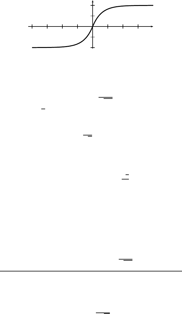
erf(x)

Figure 12.2: Plot of the error function erf(x).

where K = e

is a constant. Integrating this with resp e c t to ζ, we

have

T = f(ζ) = Aerf(

√

4κt

) + B, (12.15)

where A = K

√

π/2. Here A and B are two undeter mined constants.

The error function is deﬁned by

erf(x) =

√

−ζ

dζ. (12.16)

From its deﬁnition, we know that erf(0) = 0. At inﬁnity, we have

erf(∞) → +1, as x → +∞, erf(∞) → −1, as x → −∞. (12.17)

We know these are true because

∞

−x

dx =

√

Using the boundary condition T = T

at z = 0, we have

A erf(0) + B = T

, (12.18)

which gives B = T

. From the far ﬁeld boundary T = T

as z → ∞,

we have

A erf(∞) + B = A + B = T

. (12.19)

In combination with B = T

, we have A = T

− T

. Therefore, the

ﬁnal solution for the temperature proﬁle becomes

T (z, t) = T

+ (T

− T

)erf(

√

4κt

). (12.20)

Example 12.1: William Thomson (later Lord Kelvin) was the ﬁrst to

estimate the age of the Earth from physical principles. By assuming that

the E arth is a half-space with the condition that the tem perature tends

to T

at inﬁnite depth z → ∞, the solution o f the te m perature can be

written

T = T

erf



√

κt



176 Chapter 12. Partial Differential Equations

where z is the depth, and erf(ζ) i s the error function. Using ζ =

√

κt

and dT/dζ = d[

√

−ζ

dζ]/dζ =

√

−ζ

[see (12.23)], the thermal

gradient can be calcu lated by

G =

∂T

∂z

∂T

∂ζ

∂z

√

−ζ

√

κt

√

πκt

−ζ

At the Earth’s surface z = 0 and ζ = 0, we have G =

√

πκt

, and the heat

ﬂux Q = −K

∂T

∂z



z=0

= −

√

πκt

. We k n ow the observed heat ﬂux Q or

temperature gradient today; the age of the Earth is

t ≈

/G)

πκ

Kelvin in 1863 used the measured values at that time κ ≈ 1.2 × 10

−6

/s, T

= 3900

◦

C, and G = 36

◦

C/km=0.036

◦

C/m, he estimated that

t =

(3900/0.036)

π × 1.2 × 10

−6

≈ 3.1 × 10

seconds ≈ 98.7 Ma,

where we ha ve used 1 Ma = 1, 000, 000 × 365 × 24 × 3600 = 3.15 ×

seconds. Taking account of the uncertainties of these measurements,

Kelvin set a limit of 24 Ma to 400 Ma o n the age of the Earth. Obviousl y,

this greatly underestimate d the age of the Earth, but such calculatio n s

were a signiﬁ c a n t progress at that time.

12.4 Cooling of the Lithosphere

Now we investigate further in modelling the cooling process of the litho-

sphere near the mid-ocean ridge (see Fig. 12.3).

The solution to a heat conduction problem in a semi-inﬁnite domain

usually takes the form

T = T

+ (T

− T

)erf



√

κt



, (12.21)

where T

is the temperature at z = 0, and T

is the temperature of

the mantle.

The thermal gradient at z = 0 can be calculated by

q = −K

∂T

∂z

= −K

∂T

∂ζ

∂z

. (12.22)

Since

∂ζ

∂z

√

κt

and

∂erf(ζ)

∂ζ

√

∂

∂ζ

−u

√

−ζ

, (12.23)

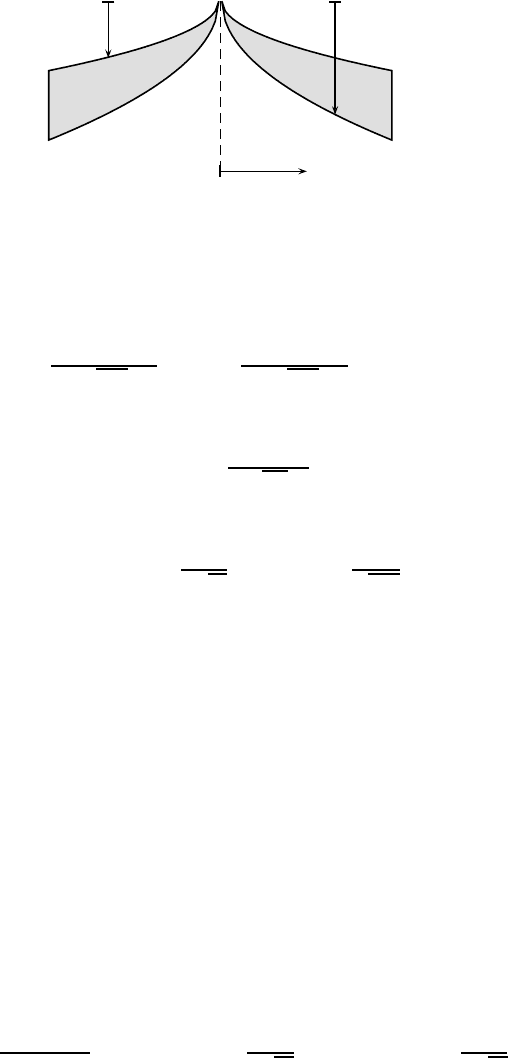
12.4 Cooling of the Lithosphere 177

Figure 12.3: Cooling and depth variations of the lithosphere

near the mid-ocean ridge.

we have

q = −

K(T

− T

)

√

πκt

−ζ

= −

K(T

− T

)

√

πκt

−z

/4κt

. (12.24)

The negative sign highlights the fact that the heat ﬂow is upwards in

the opposite direction of z. We are concerned with the value at z = 0,

therefore we have q

= q



z=0

= −

K(T

−T

)

√

πκt

For practical application, we can set T

= 0 for the Earth if we use

T in degrees, not in terms of the absolute temperature. Then, we have

T = T

erf



√

κt



, q

= −

√

πκt

. (12.25)

For a given time t, we c an estimate the heat ﬂux. Conversely, if we

know the value of the heat ﬂux, we can estimate the age of the litho-

sphere. This equation is also the basis fo r the ﬁrst estimation of the

age of the Earth by Lord Kelvin. In addition, we can also estimate the

temper ature T

once we know the a ge and the hea t ﬂux.

It is observed that the depths of the ocea n near the mid-ocean ridge

vary with time and also the distance from the ridge. The depth varia-

tions d(t) relative to the depth of the mid-ocean ridge d

are adjusted

according to the isostatic bala nce between the mass deﬁciency caused

by (ρ

− ρ

)gd and the density increase by the cooling of the litho-

sphere at any z = L and L → ∞. Here ρ

and ρ

are the densities of

the mantle and water, respectively. That is

(ρ

− ρ

)g(d − d

) +

αρ

(T − T

)gdz = 0, (12.26)

where α is the coeﬃcient of thermal expansion. Using (12.21), we have

d=d

(ρ

− ρ

)

−T

)erfc



√

κt



dz =d

+Λ

erfc



√

κt



dz,

178 Chapter 12. Partial Differential Equations

where Λ =

α(T

−T

)

(ρ

−ρ

)

, and erfc is the complementary error function,

deﬁned as erfc(ζ) = 1 − erf(ζ). In order to integrate

erfc



√

κt



dz,

we now use the integration by parts for the ca se of L → ∞

I =

∞

erfc



√

κt



dz.

Let v

= 1 and u = erfc



√

κt



, we have v = z and

∂erfc



√

κt



∂z

∂[1 − erf



√

κt



]

∂z

= −

√

πκt

−ζ

. (12.27)

We then have

I =

∞

erfc



√

κt



dz =

zerfc



√

κt

i

∞

− (−

√

πκt

)

∞

−ζ

dz.

Since erfc(∞) = 1 − erf(∞) = 0, z/2

√

κt = ζ and dζ = dz/2

√

κt, we

have

I = 0 +

√

κt

√

∞

ζe

−ζ

dζ. (12.28)

Using the integral

∞

−y

dy =

∞

−y

d(y

) =

− e

−y

∞

, (12.29)

we have

I =

√

κt

√

κt

√

. (12.30)

Therefore, we ﬁnally have the solution

d = d



2Λ

κt



= d

2αρ

− T

)

(ρ

− ρ

)

κt

. (12.31)

This is the Parsons-Sclater formula for ba thymetry. Using the typical

values of T

= 0

◦

C, κ = 8 ×10

−7

/s, T

= 1350

◦

C, α = 3 ×10

−5

/C,

= 3000 kg/m

, ρ

= 1025 kg/m

, and d

= 2500 m, we have

d = 2500 +

2 × 3 × 10

−5

× 3000 × (13 50 − 0)

(3000 − 1025)

8 × 10

−7

√

= 2500 + 6.209 × 10

−5

√

t, (12.32)

where t is in se c onds. If we convert it to the unit of million years,

we have to multiply a factor of 36 5 × 24 × 3600 × 10

= 3.15 × 10

Therefore, the ﬁnal formula becomes

d = 2500 + 6.209 × 10

−5

3.15 × 10

t ≈ 2500 + 348.5

√

t, (12.33)

where t is in Ma. This formula is almost the same as the best ﬁt to

bathymetry data d = 2500 + 350

√

t for t < 70 Ma.

Chapter 13

Geostatistics

Statistics, especially geostatistics is a n important toolset for earth sci-

ences. It concerns the data collection and interpretation, analysis and

characterisation of numerical data and design and analysis of sampling.

In this chapter, we will brieﬂy introduce the fundamentals of statis-

tics. We will then apply the introduced techniques to study the prop-

agation of errors, linear regression of earthquake data, and Brownian

motion including diﬀusion process.

13.1 Random Variables

13.1.1 Probability

When we conduct an experiment such as tossing a coin or recording the

outside noise level, we are dealing with the outcomes of the experiment.

For the tossing of a coin, there are only two poss ible outcomes: heads

(1) or tails (0). If we toss 2 coins at the same time, we want to see how

many heads may appe ar. If we use X

(i = 1, 2 ) to represent the values

of the outcomes of the two coins, we have

+ X

, (13.1)

to represent the number of heads. Here X

are the random variables.

Since they only take discrete values 0 and 1, they are also called discrete

random variables. Other examples of discrete random variables include

the numb e r of cars passing through a junction in a day, the number of

phone calls you received in a week, the number of major earthquakes

in the world in a year, and the number of rock samples you collected

during a ﬁeld trip.

On the other hand, the noise level Y can take any values within

a certain range. This random variable is called a continuous random

179