Wooldridge - Introductory Econometrics - A Modern Approach, 2e
Подождите немного. Документ загружается.


Remember that unbiasedness is a feature of the sampling distributions of
ˆ
1
and
ˆ
0
,
which says nothing about the estimate that we obtain for a given sample. We hope that,
if the sample we obtain is somehow “typical,” then our estimate should be “near” the
population value. Unfortunately, it is always possible that we could obtain an unlucky
sample that would give us a point estimate far from
1
, and we can never know for sure
whether this is the case. You may want to review the material on unbiased estimators in
Appendix C, especially the simulation exercise in Table C.1 that illustrates the concept
of unbiasedness.
Unbiasedness generally fails if any of our four assumptions fail. This means that it
is important to think about the veracity of each assumption for a particular application.
As we have already discussed, if Assumption SLR.4 fails, then we will not be able to
obtain the OLS estimates. Assumption SLR.1 requires that y and x be linearly related,
with an additive disturbance. This can certainly fail. But we also know that y and x can
be chosen to yield interesting nonlinear relationships. Dealing with the failure of (2.47)
requires more advanced methods that are beyond the scope of this text.
Later, we will have to relax Assumption SLR.2, the random sampling assumption,
for time series analysis. But what about using it for cross-sectional analysis? Random
sampling can fail in a cross section when samples are not representative of the under-
lying population; in fact, some data sets are constructed by intentionally oversampling
different parts of the population. We will discuss problems of nonrandom sampling in
Chapters 9 and 17.
The assumption we should concentrate on for now is SLR.3. If SLR.3 holds, the
OLS estimators are unbiased. Likewise, if SLR.3 fails, the OLS estimators generally
will be biased. There are ways to determine the likely direction and size of the bias,
which we will study in Chapter 3.
The possibility that x is correlated with u is almost always a concern in simple
regression analysis with nonexperimental data, as we indicated with several examples
in Section 2.1. Using simple regression when u contains factors affecting y that are also
correlated with x can result in spurious correlation: that is, we find a relationship
between y and x that is really due to other unobserved factors that affect y and also hap-
pen to be correlated with x.
EXAMPLE 2.12
(Student Math Performance and the School Lunch Program)
Let math10 denote the percentage of tenth graders at a high school receiving a passing
score on a standardized mathematics exam. Suppose we wish to estimate the effect of
the federally funded school lunch program on student performance. If anything, we
expect the lunch program to have a positive ceteris paribus effect on performance: all
other factors being equal, if a student who is too poor to eat regular meals becomes eli-
gible for the school lunch program, his or her performance should improve. Let lnchprg
denote the percentage of students who are eligible for the lunch program. Then a simple
regression model is
math10
0
1
lnchprg u, (2.54)
Chapter 2 The Simple Regression Model
51
d 7/14/99 4:31 PM Page 51

where u contains school and student characteristics that affect overall school performance.
Using the data in MEAP93.RAW on 408 Michigan high schools for the 1992–93 school
year, we obtain
mat
ˆ
h10 32.14 0.319 lnchprg
n 408, R
2
0.171
This equation predicts that if student eligibility in the lunch program increases by 10 per-
centage points, the percentage of students passing the math exam falls by about 3.2 per-
centage points. Do we really believe that higher participation in the lunch program actually
causes worse performance? Almost certainly not. A better explanation is that the error term
u in equation (2.54) is correlated with lnchprg. In fact, u contains factors such as the pover-
ty rate of children attending school, which affects student performance and is highly corre-
lated with eligibility in the lunch program. Variables such as school quality and resources are
also contained in u, and these are likely correlated with lnchprg. It is important to remem-
ber that the estimate 0.319 is only for this particular sample, but its sign and magnitude
make us suspect that u and x are correlated, so that simple regression is biased.
In addition to omitted variables, there are other reasons for x to be correlated with
u in the simple regression model. Since the same issues arise in multiple regression
analysis, we will postpone a systematic treatment of the problem until then.
Variances of the OLS Estimators
In addition to knowing that the sampling distribution of
ˆ
1
is centered about
1
(
ˆ
1
is
unbiased), it is important to know how far we can expect
ˆ
1
to be away from
1
on aver-
age. Among other things, this allows us to choose the best estimator among all, or at
least a broad class of, the unbiased estimators. The measure of spread in the distribu-
tion of
ˆ
1
(and
ˆ
0
) that is easiest to work with is the variance or its square root, the stan-
dard deviation. (See Appendix C for a more detailed discussion.)
It turns out that the variance of the OLS estimators can be computed under
Assumptions SLR.1 through SLR.4. However, these expressions would be somewhat
complicated. Instead, we add an assumption that is traditional for cross-sectional analy-
sis. This assumption states that the variance of the unobservable, u, conditional on x,is
constant. This is known as the homoskedasticity or “constant variance” assumption.
ASSUMPTION SLR.5 (HOMOSKEDASTICITY)
Var(u兩x)
2
.
We must emphasize that the homoskedasticity assumption is quite distinct from
the zero conditional mean assumption, E(u兩x) 0. Assumption SLR.3 involves the
expected value of u, while Assumption SLR.5 concerns the variance of u (both condi-
tional on x). Recall that we established the unbiasedness of OLS without Assumption
SLR.5: the homoskedasticity assumption plays no role in showing that
ˆ
0
and
ˆ
1
are
unbiased. We add Assumption SLR.5 because it simplifies the variance calculations for
Part 1 Regression Analysis with Cross-Sectional Data
52
d 7/14/99 4:31 PM Page 52

ˆ
0
and
ˆ
1
and because it implies that ordinary least squares has certain efficiency prop-
erties, which we will see in Chapter 3. If we were to assume that u and x are indepen-
dent, then the distribution of u given x does not depend on x, and so E(u兩x) E(u) 0
and Var(u兩x)
2
. But independence is sometimes too strong of an assumption.
Because Var(u兩x) E(u
2
兩x) [E(u兩x)]
2
and E(u兩x) 0,
2
E(u
2
兩x), which means
2
is also the unconditional expectation of u
2
. Therefore,
2
E(u
2
) Var(u), because
E(u) 0. In other words,
2
is the unconditional variance of u, and so
2
is often called
the error variance or disturbance variance. The square root of
2
,
, is the standard
deviation of the error. A larger
means that the distribution of the unobservables affect-
ing y is more spread out.
It is often useful to write Assumptions SLR.3 and SLR.5 in terms of the condi-
tional mean and conditional variance of y:
E(y兩x)
0
1
x. (2.55)
Var( y兩x)
2
. (2.56)
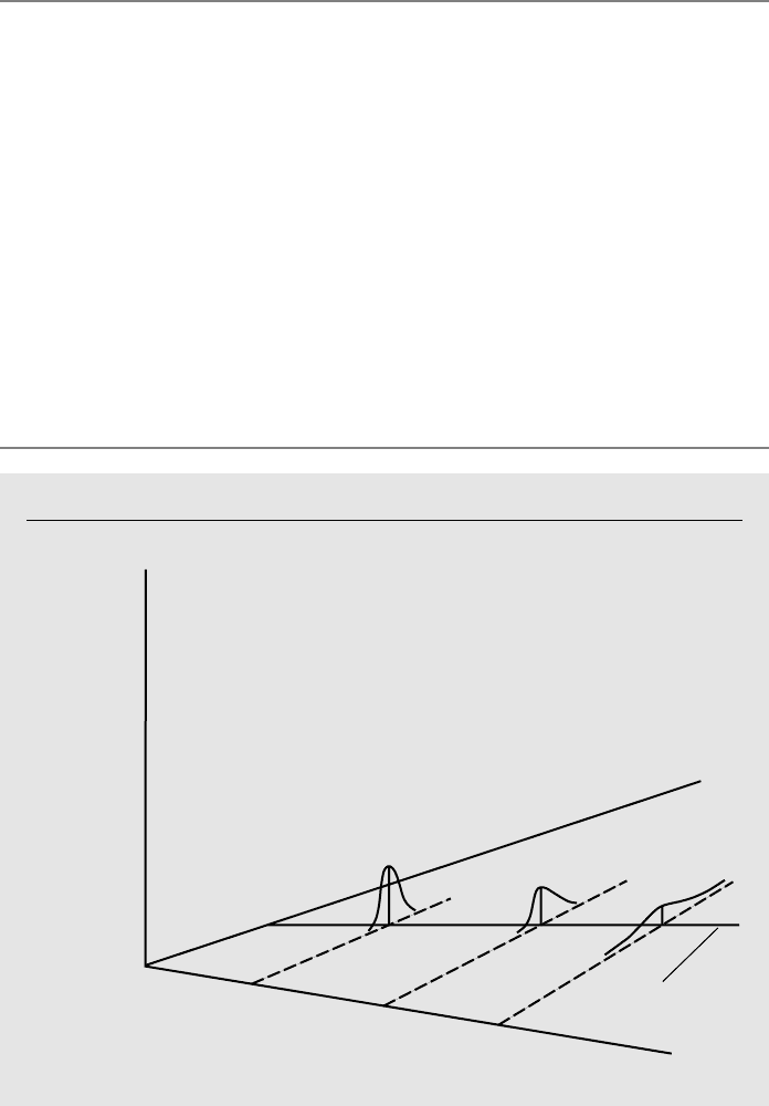
In other words, the conditional expectation of y given x is linear in x, but the variance of
y given x is constant. This situation is graphed in Figure 2.8 where
0
0 and
1
0.
Chapter 2 The Simple Regression Model
53
Figure 2.8
The simple regression model under homoskedasticity.
x
1
x
2
x
E(yx)
0
1
x
f(yx)
x
3
y
d 7/14/99 4:31 PM Page 53
When Var(u兩x) depends on x, the error term is said to exhibit heteroskedasticity (or
nonconstant variance). Since Var(u兩x) Var(y兩x), heteroskedasticity is present when-
ever Var(y兩x) is a function of x.
EXAMPLE 2.13
(Heteroskedasticity in a Wage Equation)
In order to get an unbiased estimator of the ceteris paribus effect of educ on wage, we
must assume that E(u兩educ) 0, and this implies E(wage兩educ)
0
1
educ. If we also
make the homoskedasticity assumption, then Var(u兩educ)
2
does not depend on the
level of education, which is the same as assuming Var(wage兩educ)
2
. Thus, while aver-
age wage is allowed to increase with education level—it is this rate of increase that we
are interested in describing—the variability in wage about its mean is assumed to be con-
stant across all education levels. This may not be realistic. It is likely that people with more
education have a wider variety of interests and job opportunities, which could lead to
more wage variability at higher levels of education. People with very low levels of educa-
tion have very few opportunities and often must work at the minimum wage; this serves
to reduce wage variability at low education levels. This situation is shown in Figure 2.9.
Ultimately, whether Assumption SLR.5 holds is an empirical issue, and in Chapter 8 we will
show how to test Assumption SLR.5.
Part 1 Regression Analysis with Cross-Sectional Data
54
Figure 2.9
Var (wage兩educ) increasing with educ.
8
12
educ
E(wageeduc)
0
1
educ
f(wageeduc)
16
wage
d 7/14/99 4:31 PM Page 54

With the homoskedasticity assumption in place, we are ready to prove the fol-
lowing:
THEOREM 2.2 (SAMPLING VARIANCES OF THE
OLS ESTIMATORS)
Under Assumptions SLR.1 through SLR.5,
Var(
ˆ
1
)
2
/s
x
2
(2.57)
Var(
ˆ
0
) , (2.58)
where these are conditional on the sample values {x
1
,…,x
n
}.
PROOF: We derive the formula for Var(
ˆ
1
), leaving the other derivation as an
exercise. The starting point is equation (2.52):
ˆ
1
1
(1/s
x
2
)
兺
n
i1
d
i
u
i
. Since
1
is just a
constant, and we are conditioning on the x
i
, s
x
2
and d
i
x
i
x¯ are also nonrandom.
Furthermore, because the u
i
are independent random variables across i (by random
sampling), the variance of the sum is the sum of the variances. Using these facts, we have
Var(
ˆ
1
) (1/s
x
2
)
2
Var
冸
兺
n
i1
d
i
u
i
冹
(1/s
x
2
)
2
冸
兺
n
i1
d
i
2
Var(u
i
)
冹
(1/s
x
2
)
2
冸
兺
n
i1
d
i
2
2
冹
[since Var(u
i
)
2
for all i]
2
(1/s
x
2
)
2
冸
兺
n
i1
d
i
2
冹
2
(1/s
x
2
)
2
s
x
2
2
/s
x
2
,
which is what we wanted to show.
The formulas (2.57) and (2.58) are the “standard” formulas for simple regression
analysis, which are invalid in the presence of heteroskedasticity. This will be important
when we turn to confidence intervals and hypothesis testing in multiple regression
analysis.
For most purposes, we are interested in Var(
ˆ
1
). It is easy to summarize how this
variance depends on the error variance,
2
, and the total variation in {x
1
,x
2
,…,x
n
}, s
x
2
.
First, the larger the error variance, the larger is Var(
ˆ
1
). This makes sense since more
variation in the unobservables affecting y makes it more difficult to precisely estimate
1
. On the other hand, more variability in the independent variable is preferred: as the
variability in the x
i
increases, the variance of
ˆ
1
decreases. This also makes intuitive
2
n
1
兺
n
i1
x
i
2
兺
n
i1
(x
i
x¯)
2
2
兺
n
i1
(x
i
x¯)
2
Chapter 2 The Simple Regression Model
55
d 7/14/99 4:31 PM Page 55

sense since the more spread out is the sample of independent variables, the easier it is
to trace out the relationship between E(y兩x) and x. That is, the easier it is to estimate
1
.
If there is little variation in the x
i
, then it can be hard to pinpoint how E(y兩x) varies with
x. As the sample size increases, so does the total variation in the x
i
. Therefore, a larger
sample size results in a smaller variance for
ˆ
1
.
This analysis shows that, if we are interested in
ˆ
1
, and we have a choice, then we
should choose the x
i
to be as spread out as possible. This is sometimes possible with
experimental data, but rarely do we have this luxury in the social sciences: usually we
must take the x
i
that we obtain via random
sampling. Sometimes we have an opportu-
nity to obtain larger sample sizes, although
this can be costly.
For the purposes of constructing confi-
dence intervals and deriving test statistics,
we will need to work with the standard
deviations of
ˆ
1
and
ˆ
0
, sd(
ˆ
1
) and sd(
ˆ
0
).
Recall that these are obtained by taking the square roots of the variances in (2.57) and
(2.58). In particular, sd(
ˆ
1
)
/s
x
, where
is the square root of
2
, and s
x
is the square
root of s
x
2
.
Estimating the Error Variance
The formulas in (2.57) and (2.58) allow us to isolate the factors that contribute to
Var(
ˆ
1
) and Var(
ˆ
0
). But these formulas are unknown, except in the extremely rare case
that
2
is known. Nevertheless, we can use the data to estimate
2
, which then allows
us to estimate Var(
ˆ
1
) and Var(
ˆ
0
).
This is a good place to emphasize the difference between the the errors (or distur-
bances) and the residuals, since this distinction is crucial for constructing an estimator
of
2
. Equation (2.48) shows how to write the population model in terms of a random-
ly sampled observation as y
i
0
1
x
i
u
i
, where u
i
is the error for observation i.
We can also express y
i
in terms of its fitted value and residual as in equation (2.32):
y
i
ˆ
0
ˆ
1
x
i
uˆ
i
. Comparing these two equations, we see that the error shows up in
the equation containing the population parameters,
0
and
1
. On the other hand, the
residuals show up in the estimated equation with
ˆ
0
and
ˆ
1
. The errors are never observ-
able, while the residuals are computed from the data.
We can use equations (2.32) and (2.48) to write the residuals as a function of the
errors:
uˆ
i
y
i
ˆ
0
ˆ
1
x
i
(
0
1
x
i
u
i
)
ˆ
0
ˆ
1
x
i
,
or
uˆ
i
u
i
(
ˆ
0
0
) (
ˆ
1
1
)x
i
. (2.59)
Although the expected value of
ˆ
0
equals
0
, and similarly for
ˆ
1
, uˆ
i
is not the same as
u
i
. The difference between them does have an expected value of zero.
Now that we understand the difference between the errors and the residuals, we can
Part 1 Regression Analysis with Cross-Sectional Data
56
QUESTION 2.5
Show that, when estimating
0
, it is best to have x¯ 0. What is Var(
ˆ
0
)
in this case? (Hint: For any sample of numbers,
兺
n
i1
x
i
2
兺
n
i1
(x
i
x¯)
2
,
with equality only if x¯ 0.)
d 7/14/99 4:31 PM Page 56

return to estimating
2
. First,
2
E(u
2
), so an unbiased “estimator” of
2
is n
1
兺
n
i1
u
i
2
.
Unfortunately, this is not a true estimator, because we do not observe the errors u
i
. But,
we do have estimates of the u
i
, namely the OLS residuals uˆ
i
. If we replace the errors
with the OLS residuals, have n
1
兺
n
i1
uˆ
i
2
SSR/n. This is a true estimator, because it
gives a computable rule for any sample of data on x and y. One slight drawback
to this estimator is that it turns out to be biased (although for large n the bias is small).
Since it is easy to compute an unbiased estimator, we use that instead.
The estimator SSR/n is biased essentially because it does not account for two
restrictions that must be satisfied by the OLS residuals. These restrictions are given by
the two OLS first order conditions:
兺
n
i1
uˆ
i
0,
兺
n
i1
x
i
uˆ
i
0.
(2.60)
One way to view these restrictions is this: if we know n 2 of the residuals, we can
always get the other two residuals by using the restrictions implied by the first order
conditions in (2.60). Thus, there are only n 2 degrees of freedom in the OLS resid-
uals [as opposed to n degrees of freedom in the errors. If we replace uˆ
i
with u
i
in (2.60),
the restrictions would no longer hold.] The unbiased estimator of
2
that we will use
makes a degrees-of-freedom adjustment:
ˆ
2
兺
n
i1
uˆ
i
2
SSR/(n 2). (2.61)
(This estimator is sometimes denoted s
2
, but we continue to use the convention of
putting “hats” over estimators.)
THEOREM 2.3 (UNBIASED ESTIMATION OF
2
)
Under Assumptions SLR.1 through SLR.5,
E(
ˆ
2
)
2
.
PROOF: If we average equation (2.59) across all i and use the fact that the OLS
residuals average out to zero, we have 0 u¯ (
ˆ
0
0
) (
ˆ
1
1
)x¯; subtracting this
from (2.59) gives uˆ
i
(u
i
u¯) (
ˆ
1
1
)(x
i
x¯). Therefore, uˆ
i
2
(u
i
u¯)
2
(
ˆ
1
1
)
2
(x
i
x¯)
2
2(u
i
u¯)(
ˆ
1
1
)(x
i
x¯). Summing across all i gives
兺
n
i1
uˆ
i
2
兺
n
i1
(u
i
u¯)
2
(
ˆ
1
1
)
2
兺
n
i1
(x
i
x¯)
2
2(
ˆ
1
1
)
兺
n
i1
u
i
(x
i
x¯). Now, the expected value of the first
term is (n 1)
2
, something that is shown in Appendix C. The expected value of the second
term is simply
2
because E[(
ˆ
1
1
)
2
] Var(
ˆ
1
)
2
/s
x
2
. Finally, the third term can be
written as 2(
ˆ
1
1
)
2
s
2
x
; taking expectations gives 2
2
. Putting these three terms
together gives E
冸
兺
n
i1
uˆ
i
2
冹
(n 1)
2
2
2
2
(n 2)
2
, so that E[SSR/(n 2)]
2
.
1
(n 2)
Chapter 2 The Simple Regression Model
57
d 7/14/99 4:31 PM Page 57

If
ˆ
2
is plugged into the variance formulas (2.57) and (2.58), then we have unbiased
estimators of Var(
ˆ
1
) and Var(
ˆ
0
). Later on, we will need estimators of the standard
deviations of
ˆ
1
and
ˆ
0
, and this requires estimating
. The natural estimator of
is
ˆ 兹
ˆ
2
—
, (2.62)
and is called the standard error of the regression (SER). (Other names for
ˆ are the
standard error of the estimate and the root mean squared error, but we will not use
these.) Although
ˆ is not an unbiased estimator of
, we can show that it is a consis-
tent estimator of
(see Appendix C), and it will serve our purposes well.
The estimate
ˆ is interesting since it is an estimate of the standard deviation in the
unobservables affecting y; equivalently, it estimates the standard deviation in y after the
effect of x has been taken out. Most regression packages report the value of
ˆ along
with the R-squared, intercept, slope, and other OLS statistics (under one of the several
names listed above). For now, our primary interest is in using
ˆ to estimate the stan-
dard deviations of
ˆ
0
and
ˆ
1
. Since sd(
ˆ
1
)
/s
x
, the natural estimator of
sd(
ˆ
1
) is
se(
ˆ
1
)
ˆ/s
x
ˆ/
冸
兺
n
i1
(x
i
x¯)
2
冹
1/2
;
this is called the standard error of

ˆ
1
. Note that se(
ˆ
1
) is viewed as a random variable
when we think of running OLS over different samples of y; this is because
ˆ varies with
different samples. For a given sample, se(
ˆ
1
) is a number, just as
ˆ
1
is simply a number
when we compute it from the given data.
Similarly, se(
ˆ
0
) is obtained from sd(
ˆ
0
) by replacing
with
ˆ . The standard error
of any estimate gives us an idea of how precise the estimator is. Standard errors play a
central role throughout this text; we will use them to construct test statistics and confi-
dence intervals for every econometric procedure we cover, starting in Chapter 4.
2.6 REGRESSION THROUGH THE ORIGIN
In rare cases, we wish to impose the restriction that, when x 0, the expected value of
y is zero. There are certain relationships for which this is reasonable. For example, if
income (x) is zero, then income tax revenues (y) must also be zero. In addition, there
are problems where a model that originally has a nonzero intercept is transformed into
a model without an intercept.
Formally, we now choose a slope estimator, which we call
˜
1
, and a line of the form
y˜
˜
1
x, (2.63)
where the tildas over
˜
1
and y are used to distinguish this problem from the much more
common problem of estimating an intercept along with a slope. Obtaining (2.63) is
called regression through the origin because the line (2.63) passes through the point
x 0, y˜ 0. To obtain the slope estimate in (2.63), we still rely on the method of ordi-
nary least squares, which in this case minimizes the sum of squared residuals
Part 1 Regression Analysis with Cross-Sectional Data
58
d 7/14/99 4:31 PM Page 58

兺
n
i1
(y
i
˜
1
x
i
)
2
.
(2.64)
Using calculus, it can be shown that
˜
1
must solve the first order condition
兺
n
i1
x
i
(y
i
˜
1
x
i
)
0.
(2.65)
From this we can solve for
˜
1
:
˜
1
, (2.66)
provided that not all the x
i
are zero, a case we rule out.
Note how
˜
1
compares with the slope estimate when we also estimate the intercept
(rather than set it equal to zero). These two estimates are the same if, and only if, x¯
0. (See equation (2.49) for
ˆ
1
.) Obtaining an estimate of
1
using regression through the
origin is not done very often in applied work, and for good reason: if the intercept
0
0 then
˜
1
is a biased estimator of
1
. You will be asked to prove this in Problem 2.8.
SUMMARY
We have introduced the simple linear regression model in this chapter, and we have cov-
ered its basic properties. Given a random sample, the method of ordinary least squares
is used to estimate the slope and intercept parameters in the population model. We have
demonstrated the algebra of the OLS regression line, including computation of fitted
values and residuals, and the obtaining of predicted changes in the dependent variable
for a given change in the independent variable. In Section 2.4, we discussed two issues
of practical importance: (1) the behavior of the OLS estimates when we change the
units of measurement of the dependent variable or the independent variable; (2) the use
of the natural log to allow for constant elasticity and constant semi-elasticity models.
In Section 2.5, we showed that, under the four Assumptions SLR.1 through SLR.4,
the OLS estimators are unbiased. The key assumption is that the error term u has zero
mean given any value of the independent variable x. Unfortunately, there are reasons to
think this is false in many social science applications of simple regression, where the
omitted factors in u are often correlated with x. When we add the assumption that the
variance of the error given x is constant, we get simple formulas for the sampling vari-
ances of the OLS estimators. As we saw, the variance of the slope estimator
ˆ
1
increases
as the error variance increases, and it decreases when there is more sample variation in
the independent variable. We also derived an unbiased estimator for
2
Var(u).
In Section 2.6, we briefly discussed regression through the origin, where the slope
estimator is obtained under the assumption that the intercept is zero. Sometimes this is
useful, but it appears infrequently in applied work.
兺
n
i1
x
i
y
i
兺
n
i1
x
i
2
Chapter 2 The Simple Regression Model
59
d 7/14/99 4:31 PM Page 59

Much work is left to be done. For example, we still do not know how to test
hypotheses about the population parameters,
0
and
1
. Thus, although we know that
OLS is unbiased for the population parameters under Assumptions SLR.1 through
SLR.4, we have no way of drawing inference about the population. Other topics, such
as the efficiency of OLS relative to other possible procedures, have also been omitted.
The issues of confidence intervals, hypothesis testing, and efficiency are central to
multiple regression analysis as well. Since the way we construct confidence intervals
and test statistics is very similar for multiple regression—and because simple regres-
sion is a special case of multiple regression—our time is better spent moving on to mul-
tiple regression, which is much more widely applicable than simple regression. Our
purpose in Chapter 2 was to get you thinking about the issues that arise in econometric
analysis in a fairly simple setting.
KEY TERMS
PROBLEMS
2.1 Let kids denote the number of children ever born to a woman, and let educ denote
years of education for the woman. A simple model relating fertility to years of educa-
tion is
kids
0
1
educ u,
where u is the unobserved error.
Part 1 Regression Analysis with Cross-Sectional Data
60
Coefficient of Determination
Constant Elasticity Model
Control Variable
Covariate
Degrees of Freedom
Dependent Variable
Elasticity
Error Term (Disturbance)
Error Variance
Explained Sum of Squares (SSE)
Explained Variable
Explanatory Variable
First Order Conditions
Fitted Value
Heteroskedasticity
Homoskedasticity
Independent Variable
Intercept Parameter
Ordinary Least Squares (OLS)
OLS Regression Line
Population Regression Function (PRF)
Predicted Variable
Predictor Variable
Regressand
Regression Through the Origin
Regressor
Residual
Residual Sum of Squares (SSR)
Response Variable
R-squared
Sample Regression Function (SRF)
Semi-elasticity
Simple Linear Regression Model
Slope Parameter
Standard Error of
ˆ
1
Standard Error of the Regression (SER)
Sum of Squared Residuals
Total Sum of Squares (SST)
Zero Conditional Mean Assumption
d 7/14/99 4:31 PM Page 60