Wooldridge - Introductory Econometrics

Подождите немного. Документ загружается.

as small as possible. The appendix to this chapter shows that the conditions necessary

for (



) to minimize (2.22) are given exactly by equations (2.14) and (2.15), without



. Equations (2.14) and (2.15) are often called the first order conditions for the OLS

estimates, a term that comes from optimization using calculus (see Appendix A). From

our previous calculations, we know that the solutions to the OLS first order conditions

are given by (2.17) and (2.19). The name “ordinary least squares” comes from the fact

that these estimates minimize the sum of squared residuals.

Once we have determined the OLS intercept and slope estimates, we form the OLS

regression line:

yˆ 







x, (2.23)

where it is understood that



and



have been obtained using equations (2.17) and

(2.19). The notation yˆ, read as “y hat,” emphasizes that the predicted values from equa-

tion (2.23) are estimates. The intercept,



, is the predicted value of y when x  0,

although in some cases it will not make sense to set x  0. In those situations,



is not,

in itself, very interesting. When using (2.23) to compute predicted values of y for vari-

ous values of x, we must account for the intercept in the calculations. Equation (2.23)

is also called the sample regression function (SRF) because it is the estimated version

of the population regression function E(y兩x) 







x. It is important to remember

that the PRF is something fixed, but unknown, in the population. Since the SRF is

Chapter 2 The Simple Regression Model

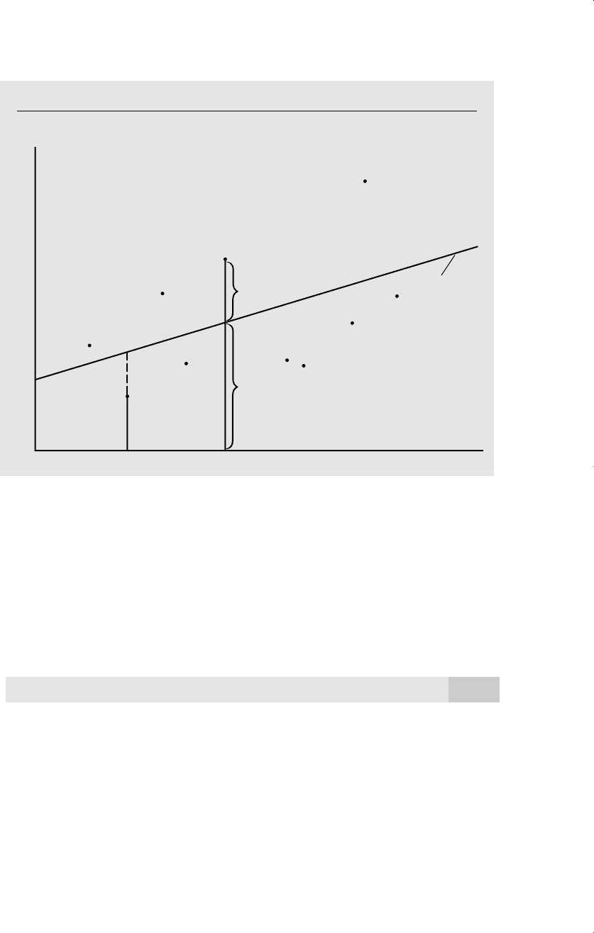
Figure 2.4

Fitted values and residuals.

y  

 

 Fitted value

 residual

d 7/14/99 4:30 PM Page 31

obtained for a given sample of data, a new sample will generate a different slope and

intercept in equation (2.23).

In most cases the slope estimate, which we can write as



yˆ/x, (2.24)

is of primary interest. It tells us the amount by which yˆ changes when x increases by

one unit. Equivalently,

yˆ 



x, (2.25)

so that given any change in x (whether positive or negative), we can compute the pre-

dicted change in y.

We now present several examples of simple regression obtained by using real data.

In other words, we find the intercept and slope estimates with equations (2.17) and

(2.19). Since these examples involve many observations, the calculations were done

using an econometric software package. At this point, you should be careful not to read

too much into these regressions; they are not necessarily uncovering a causal relation-

ship. We have said nothing so far about the statistical properties of OLS. In Section 2.5,

we consider statistical properties after we explicitly impose assumptions on the popu-

lation model equation (2.1).

EXAMPLE 2.3

(CEO Salary and Return on Equity)

For the population of chief executive officers, let y be annual salary (salary) in thousands of

dollars. Thus, y  856.3 indicates an annual salary of $856,300, and y  1452.6 indicates

a salary of $1,452,600. Let x be the average return equity (roe) for the CEO’s firm for the

previous three years. (Return on equity is defined in terms of net income as a percentage

of common equity.) For example, if roe  10, then average return on equity is 10 percent.

To study the relationship between this measure of firm performance and CEO com-

pensation, we postulate the simple model

salary 







roe  u.

The slope parameter



measures the change in annual salary, in thousands of dollars, when

return on equity increases by one percentage point. Because a higher roe is good for the

company, we think



 0.

The data set CEOSAL1.RAW contains information on 209 CEOs for the year 1990; these

data were obtained from Business Week (5/6/91). In this sample, the average annual salary

is $1,281,120, with the smallest and largest being $223,000 and $14,822,000, respective-

ly. The average return on equity for the years 1988, 1989, and 1990 is 17.18 percent, with

the smallest and largest values being 0.5 and 56.3 percent, respectively.

Using the data in CEOSAL1.RAW, the OLS regression line relating salary to roe is

sal

ary  963.191  18.501 roe, (2.26)

Part 1 Regression Analysis with Cross-Sectional Data

d 7/14/99 4:30 PM Page 32

where the intercept and slope estimates have been rounded to three decimal places; we

use “salary hat” to indicate that this is an estimated equation. How do we interpret the

equation? First, if the return on equity is zero, roe  0, then the predicted salary is the inter-

cept, 963.191, which equals $963,191 since salary is measured in thousands. Next, we can

write the predicted change in salary as a function of the change in roe: sal

ary  18.501

(roe). This means that if the return on equity increases by one percentage point, roe 

1, then salary is predicted to change by about 18.5, or $18,500. Because (2.26) is a linear

equation, this is the estimated change regardless of the initial salary.

We can easily use (2.26) to compare predicted salaries at different values of roe.

Suppose roe  30. Then sal

ary  963.191  18.501(30)  1518.221, which is just over

$1.5 million. However, this does not mean that a particular CEO whose firm had an

roe  30 earns $1,518,221. There are many other factors that affect salary. This is just

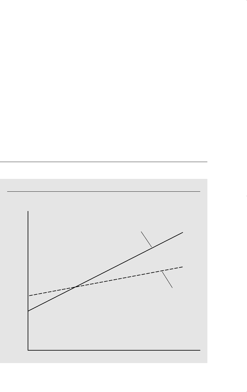
our prediction from the OLS regression line (2.26). The estimated line is graphed in Fig-

ure 2.5, along with the population regression function E(salary兩roe). We will never know

the PRF, so we cannot tell how close the SRF is to the PRF. Another sample of data will

give a different regression line, which may or may not be closer to the population regres-

sion line.

Chapter 2 The Simple Regression Model

Figure 2.5

The OLS regression line sa

lary  963.191  18.50 roe and the (unknown) population

regression function.

salary

963.191

salary  963.191  18.501 roe

E(salaryroe)  

 

roe

d 7/14/99 4:30 PM Page 33

EXAMPLE 2.4

(Wage and Education)

For the population of people in the work force in 1976, let y  wage, where wage is mea-

sured in dollars per hour. Thus, for a particular person, if wage  6.75, the hourly wage is

$6.75. Let x  educ denote years of schooling; for example, educ  12 corresponds to a

complete high school education. Since the average wage in the sample is $5.90, the con-

sumer price index indicates that this amount is equivalent to $16.64 in 1997 dollars.

Using the data in WAGE1.RAW where n  526 individuals, we obtain the following OLS

regression line (or sample regression function):

waˆge 0.90  0.54 educ. (2.27)

We must interpret this equation with caution. The intercept of 0.90 literally means that a

person with no education has a predicted hourly wage of 90 cents an hour. This, of

course, is silly. It turns out that no one in the sample has less than eight years of education,

which helps to explain the crazy prediction for a zero education value. For a person with

eight years of education, the predicted wage

is waˆge 0.90  0.54(8)  3.42, or

$3.42 per hour (in 1976 dollars).

The slope estimate in (2.27) implies that

one more year of education increases hourly

wage by 54 cents an hour. Therefore, four

more years of education increase the pre-

dicted wage by 4(0.54)  2.16 or $2.16 per hour. These are fairly large effects. Because of

the linear nature of (2.27), another year of education increases the wage by the same

amount, regardless of the initial level of education. In Section 2.4, we discuss some meth-

ods that allow for nonconstant marginal effects of our explanatory variables.

EXAMPLE 2.5

(Voting Outcomes and Campaign Expenditures)

The file VOTE1.RAW contains data on election outcomes and campaign expenditures for

173 two-party races for the U.S. House of Representatives in 1988. There are two candi-

dates in each race, A and B. Let voteA be the percentage of the vote received by Candidate

A and shareA be the the percentage of total campaign expenditures accounted for by

Candidate A. Many factors other than shareA affect the election outcome (including the

quality of the candidates and possibly the dollar amounts spent by A and B). Nevertheless,

we can estimate a simple regression model to find out whether spending more relative to

one’s challenger implies a higher percentage of the vote.

The estimated equation using the 173 observations is

vot

eA  40.90  0.306 shareA. (2.28)

This means that, if the share of Candidate A’s expenditures increases by one percent-

age point, Candidate A receives almost one-third of a percentage point more of the

Part 1 Regression Analysis with Cross-Sectional Data

QUESTION 2.2

The estimated wage from (2.27), when educ  8, is $3.42 in 1976

dollars. What is this value in 1997 dollars? (Hint: You have enough

information in Example 2.4 to answer this question.)

d 7/14/99 4:30 PM Page 34

total vote. Whether or not this is a causal effect is unclear, but the result is what we

might expect.

In some cases, regression analysis is not used to determine causality but to simply

look at whether two variables are positively or negatively related, much like a standard

correlation analysis. An example of this

occurs in Problem 2.12, where you are

asked to use data from Biddle and

Hamermesh (1990) on time spent sleeping

and working to investigate the tradeoff

between these two factors.

A Note on Terminolgy

In most cases, we will indicate the estimation of a relationship through OLS by writing

an equation such as (2.26), (2.27), or (2.28). Sometimes, for the sake of brevity, it is

useful to indicate that an OLS regression has been run without actually writing out the

equation. We will often indicate that equation (2.23) has been obtained by OLS in say-

ing that we run the regression of

y on x, (2.29)

or simply that we regress y on x. The positions of y and x in (2.29) indicate which is the

dependent variable and which is the independent variable: we always regress the depen-

dent variable on the independent variable. For specific applications, we replace y and x

with their names. Thus, to obtain (2.26), we regress salary on roe or to obtain (2.28),

we regress voteA on shareA.

When we use such terminology in (2.29), we will always mean that we plan to esti-

mate the intercept,



, along with the slope,



. This case is appropriate for the vast

majority of applications. Occasionally, we may want to estimate the relationship

between y and x assuming that the intercept is zero (so that x  0 implies that yˆ  0);

we cover this case briefly in Section 2.6. Unless explicitly stated otherwise, we always

estimate an intercept along with a slope.

2.3 MECHANICS OF OLS

In this section, we cover some algebraic properties of the fitted OLS regression line.

Perhaps the best way to think about these properties is to realize that they are features

of OLS for a particular sample of data. They can be contrasted with the statistical prop-

erties of OLS, which requires deriving features of the sampling distributions of the esti-

mators. We will discuss statistical properties in Section 2.5.

Several of the algebraic properties we are going to derive will appear mundane.

Nevertheless, having a grasp of these properties helps us to figure out what happens to

the OLS estimates and related statistics when the data are manipulated in certain ways,

such as when the measurement units of the dependent and independent variables change.

Chapter 2 The Simple Regression Model

QUESTION 2.3

In Example 2.5, what is the predicted vote for Candidate A if shareA

 60 (which means 60 percent)? Does this answer seem reasonable?

d 7/14/99 4:30 PM Page 35

Fitted Values and Residuals

We assume that the intercept and slope estimates,



and



, have been obtained for the

given sample of data. Given



and



, we can obtain the fitted value yˆ

for each obser-

vation. [This is given by equation (2.20).] By definition, each fitted value of yˆ

is on the

OLS regression line. The OLS residual associated with observation i, uˆ

, is the differ-

ence between y

and its fitted value, as given in equation (2.21). If uˆ

is positive, the line

underpredicts y

; if uˆ

is negative, the line overpredicts y

. The ideal case for observation

i is when uˆ

 0, but in most cases every residual is not equal to zero. In other words,

none of the data points must actually lie on the OLS line.

EXAMPLE 2.6

(CEO Salary and Return on Equity)

Table 2.2 contains a listing of the first 15 observations in the CEO data set, along with the

fitted values, called salaryhat, and the residuals, called uhat.

Table 2.2

Fitted Values and Residuals for the First 15 CEOs

obsno roe salary salaryhat uhat

1 14.1 1095 1224.058 129.0581

2 10.9 1001 1164.854 163.8542

3 23.5 1122 1397.969 275.9692

4 5.9 578 1072.348 494.3484

5 13.8 1368 1218.508 149.4923

6 20.0 1145 1333.215 188.2151

7 16.4 1078 1266.611 188.6108

8 16.3 1094 1264.761 170.7606

9 10.5 1237 1157.454 79.54626

10 26.3 833 1449.773 616.7726

11 25.9 567 1442.372 875.3721

12 26.8 933 1459.023 526.0231

Part 1 Regression Analysis with Cross-Sectional Data

continued

d 7/14/99 4:30 PM Page 36

Table 2.2 (

concluded

)

obsno roe salary salaryhat uhat

13 14.8 1339 1237.009 101.9911

14 22.3 937 1375.768 438.7678

15 56.3 2011 2004.808 006.191895

The first four CEOs have lower salaries than what we predicted from the OLS regression line

(2.26); in other words, given only the firm’s roe, these CEOs make less than what we pre-

dicted. As can be seen from the positive uhat, the fifth CEO makes more than predicted

from the OLS regression line.

Algebraic Properties of OLS Statistics

There are several useful algebraic properties of OLS estimates and their associated sta-

tistics. We now cover the three most important of these.

(1) The sum, and therefore the sample average of the OLS residuals, is zero.

Mathematically,

兺

i1

uˆ

 0.

(2.30)

This property needs no proof; it follows immediately from the OLS first order condi-

tion (2.14), when we remember that the residuals are defined by uˆ

 y









In other words, the OLS estimates



and



are chosen to make the residuals add up to

zero (for any data set). This says nothing about the residual for any particular observa-

tion i.

(2) The sample covariance between the regressors and the OLS residuals is zero.

This follows from the first order condition (2.15), which can be written in terms of the

residuals as

兺

i1

uˆ

 0.

(2.31)

The sample average of the OLS residuals is zero, so the left hand side of (2.31) is pro-

portional to the sample covariance between x

and uˆ

(3) The point (x¯,y¯) is always on the OLS regression line. In other words, if we take

equation (2.23) and plug in x¯ for x, then the predicted value is y¯. This is exactly what

equation (2.16) shows us.

Chapter 2 The Simple Regression Model

d 7/14/99 4:30 PM Page 37

EXAMPLE 2.7

(Wage and Education)

For the data in WAGE1.RAW, the average hourly wage in the sample is 5.90, rounded to

two decimal places, and the average education is 12.56. If we plug educ  12.56 into the

OLS regression line (2.27), we get waˆge 0.90  0.54(12.56)  5.8824, which equals

5.9 when rounded to the first decimal place. The reason these figures do not exactly agree

is that we have rounded the average wage and education, as well as the intercept and slope

estimates. If we did not initially round any of the values, we would get the answers to agree

more closely, but this practice has little useful effect.

Writing each y

as its fitted value, plus its residual, provides another way to intepret

an OLS regression. For each i, write

 yˆ

 uˆ

. (2.32)

From property (1) above, the average of the residuals is zero; equivalently, the sample

average of the fitted values, yˆ

, is the same as the sample average of the y

, or yˆ

 y¯.

Further, properties (1) and (2) can be used to show that the sample covariance

between yˆ

and uˆ

is zero. Thus, we can view OLS as decomposing each y

into two

parts, a fitted value and a residual. The fitted values and residuals are uncorrelated in

the sample.

Define the total sum of squares (SST), the explained sum of squares (SSE), and

the residual sum of squares (SSR) (also known as the sum of squared residuals), as

follows:

SST ⬅

兺

i1

 y¯)

(2.33)

SSE ⬅

兺

i1

(yˆ

 y¯)

(2.34)

SSR ⬅

兺

i1

uˆ

(2.35)

SST is a measure of the total sample variation in the y

; that is, it measures how spread

out the y

are in the sample. If we divide SST by n



1, we obtain the sample variance

of y, as discussed in Appendix C. Similarly, SSE measures the sample variation in the

yˆ

(where we use the fact that yˆ

 y¯), and SSR measures the sample variation in the uˆ

The total variation in y can always be expressed as the sum of the explained variation

and the unexplained variation SSR. Thus,

SST  SSE  SSR. (2.36)

Part 1 Regression Analysis with Cross-Sectional Data

d 7/14/99 4:30 PM Page 38

Proving (2.36) is not difficult, but it requires us to use all of the properties of the sum-

mation operator covered in Appendix A. Write

兺

i1

 y¯)



兺

i1

[(y

 yˆ

)  (yˆ

 y¯)]



兺

i1

[uˆ

 (yˆ

 y¯)]



兺

i1

uˆ

 2

兺

i1

uˆ

(yˆ

 y¯) 

兺

i1

(yˆ

 y¯)

 SSR  2

兺

i1

uˆ

(yˆ

 y¯)  SSE.

Now (2.36) holds if we show that

兺

i1

uˆ

(yˆ

 y¯)  0.

(2.37)

But we have already claimed that the sample covariance between the residuals and the

fitted values is zero, and this covariance is just (2.37) divided by n1. Thus, we have

established (2.36).

Some words of caution about SST, SSE, and SSR are in order. There is no uniform

agreement on the names or abbreviations for the three quantities defined in equations

(2.33), (2.34), and (2.35). The total sum of squares is called either SST or TSS, so there

is little confusion here. Unfortunately, the explained sum of squares is sometimes called

the “regression sum of squares.” If this term is given its natural abbreviation, it can eas-

ily be confused with the term residual sum of squares. Some regression packages refer

to the explained sum of squares as the “model sum of squares.”

To make matters even worse, the residual sum of squares is often called the “error

sum of squares.” This is especially unfortunate because, as we will see in Section 2.5,

the errors and the residuals are different quantities. Thus, we will always call (2.35) the

residual sum of squares or the sum of squared residuals. We prefer to use the abbrevia-

tion SSR to denote the sum of squared residuals, because it is more common in econo-

metric packages.

Goodness-of-Fit

So far, we have no way of measuring how well the explanatory or independent variable,

x, explains the dependent variable, y. It is often useful to compute a number that sum-

marizes how well the OLS regression line fits the data. In the following discussion, be

sure to remember that we assume that an intercept is estimated along with the slope.

Assuming that the total sum of squares, SST, is not equal to zero—which is true

except in the very unlikely event that all the y

equal the same value—we can divide

(2.36) by SST to get 1  SSE/SST  SSR/SST. The R-squared of the regression,

sometimes called the coefficient of determination, is defined as

Chapter 2 The Simple Regression Model

d 7/14/99 4:30 PM Page 39

 SSE/SST  1  SSR/SST. (2.38)

is the ratio of the explained variation compared to the total variation, and thus it is

interpreted as the fraction of the sample variation in y that is explained by x. The sec-

ond equality in (2.38) provides another way for computing R

From (2.36), the value of R

is always between zero and one, since SSE can be no

greater than SST. When interpreting R

, we usually multiply it by 100 to change it into

a percent: 100R

is the percentage of the sample variation in y that is explained by x.

If the data points all lie on the same line, OLS provides a perfect fit to the data. In

this case, R

 1. A value of R

that is nearly equal to zero indicates a poor fit of the

OLS line: very little of the variation in the y

is captured by the variation in the yˆ

(which

all lie on the OLS regression line). In fact, it can be shown that R

is equal to the square

of the sample correlation coefficient between y

and yˆ

. This is where the term

“R-squared” came from. (The letter R was traditionally used to denote an estimate of a

population correlation coefficient, and its usage has survived in regression analysis.)

EXAMPLE 2.8

(CEO Salary and Return on Equity)

In the CEO salary regression, we obtain the following:

sal

ary  963.191  18.501 roe (2.39)

n  209, R

 0.0132

We have reproduced the OLS regression line and the number of observations for clarity.

Using the R-squared (rounded to four decimal places) reported for this equation, we can

see how much of the variation in salary is actually explained by the return on equity. The

answer is: not much. The firm’s return on equity explains only about 1.3% of the variation

in salaries for this sample of 209 CEOs. That means that 98.7% of the salary variations for

these CEOs is left unexplained! This lack of explanatory power may not be too surprising

since there are many other characteristics of both the firm and the individual CEO that

should influence salary; these factors are necessarily included in the errors in a simple

regression analysis.

In the social sciences, low R-squareds in regression equations are not uncommon,

especially for cross-sectional analysis. We will discuss this issue more generally under

multiple regression analysis, but it is worth emphasizing now that a seemingly low R-

squared does not necessarily mean that an OLS regression equation is useless. It is still

possible that (2.39) is a good estimate of the ceteris paribus relationship between salary

and roe; whether or not this is true does not depend directly on the size of R-squared.

Students who are first learning econometrics tend to put too much weight on the size of

the R-squared in evaluating regression equations. For now, be aware that using

R-squared as the main gauge of success for an econometric analysis can lead to trouble.

Sometimes the explanatory variable explains a substantial part of the sample varia-

tion in the dependent variable.

Part 1 Regression Analysis with Cross-Sectional Data

d 7/14/99 4:30 PM Page 40

Wooldridge - Introductory Econometrics - A Modern Approach, 2e

Подождите немного. Документ загружается.