Warren J., Weimer H. Subdivision Methods for Geometric Design. A Constructive Approach
Подождите немного. Документ загружается.

174 CHAPTER 6 Variational Schemes for Bounded Domains
form of the problem. In the following section, we will show that solutions to this
new equation minimize the original variational functional.
Assuming that the matrix
E
k
is the correct analog of the difference mask d
k
[x],
we are left with deriving the correct matrix analog of
d
0
[x
2
k
]. Note that the ef-
fect of replacing
x by x
2
in a generating function (i.e., substituting p[x] → p[x
2
])is
to spread the coefficients of the generating function and to insert zeros between
them (i.e., upsample the vector
p). In matrix terms, upsampling the vector p from
the coarse grid
1
2
k−1
Z onto the fine grid
1
2
k
Z can be modeled via multiplication
by the upsampling matrix
U
k−1
whose ijth entry is 1 if i == 2j and 0 otherwise.
(Note that the
ith row of U
k−1
is indexed by the grid point
i
2
k
∈ and the jth
column of
U
k−1
is indexed by the grid point
j
2
k−1
∈ .) Based on this observation,
the matrix analog of
d
0
[x
2
] is U
0
E
0
. More generally, the matrix analog of d
0
[x
2
k
] is the
product of
E
0
multiplied by a sequence of upsampling matrices U
0
, U
1
, ..., U
k−1
.
Consequently, the variational matrix analog of equation 6.15 is
E
k
p
k
== U
k−1
···U
0
E
0
p
0
. (6.16)
(Note that the extra power of
2
k
in equation 6.15 is absorbed into the matrix
E
k
as
a constant of integration for the grid
1
2
k
Z.)
Equation 6.16 relates a vector
p
k
defined on the fine grid
1
2
k
Z, with the vector
p
0
defined on the coarse grid Z. As in the differential case, our goal is to construct
a sequence of subdivision matrices
S
k−1
that relates successive solutions to equa-
tion 6.16. These subdivision matrices
S
k−1
satisfy the following relation involving
the inner product matrices
E
k−1
and E
k
at successive scales.
THEOREM
6.3
For all k > 0, let S
k
be a sequence of matrices satisfying the two-scale
relation
E
k
S
k−1
== U
k−1
E
k−1
. (6.17)
If the vectors p
k
satisfy the subdivision relation p
k
= S
k−1
p
k−1
for all k > 0,
then
p
k
and p
0
satisfy the multiscale relation of equation 6.16.
Proof The proof proceeds by induction. For k = 1, the theorem follows trivially.
More generally, assume that
E
k−1
p
k−1
== U
k−2
···U
0
E
0
p
0
holds by the in-
ductive hypothesis. Multiplying both sides of this equation by
U
k−1
and
replacing
U
k−1
E
k−1
by E
k
S
k−1
on the left-hand side yields the desired result.
6.2 Subdivision for Natural Cubic Splines 175
A subdivision scheme satisfying equation 6.17 requires a certain commutativity
relationship to hold among the inner product matrices, subdivision matrices, and
upsampling matrices. This relation has an interesting interpretation in terms of the
Euler-Lagrange theorem. Recall that given a variational functional
E this theorem
constructs a partial differential equation whose solutions are extremal functions
for
E. The discrete version of the variational functional
E[p] on the grid
1
2
k
Z is the
expression
p
T
k
E
k
p
k
, where E
k
is the inner product matrix associated with E. Now,
observe that this quadratic function in the entries of the vector
p
k
is minimized by
exactly those vectors
p
k
satisfying E
k
p
k
== 0. In other words, the linear equation
E
k
p
k
== 0 can be viewed as the discretized version of the partial differential equation
corresponding to
E.
If the products
E
k−1
p
k−1
and E
k
p
k
are viewed as taking discrete differences of
the vectors
p
k−1
and p
k
corresponding to this partial difference equation, equa-
tion 6.17 states that differencing the vector
p
k−1
over the coarse grid
1
2
k−1
Z and
then upsampling those differences to the next finer grid
1
2
k
Z should be the same as
subdividing the vector
p
k−1
using the subdivision matrix S
k−1
and then differencing
those coefficients with respect to the finer grid
1
2
k
Z using the matrix E
k
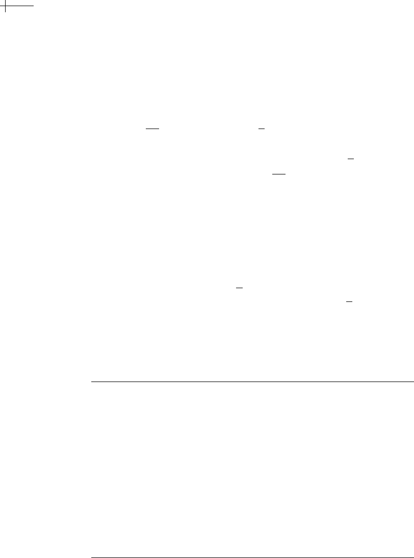
. Figure 6.3
illustrates this commutativity constraint in a diagram, stating that the two paths
from the upper left to the lower right should yield the same result (i.e., the same
differences over the fine grid
1
2
k
Z).
The effect of several rounds of subdivision with these matrices
S
k
is to define a
sequence of vectors
p
k
whose differences E
k
p
k
replicate the differences E
0
p
0
on Z
and are zero on the remaining grid points in
1
2
k
Z. As a result, the limiting function
p
k1
S
k1
p
k1
E
k1
p
k1
E
k
S
k1
p
k1
U
k
E
k1
p
k1
Difference
Upsample
Subdivide
Difference
Figure 6.3 The two-scale relation requires commutativity between inner products, upsampling, and
subdivision.
176 CHAPTER 6 Variational Schemes for Bounded Domains
123
4
15
10
5
5
10
15
1 2 3
4
15
10
5
5
10
15
1 2 3
4
15
10
5
5
10
15
1 2 3
4
15
10
5
5
10
15
1 2 3
4
2
3
4
5
1 2 3
4
1.5
2
2.5
3
3.5
4
4.5
1 2 3
4
1.5
2
2.5
3
3.5
4
4.5
1 2 3
4
1.5
2
2.5
3
3.5
4
4.5
(a)
(b)
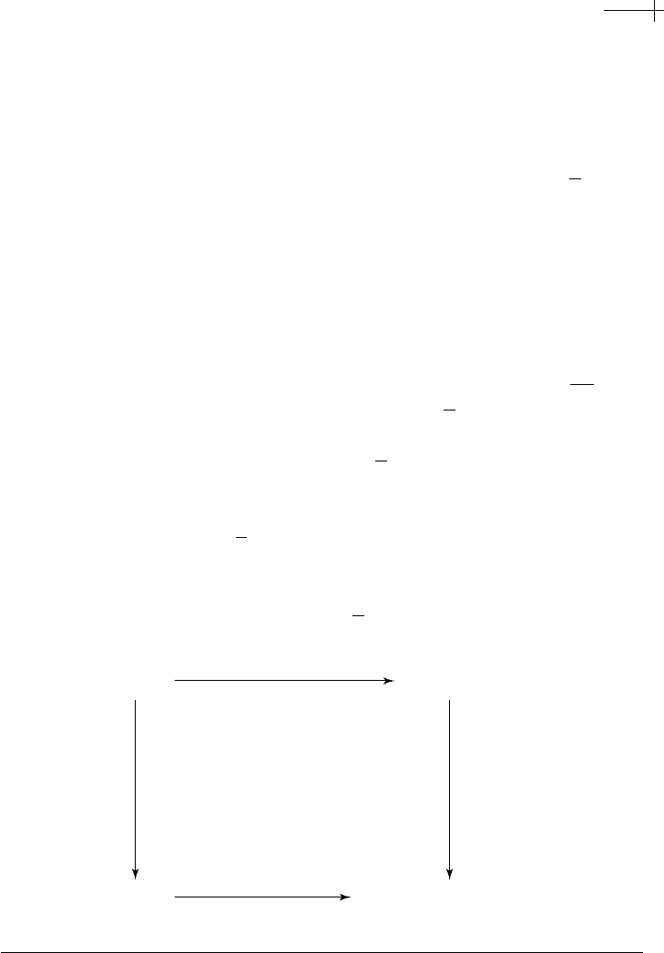
Figure 6.4 A sequence of polygons p
k
defined by natural cubic subdivision (a) and plots of the differences
E
k
p
k
(b).
p
∞
[x] satisfies the partial differential equation associated with the variational func-
tional everywhere except on the grid
Z. Figure 6.4 illustrates the behavior of these
differences using the subdivision rules for natural cubic splines derived in the next
section. The top row of plots shows the effects of three rounds of subdivision. The
bottom row of plots shows the differences
E
k
p
k
for k == 0...3.
6.2.4 Subdivision Rules for Natural Cubic Splines
Given equation 6.17, our approach is to use this relation in computing the subdivi-
sion matrix
S
k−1
. In the next section, we show that the limit functions produced by
the resulting scheme are minimizers of the variational functional
E[p]. We proceed
by noting that equation 6.17 does not uniquely determine the subdivision matrix
S
k−1
, because the inner product matrix E
k
has a non-empty null space and thus
is not invertible. For the inner product of equation 6.11, the differences
E
k
p
k
are
zero when
p
k
is the constant vector or the linearly varying vector p
k
[[ i ]] = i . This
observation is consistent with the fact that the continuous variational functional
E yields zero energy for linear functions. Instead of attempting to invert E
k
,we
focus on computing a simple sequence of subdivision matrices
S
k−1
that satisfies
equation 6.17 and defines a convergent subdivision scheme.
6.2 Subdivision for Natural Cubic Splines 177
As done in computing the inner product matrices, our approach is first to
compute the stationary subdivision matrix
S for the domain = [0, ∞]. This matrix
encodes the subdivision rules for the endpoint of a natural cubic spline and can be
used to construct the subdivision matrices
S
k−1
for any other finite intervals. The
main advantage of choosing this domain is that due to the inner product matrices
E
k
satisfying E
k
== 8
k
E equation 6.17 reduces to a stationary equation of the form
8E S == UE. The factor of 8 in this equation arises from integrating the product
of second derivatives. If we assume the subdivision matrix
S to be a uniform two-
slanted matrix sufficiently far from the endpoint of
x == 0, the equation 8E S == UE
has the matrix form
8
⎛
⎜
⎜
⎜
⎜
⎜
⎜
⎝
1 −210000.
−25−41000.
1 −46−4100.
01−46−410.
001−46−41.
........
⎞
⎟
⎟
⎟
⎟
⎟
⎟
⎠
⎛
⎜
⎜
⎜
⎜
⎜
⎜
⎜
⎜
⎜
⎜
⎜
⎝
s[−4] s[−3] 0 .
s[−2] s[−1] 0 .
s[2] s[0] s[2] .
0 s[1] s[1] .
0 s[2] s[0] .
0 0 s[1] .
0 0 s[2] .
....
⎞
⎟
⎟
⎟
⎟
⎟
⎟
⎟
⎟
⎟
⎟
⎟
⎠
==
⎛
⎜
⎜
⎜
⎜
⎜
⎜
⎝
100.
000.
010.
000.
001.
....
⎞
⎟
⎟
⎟
⎟
⎟
⎟
⎠
⎛
⎜
⎜
⎝
1 −21.
−25−4 .
1 −46.
....
⎞
⎟
⎟
⎠
.
The unknowns
s[i] with negative index encapsulate the boundary behavior of S,
whereas the unknowns
s[i] with non-negative index encapsulate the uniform sub-
division rules for cubic B-splines. Solving for these unknowns yields a subdivision
matrix
S for the domain = [0, ∞] of the form
S =
⎛
⎜
⎜
⎜
⎜
⎜
⎜
⎜
⎜
⎜
⎜
⎜
⎜
⎝
100.
1
2
1
2
0 .
1
8
3
4
1
8
.
0
1
2
1
2
.
0
1
8
3
4
.
00
1
2
.
....
⎞
⎟
⎟
⎟
⎟
⎟
⎟
⎟
⎟
⎟
⎟
⎟
⎟
⎠
.

178 CHAPTER 6 Variational Schemes for Bounded Domains
Note that the interior rows of S agree with the subdivision rules for uniform
cubic B-splines with the subdivision rule at the endpoint forcing interpolation. In
fact, the subdivision matrices
S
k
for an arbitrary interval with integer endpoints
have the same structure: the first and last row in the matrix are standard unit vectors,
and all remaining rows are shifts of the fundamental sequences
{
1
2
,
1
2
} and {
1
8
,
3
4
,
1
8
}.
The behavior of the scheme at the endpoints of this interval can be analyzed by
constructing the explicit piecewise cubic representation for
N [x].If = [0, 4], the
five basis functions comprising
N [x] can be written in piecewise cubic B
´
ezier form
as follows:
0
1
3
2
3
1
4
3
5
3
2
7
3
8
3
3
10
3
11
3
4
1
2
3
1
3
1
6
000000 0 0 0
0
1
3
2
3
2
3
2
3
1
3
1
6
000 0 0 0
000
1
6
1
3
2
3
2
3
2
3
1
3
1
6
000
000000
1
6
1
3
2
3
2
3
2
3
1
3
0
000000000
1
6
1
3
2
3
1 .
The first row consists of the x coordinates for the control points of the four B
´
ezier
segments as
x varies from 0 to 4. The last five rows are the corresponding B
´
ezier
coefficients of the five basis functions, each row consisting of four consecutive cubic
B
´
ezier functions. The reader can verify that these basis functions are consistent
with the subdivision rules given previously. Note that the middle basis function
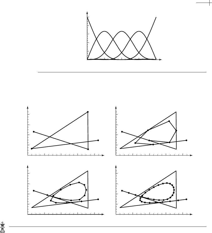
is the uniform cubic basis function. A plot of these basis functions is shown in
Figure 6.5.
This representation confirms that the basis functions are
C
2
piecewise cubics
and satisfy the natural boundary conditions (i.e., their second derivatives at
0 and
4 are zero). Given the subdivision matrices S
k
and an initial set of coefficients
p
0
, the scheme can be used to define increasingly dense sets of coefficients p
k
via
the relation
p
k
= S
k−1
p
k−1
. If we interpolate the coefficients of p
k
with the piecewise
linear function
p
k
[x] satisfying p
k
[
i
2
k
] = p
k
[[ i ]] , the functions p
k
[x] uniformly converge
to a piecewise cubic function
p
∞
[x] ∈ C
2
. (See [157] for a matrix version of the
convergence analysis of Chapter 3.)
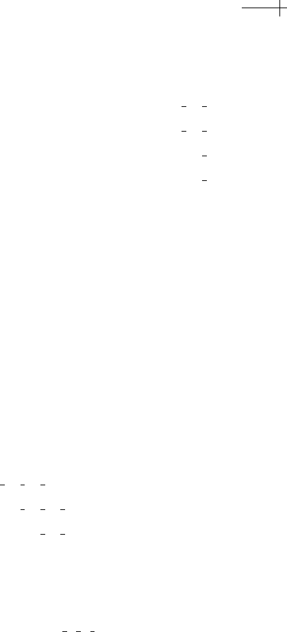
Given an initial set of coefficients
p
0
, applying the subdivision scheme yields
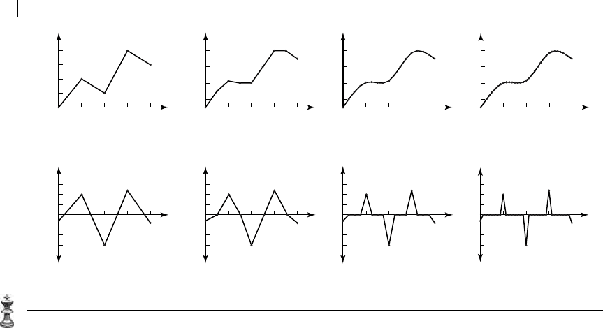
increasingly dense approximations of the natural cubic spline. Figure 6.6 shows
three rounds of this subdivision procedure applied to the initial coefficients
p
0
6.2 Subdivision for Natural Cubic Splines 179
1
2
3
4
.2
.4
.6
.8
1
Figure 6.5 Plots of the five basis functions comprising the basis vector N
0
[x] for the domain
= [0, 4].
.2 .4 .6
.8
.2
.4
.6
.8
.2 .4 .6
.8
.2
.4
.6
.8
.2 .4 .6
.8
.2
.4
.6
.8
.2 .4 .6
.8
.2
.4
.6
.8
Figure 6.6 Progression of the natural cubic spline subdivision process starting from the initial control polygon
(upper left).

180 CHAPTER 6 Variational Schemes for Bounded Domains
(upper left). Note that here the scheme is applied parametrically; that is, the control
points are points in two dimensions, and subdivision is applied to both coordinates
to obtain the next denser shape.
6.3 Minimization of the Variational Scheme
The previous section constructed a relation of the form E
k
S
k−1
== U
k−1
E
k−1
that
models the finite difference relation
d
k
[x] s
k−1
[x] == 2d
k−1
[x
2
] arising from the dif-
ferential method. However, we offered no formal proof that subdivision schemes
constructed using the differential method converged to solutions to the differen-
tial equation. Instead, we simply analyzed the convergence and smoothness of
the resulting schemes. In this section, we show that subdivision matrices satisfying
equation 6.17 define a subdivision scheme whose limit functions
p
∞
[x] are minimiz-
ers of
E[p] in the following sense: over the space of all functions (with well-defined
energy) interpolating a fixed set of values on
∩Z, the limit function p
∞
[x] produced
by this subdivision scheme has minimal energy.
Our approach in proving this minimization involves three steps. First, we con-
sider the problem of enforcing interpolation for natural cubic splines using interpo-
lation matrices. Next, we show that these interpolation matrices can also be used
to compute the exact value of the variational functional
E[p
∞
]. Finally, we set up a
multiresolution framework based on the inner product associated with
E and prove
that
p
∞
[x] is a minimizer of E in this framework.
6.3.1 Interpolation with Natural Cubic Splines
Due to the linearity of the subdivision process, any limit function p
∞
[x] can be
written as the product of the row vector of basis functions
N
0
[x] associated with
the subdivision scheme and a column vector
p
0
; that is, p
∞
[x] = N
0
[x]p
0
. Remember
that
N
0
[x] represents the vector of basis functions associated with the variational
subdivision scheme;
N
0
[x] is the finite element basis used in constructing the inner
product matrix
E
0
. Due to the convergence of the subdivision scheme for natural
cubic splines, the continuous basis
N
0
[x] can be evaluated on the grid Z (restricted
to
) to form the interpolation matrix N
0
.
In the stationary case where
= [0, ∞], all of the interpolation matrices N
k
agree
with a single interpolation matrix
N that satisfies the recurrence of equation 6.2
(i.e.,
U
T
NS == N). This matrix N is tridiagonal because the natural cubic spline basis
functions are supported over four consecutive intervals. If the non-zero entries
6.3 Minimization of the Variational Scheme 181
of N are treated as unknowns, for natural cubic splines this recurrence has the
matrix form
⎛
⎜
⎜
⎝
10000.
00100.
00001.
......
⎞
⎟
⎟
⎠
⎛
⎜
⎜
⎜
⎜
⎜
⎜
⎜
⎜
⎜
⎜
⎝
n[−2] n[−1]000.
n[1] n[0] n[1] 0 0 .
0 n[1] n[0] n[1] 0 .
0 0 n[1] n[0] n[1] .
0 0 0 n[1] n[0] .
. . ....
⎞
⎟
⎟
⎟
⎟
⎟
⎟
⎟
⎟
⎟
⎟
⎠
⎛
⎜
⎜
⎜
⎜
⎜
⎜
⎜
⎜
⎜
⎜
⎝
10.
1
2
1
2
.
1
8
3
4
.
0
1
2
.
0
1
8
.
...
⎞
⎟
⎟
⎟
⎟
⎟
⎟
⎟
⎟
⎟
⎟
⎠
==
⎛
⎜
⎜
⎜
⎜
⎝
n[−2] n[−1] .
n[1] n[0] .
0 n[1] .
...
⎞
⎟
⎟
⎟
⎟
⎠
.
Again, the unknowns n[ i ] with negative index encapsulate the boundary behavior
of the natural cubic splines, whereas the unknowns
n[ i ] with non-negative index
encapsulate the interpolation mask for cubic B-splines. After further constraining
the rows of the interpolation matrix
N to sum to one, there exists a unique solution
for the interpolation matrix
N of the form
N =
⎛
⎜
⎜
⎜
⎜
⎜
⎜
⎜
⎜
⎝
1000.
1
6
2
3
1
6
0 .
0
1
6
2
3
1
6
.
00
1
6
2
3
.
.....
⎞
⎟
⎟
⎟
⎟
⎟
⎟
⎟
⎟
⎠
.
More generally, if is an arbitrary finite interval with endpoints in Z, then N
0
is a
tridiagonal matrix whose first and last rows are of the form
{1, 0, ...} and {..., 0, 1},
and whose interior rows have the form
{..., 0,
1
6
,
2
3
,
1
6
, 0, ...}.
The interpolation matrices play several vital roles in manipulating natural cubic
splines. First, the interpolation matrix gives us a systematic method of handling
the interpolation conditions associated with the original spline problem. Given a
natural cubic spline of the form
p
∞
[x] = N
0
[x]p
0
, the values of p
∞
[x] on Z are exactly
N
0
p
0
. Thus, p
∞
[x] interpolates the values N
0
p
0
on the grid Z. To interpolate an
arbitrary collection of values
b, the initial coefficients p
0
must be chosen so as
182 CHAPTER 6 Variational Schemes for Bounded Domains
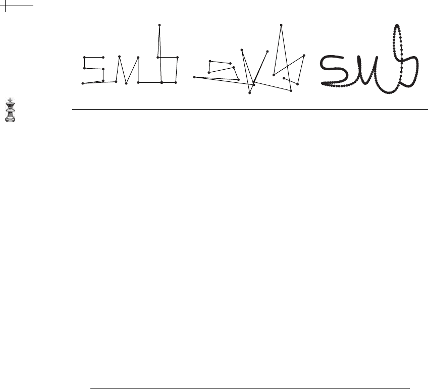
Figure 6.7 Using the inverse of the interpolation matrix to force interpolation of the vertices of a control
polygon.
to satisfy p
0
= (N
0
)
−1
b. For example, if the vertices of the curve in the left-hand
image of Figure 6.7 are denoted by
b, the center image of Figure 6.7 depicts the
control polygon
p
0
= (N
0
)
−1
b. The right-hand image of the figure shows the result
of applying four rounds of natural cubic spline subdivision to
p
0
, converging to a
curve that interpolates the original points
b.
6.3.2 Exact Inner Products for the Variational Scheme
Another important application of the interpolation matrices N
k
lies in computing
the inner product of limit functions produced by the subdivision scheme, that is,
functions of the form
p
∞
[x] = N
0
[x]p
0
and q
∞
[x] = N
0
[x]q
0
where N
0
[x] is the vector
of scaling functions associated with the variational scheme. In the previous section,
we constructed the inner product matrices
E
k
with the property that p
∞
, q
∞
is
the limit of
p
T
k
E
k
q
k
as k →∞. Instead of computing this inner product as a limit,
the following theorem expresses the exact value of
p
∞
, q
∞
in terms of a modified
discrete inner product matrix of the form
E
0
N
0
.
THEOREM
6.4
Consider a uniformly convergent subdivision scheme whose subdivision
matrices
S
k−1
satisfy equation 6.17, with the matrices E
k
being defined via
a symmetric inner product taken on a bounded domain
. Given two limit
curves
p
∞
[x] and q
∞
[x] for this scheme of the form N
0
[x]p
0
and N
0
[x]q
0
, the
inner product
p
∞
, q
∞
satisfies
p
∞
, q
∞
== p
T
0
E
0
N
0
q
0
,
where N
0
is the interpolation matrix for the scheme.
Proof Given p
0
and q
0
, let p
k
and q
k
be vectors defined via subdivision. Now, con-
sider the continuous functions
p
k
[x] =
N
k
[x]p
k
and q
k
[x] =
N
k
[x]q
k
defined

6.3 Minimization of the Variational Scheme 183
in terms of the finite element basis
N
k
[x] used in constructing the inner
product matrix
E
k
. Due to the linearity of inner products, p
∞
, q
∞
satisfies
p
∞
, q
∞
== p
k
, q
k
+p
∞
− p
k
, q
k
+p
∞
, q
∞
− q
k
.
Due to the uniform convergence of p
k
[x] to p
∞
[x] on the bounded domain
, the inner product p
∞
− p
k
, q
k
converges to zero as k →∞. Because
a similar observation holds for
p
∞
, q
∞
− q
k
, the inner product p
∞
, q
∞
satisfies
p
∞
, q
∞
= lim
k→∞
p
k
, q
k
== lim
k→∞
p
T
k
E
k
q
k
.
Because the subdivision matrices S
k−1
satisfy equation 6.17, the vectors p
k
satisfy equation 6.16 for all k > 0. Replacing p
T
k
E
k
== (E
k
p
k
)
T
by its equiv-
alent left-hand side,
(U
k−1
···U
0
E
0
p
0
)
T
, yields
lim
k→∞
p
T
k
E
T
k
q
k
== lim
k→∞
p
T
0
E
T
0
U
T
0
··· U
T
k−1
q
k
.
Now, the effect of the product U
T
0
··· U
T
k−1
on the vector q
k
is to down-
sample the entries of
q
k
from the grid
1
2
k
Z to the grid Z. Therefore, as
k →∞, the vector U
T
0
··· U
T
k−1
q
k
converges to the values of the limit func-
tion
q
∞
[x] taken on the integer grid Z. However, these values can be com-
puted directly using the interpolation matrix
N
0
via the expression N
0
q
0
.
Thus, the theorem is proven; that is,
lim
k→∞
p
T
0
E
T
0
U
T
0
···U
T
k−1
q
k
== p
T
0
E
0
N
0
q
0
.
For example, let p
0
be the vector consisting of the first coordinate of the ver-
tices of the center polygon in Figure 6.7. If the subsequent vectors
p
k
are defined
via the subdivision relation
p
k
= S
k−1
p
k−1
for natural cubic splines, the energy of
the quadratic B-spline curves associated with these polygons is a scalar of the form
p
T
k
E
k
p
k
. Evaluating this expression for k = 0, 1, ..., 5 yields the energies 71.3139,
42.2004, 34.922, 33.1025, 32.6476, and 32.5338. These energies are converging to the
energy of the natural cubic spline
p
∞
[x] associated with the initial vector p
0
.
The energy of this limit curve can be computed directly by applying Theorem 6.4;
that is,
E[p
∞
] == p
T
0
E
0
N
0
p
0
= 32.4959.